

Abstract
This study aimed to characterize the neural generators of the steady‐state visual evoked potential (SSVEP) to repetitive, 6 Hz pattern‐reversal stimulation. Multichannel scalp recordings of SSVEPs and dipole modeling techniques were combined with functional magnetic resonance imaging (fMRI) and retinotopic mapping in order to estimate the locations of the cortical sources giving rise to the SSVEP elicited by pattern reversal. The time‐varying SSVEP scalp topography indicated contributions from two major cortical sources, which were localized in the medial occipital and mid‐temporal regions of the contralateral hemisphere. Colocalization of dipole locations with fMRI activation sites indicated that these two major sources of the SSVEP were located in primary visual cortex (V1) and in the motion sensitive (MT/V5) areas, respectively. Minor contributions from mid‐occipital (V3A) and ventral occipital (V4/V8) areas were also considered. Comparison of SSVEP phase information with timing information collected in a previous transient VEP study (Di Russo et al. [2005] Neuroimage 24:874–886) suggested that the sequence of cortical activation is similar for steady‐state and transient stimulation. These results provide a detailed spatiotemporal profile of the cortical origins of the SSVEP, which should enhance its use as an efficient clinical tool for evaluating visual‐cortical dysfunction as well as an investigative probe of the cortical mechanisms of visual‐perceptual processing. Hum. Brain Mapp, 2007. © 2006 Wiley‐Liss, Inc.
INTRODUCTION
When a repetitive or flickering visual stimulus is presented at a rate of around 4 Hz or higher, a continuous sequence of oscillatory potential changes are elicited in the visual cortex, which has been termed the steady‐state visual evoked potential (SSVEP). The SSVEP generally appears in scalp recordings as a near‐sinusoidal waveform at the frequency of the driving stimulus or its harmonics [reviewed in Regan, 1989]. The SSVEP was initially considered to serve as a bridge between studies of animal neurophysiology and human psychophysics [Campbell and Maffei, 1970; Campbell and Robson, 1969], and subsequent studies have shown it to be a sensitive electrophysiological index of a variety of visual‐perceptual functions [reviewed in Di Russo et al., 2002a].
The majority of studies that have investigated cortical evoked activity in humans were confined to the transient responses evoked by individual stimuli. The transient visual evoked potential (VEP) to a pattern‐reversal stimulus includes three major early components: the N75 at 70–90 ms, the P100 at 80–120 ms, and the N145 at 120–180 ms (these components are often labeled C1, P1, and N1 for pattern‐onset stimulation). Figure 1 compares the waveforms of the transient VEP and SSVEP at different frequencies. With steady‐state stimulation the waveforms become sinusoidal and are typically modulated at the fundamental stimulus frequency in the case of an unstructured stimulus (e.g., flash) or at the pattern reversal rate (double the fundamental frequency) if the stimulus is a contrast‐reversing pattern such as a checkerboard or sinusoidal grating [Regan, 1989]. The SSVEP can be measured in terms of amplitude and phase, the latter being a joint function of the stimulus frequency and the time delay between stimulus and brain response. The amplitude and phase of the SSVEP vary as a function of stimulus parameters such as temporal frequency, spatial frequency, contrast, luminance, and hue of the driving stimulus [Di Russo et al., 2001, 2002a; Regan, 1989].
Figure 1.
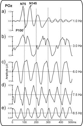
Pattern reversal VEP waveforms for upper left quadrant stimulation, showing the transition from transient to steady‐state response as a function of stimulation frequency (from 1–8.5 Hz). Note that the SSVEP waveform is primarily modulated at the pattern reversal rate, which is twice the rate of stimulation (considering there are two pattern reversals per full cycle of stimulation). At the slowest rate (1 Hz) the components of the transient VEP are clearly visible, including the N75, P100, and N145 components.
A major advantage of the SSVEP over the transient VEP is that the SSVEP signal is easily quantified in the frequency domain and can be rapidly extracted from background noise [Regan, 1989]. For example, recording the SSVEP at 6 or 8 Hz (the most commonly used temporal frequencies) produces a waveform with an adequate signal/noise ratio about 6 or 8 times faster than with transient stimulation. This makes the SSVEP an advantageous method under conditions of limited recording time, such as when studying infant vision [e.g., Morrone et al., 1996] or for clinical applications [e.g., Spinelli et al., 1994]. Besides these technical advantages, the SSVEP can be recorded under conditions that have a certain ecological validity, in that the flickering stimuli are continuously observable. In contrast, stimuli that elicit the transient VEP are displayed abruptly and then disappear. Thus, the SSVEP may provide relevant information about cortical activity patterns related to sustained visual experience. The amplitude of the SSVEP bears a close relationship with the psychophysical contrast threshold [e.g., Campbell and Maffei, 1979], and the SSVEP (and its magnetic field counterpart) is a sensitive index of perceptual rivalry [Brown and Norcia, 1997; Srinivasan et al., 1999] and visual selective attention [Chen et al., 2003; Di Russo et al., 1999a, b, 2001, 2002a; Hillyard et al., 1997; Morgan et al., 1996; Mueller et al., 1997, 1998a, b; Mueller and Hillyard, 2000; Pei et al., 2002].
An intrinsic disadvantage of SSVEP recordings, however, is that the rapid visual stimulation does not allow brain activity to return to a baseline state or “reset” before the next stimulus appears, so that the contributions of all visual areas overlap in the averaged waveform. In contrast, the transient VEP allows a chronometric analysis of the brain activity evoked in different cortical areas; this approach has benefited in recent years from the use of brain mapping and dipole modeling techniques. When the high temporal resolution of the VEP is combined with the high spatial resolution of functional MRI (fMRI), a well‐defined picture of the sequential activation of different visual‐cortical areas emerges [Di Russo et al., 2002b, 2005; Vanni et al., 2004]. The aim of the present study is to analyze the SSVEP in conjunction with fMRI in order to obtain information about its neural generators comparable to that previously reported for the transient VEP.
A number of studies based on electrophysiological [Hillyard et al., 1997; Mueller et al., 1998a; Pastor et al., 2003; Van Dijk and Spekreijse, 1990] and magnetoencephalographic (MEG) [Barnes et al., 2004; Fawcett et al., 2004; Mueller et al., 1997] recordings have attempted to identify the neural generators responsible for the surface‐recorded steady‐state evoked response. These studies found that the major contributions came from occipital brain regions, but specific visual‐cortical areas could not be identified with certainty. Fawcett et al. [2004], using MEG/MRI coregistration, were able to differentiate two separate sources of neural activity in medial occipital and lateral extrastriate visual cortex, respectively. However, while the medial occipital source showed enhanced oscillatory activity in response to repetitive stimulation, the lateral source actually showed reduced activity (desynchronization).
The lack of anatomical specificity in some of the previous electrophysiological and MEG studies was likely a consequence of methodological limitations such as a low number of recording sites and the type of stimuli used. With a sparse electrode array it is difficult to differentiate concurrent activity patterns arising from neighboring visual areas or to obtain an accurate picture of the voltage topography produced by a given source. Furthermore, the use of stimuli extending over wide visual angles is likely to activate large portions of the retinotopic cortical areas, thereby reducing the possibility of identifying the generator locations with precision. In particular, stimuli that span more than one visual quadrant (crossing the horizontal or vertical meridians) may activate neural populations with opposing geometry (as in the primary visual area), resulting in cancellation of concurrent electric fields and misinterpretation of the underlying source [Regan, 1989].
In the present study the SSVEP was recorded using a dense electrode array in response to focal stimulation in each of the visual quadrants. Sources were identified using dipole modeling based on a realistic head model, taking into account the loci of cortical activation revealed by fMRI in response to the same stimuli. These sources were also localized on flat maps with respect to visual cortical areas identified in individual subjects by retinotopic mapping and motion stimulation [Di Russo et al., 2005].
SUBJECTS AND METHODS
Subjects
Fifteen paid volunteer subjects (7 women; mean age, 25.7; range, 18–36 years) participated in the SSVEP recordings. A subset of 5 of these subjects (3 women; mean age, 26.2; range, 23–34 years) also received anatomical MRI scans and participated in the fMRI study. All subjects were right‐handed and had normal or corrected‐to‐normal visual acuity. Written, informed consent, approved by the local ethics committee, was obtained from all subjects after the procedures had been fully explained to them.
Stimuli
The stimulus consisted of a circular Gabor grating sinusoidally modulated in black and white and horizontally oriented; stimulus diameter was 2° of visual angle with a spatial frequency of 4 cycles/degree. The background luminance (22 cd/m2) was isoluminant with the mean luminance of the grating pattern, which was contrast modulated at 32%. The grating contrast reversed every 83.3 ms (reversal rate of 12 Hz) producing a complete cycle every 166.7 ms, so that the fundamental frequency was 6 Hz. The stimulus was presented in one quadrant at a time. Stimulus positions were centered along an arc that was equidistant (4°) from a central fixation point and located at polar angles of 25° above and 45° below the horizontal meridian, as described previously [Di Russo et al., 2002b, 2005].
Procedure
In the VEP experiment, the subject was comfortably seated in a dimly lit, sound‐attenuated, and electrically shielded chamber while stimuli were presented on a video monitor at a viewing distance of 114 cm. Subjects viewed the stimuli binocularly and were trained to maintain stable fixation on a central cross (0.2 × 0.2°) throughout stimulus presentation. Each run lasted 60 s followed by a 30‐s rest period, with longer breaks interspersed. A total of 16 runs was carried out in counterbalanced order to deliver at least 2,800 pattern‐reversal stimuli to each quadrant. The subjects were given feedback on their ability to maintain fixation.
Electrophysiological Recording and Data Analysis
The EEG was recorded using a BrainVision system (Germany) with 64 electrodes placed according to the 10‐10 system montage [see Di Russo et al., 2002b]. All scalp channels were referenced to the left mastoid (M1). Horizontal eye movements were monitored with a bipolar recording from electrodes at the left and right outer canthi. Blinks and vertical eye movements were recorded with an electrode below the left eye, which was referenced to site Fp1. The EEG from each electrode site was digitized at 1,000 Hz with an amplifier bandpass of 0.01–60 Hz including a 50 Hz notch filter and was stored for offline averaging. Computerized artifact rejection was performed prior to signal averaging in order to discard epochs in which deviations in eye position, blinks, or amplifier blocking occurred. On average, about 9% of the trials were rejected for violating these artifact criteria. VEPs were averaged separately for stimuli in each quadrant in epochs that began at the onset of each stimulus cycle and lasted for 1,000 ms. To further reduce high‐ and low‐frequency noise, the time‐averaged VEPs were bandpass‐filtered from 5 to 25 Hz.
SSVEP Topography
To visualize the voltage topography of the SSVEP, spline‐interpolated 3D maps were constructed for the dominant frequency response (second harmonic at 12 Hz), separately for stimulation in each quadrant. The 12 Hz waveform was extracted at each recording site by means of a fast Fourier transform of the averaged SSVEP over the 1,000‐ms epoch. The time‐varying 12 Hz amplitude (H) at each site was calculated as a function of response phase angle (α) according to: [H(12, α] = cos(α) Re(12) + sin(α) Im(12)], where Re(12) and Im(12) are the real and imaginary Fourier coefficients at 12 Hz. Amplitudes were calculated for alpha angles between 0 and 180° and were averaged across each successive 5° phase interval. The phase differences between successive topographies can directly be translated into time lags taking into account that for the 12‐Hz frequency one full period (360°) corresponds to 83.3 ms.
Modeling of SSVEP Sources
Multiple dipoles were fit sequentially to the spline interpolated scalp distributions of the original (not Fourier transformed) single‐subject and grand‐average SSVEP waveforms. Estimation of the dipolar sources of the SSVEP components was carried out using Brain Electrical Source Analysis (BESA 2000 v. 5.1; Megis Software, Germany), as described in more detail elsewhere [Di Russo et al., 2005]. This analysis used a realistic approximation of the head with the radius at the scalp surface obtained from the average of the group of subjects (87 mm). A spatial digitizer recorded the 3D coordinates of each electrode and of three fiducial landmarks (the left and right preauricular points and the nasion). The mean coordinates for each site averaged across all subjects were used for the topographic mapping and source localization procedures. In addition, individual spherical coordinates were related to the corresponding digitized fiducial landmarks and to landmarks identified on the standardized finite element model of BESA 2000.
Based on our previous study [Di Russo et al., 2005], a proximity seeding strategy was used to model the dipolar sources of the SSVEP. First, an unseeded model was fit over specific latency ranges (given below) to account for time‐varying patterns of SSVEP scalp topography. Next, loci of fMRI activation in close proximity to those dipoles were identified and were used to constrain the locations of the dipoles in a new seeded model. Single sources were constrained in location to the centers of the fMRI activations in primary (V1) and extrastriate visual areas and were adjusted in orientation over various time windows (given below) to obtain an optimal fit to the SSVEP topography. Both group and single‐subject analyses were conducted.
fMRI Protocols
Subjects (n = 5) were selected for participation in fMRI scanning on the basis of their ability to maintain steady visual fixation as assessed by electro‐oculographic recordings during the SSVEP sessions. The MR examinations were conducted at the Santa Lucia Foundation on a 1.5 T Siemens (Erlangen, Germany) MR scanner. Each subject performed three different fMRI protocols:
Steady‐state stimulation
In this procedure, 16 s of stimulation (pattern‐reversals) alternated with 16 s of no stimulation (pattern present but stationary) for eight cycles. This sequence was repeated at least three times for each quadrant. The visual stimulus was identical to that used in the VEP experiment.
Retinotopic mapping
Phase‐encoded stimuli were used to map the retinotopic organization of the cortical visual areas [Sereno et al., 1995; Tootell et al., 1997]. The stimuli consisted of high‐contrast flickering colored checks in either a ray‐ or a ring‐shaped configuration that varied slowly (1°/sec) in polar angle and eccentricity, respectively. These stimuli spared a central 0.75° circular zone of the visual field to avoid ambiguities caused by fixation instability.
MT mapping
Three additional scans were acquired to localize the motion‐sensitive area MT/V5 using the method of Tootell et al. [1995]. In a block design sequence, moving (7°/s) and stationary patterns (concentric, low‐contrast white rings surrounding the central fixation point on a light‐gray background, 0.2 cycles/degree, duty cycle = 0.2) were alternated in 32‐s epochs for 8 cycles/scan.
In all three experiments stimuli were presented on a backprojection screen and viewed with a mirror at an average distance of 21 cm. All stimuli were viewed passively, and subjects were only required to maintain stable fixation throughout the period of scan acquisition. Head motion was minimized by using a bite bar with an individually molded dental impression as described elsewhere [Sereno et al., 2001]. This system provided a marked reduction in motion artifacts without introducing any discomfort. Subjects' heads were also stabilized with foam pads. Interior surfaces were covered with black velvet to eliminate reflections.
fMRI Scanning
Single‐shot echo‐planar imaging (EPI) images were collected using a Small Flex quadrature surface RF coil placed over the occipital and parietal areas. MR slices were 4 mm thick, with an in‐plane resolution of 3 × 3 mm and oriented approximately perpendicular to the calcarine fissure. Each scan had a duration of either 256 sec (for the two‐condition procedures: steady‐state and MT+ mapping), or 512 sec (for retinotopy), with TR = 2000 or 4000 ms, respectively. Each scan included 128 or 256 single‐shot EPI images per slice in 16 to 32 contiguous slices (TE = 42, flip angle = 90, 64 × 64 matrix, bandwidth = 926 Hz/pixel). In each scan the first 8 s of the acquisition were discarded from data analysis in order to achieve a steady state. To increase signal to noise, data were averaged over three scans for each stimulus type (eccentricity, polar angle, MT mapping, and steady‐state quadrant stimulation). A total of 105 functional scans were carried out on the five subjects (30 scans to map the retinotopic visual areas, 15 scans to map MT/V5, and 60 scans for the steady‐state quadrant stimulation). The cortical surface for each subject was reconstructed from a pair of structural scans (T1‐weighted MPRAGE, TR = 11.4 ms, TE = 4.4 ms, flip angle = 10, 1 × 1 × 1 mm resolution) taken in a separate session using a head coil. The last scan of each functional session was an alignment scan (also MPRAGE, 1 × 1 × 1 mm or 1 × 1 × 2 mm) acquired with the surface coil in the plane of the functional scans. The alignment scan was used to establish an initial registration of the functional data with the surface. Additional affine transformations that included a small amount of shear were then applied to the functional scans for each subject using blink comparison with the structural images to achieve an exact overlay of the functional data onto each cortical surface.
Single‐subject data analysis
Processing of functional and anatomical images was performed using FreeSurfer [Dale et al., 1999; Fischl et al., 1999]. Data from two‐condition experiments and phase‐encoded retinotopic experiments were analyzed by means of a Fourier transform (FT) of the MR time course from each voxel after removing constant and linear terms. This generated a vector with real and imaginary components for each frequency that defined an amplitude and phase of the periodic signal at that frequency. To estimate the significance of correlation of blood oxygenation level‐dependent (BOLD) signal with the stimulus frequency (8 cycles per scan), the squared amplitude of the signal at the stimulus frequency was divided by the mean of squared amplitudes at all other “noise” frequencies (excluding low‐frequency signals due to residual head motion and harmonics of the stimulus frequency). This ratio of two chi‐squared statistics follows the F‐distribution with degrees of freedom equal to the number of time points and can be used to calculate a significance P‐value. This procedure has been used in many previous studies [e.g., Tootell et al., 1997]. Above a minimum threshold, the statistical significance levels of the displayed pseudocolor ranges were normalized according to the overall sensitivity of each subject, as described elsewhere [Hadjikhani et al., 1998]. All effects were analyzed and displayed in cortical surface format [Felleman and Van Essen, 1991; Schiller and Dolan, 1994], which made it possible to extract the MR time courses from voxels in specific cortical areas (V1, V2, V3/VP, V3A, V4v, and MT/V5). The boundaries of the retinotopic visual areas were defined in each participant on the basis of the field‐signs calculated from the maps of polar angle and eccentricity [Sereno et al., 1995].
Group data analysis
Group data analyses were performed with SPM99 (Wellcome Department of Cognitive Neurology, London, UK). Functional images from each participant were coaligned with the high‐resolution anatomical scan (MPRAGE) taken in the same session. Images were motion‐corrected through a rigid body transformation with a least‐squares approach and transformed into normalized stereotaxic space [Talairach and Tournoux, 1998] using a nonlinear stereotaxic normalization procedure [Friston et al., 1995] with the SPM99 software platform. The template image was based on average data provided by the Montreal Neurological Institute (MNI) [Mazziotta et al., 1995]. A fixed‐effects general linear model was employed to compute statistical maps for the group average. The experimental conditions were modeled as simple boxcar functions (stimulus vs. baseline) and convolved with a synthetic hemodynamic response function. Statistical significance of activated regions was assessed using a probability criterion of P ≤ 0.01 uncorrected at the voxel level and P < 0.01 corrected at the cluster level. The statistical parametric maps were superimposed onto the standard brain supplied by SPM99 and flattened with the FreeSurfer software.
RESULTS
SSVEP Waveforms and Topography
The grand‐averaged SSVEP waveforms elicited at selected electrode sites by stimuli in each of the four quadrants are shown in Figure 2a. The waveforms were sinusoidal in form and modulated at 12 Hz (the contrast reversal rate), with maximal amplitude over midline parieto‐occipital electrodes. At these midline sites (e.g., POz) the SSVEP phase (α) was similar for left and right stimuli in both upper (mean phase difference (Δα) = 20°) and lower (Δα = 25°) visual quadrants. In contrast, large phase differences were produced by upper vs. lower quadrant stimulation in both left (Δα = 230°) and right (Δα = 210°) visual fields. At the lateral recording sites (I5/I6, PO3/PO4) the SSVEP amplitudes were generally larger over the contralateral than the ipsilateral hemisphere and showed large regional variations in response phase. A similar spatiotemporal configuration is shown for a typical individual subject in Figure 2b; the mean phase shift at POz was 15° for left vs. right field stimulation and 210° for upper vs. lower quadrant stimuli.
Figure 2.
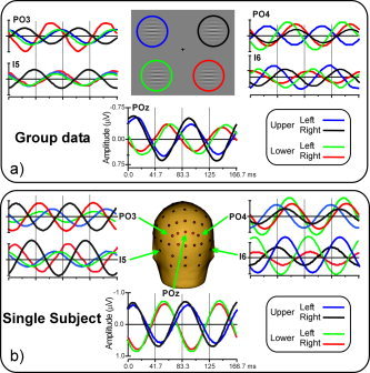
Grand averaged SSVEP waveforms to pattern reversal stimuli located in the upper‐left (blue), upper‐right (black), lower‐left (green), and lower‐right (red) quadrants of the visual field. Each quadrant was stimulated separately. Recordings are from parieto‐occipital (PO3, POz, and PO4), and occipito‐temporal (I5 and I6) sites as indicated on the head icon. Stimulus locations are shown schematically at top. a: Group data. b: Single‐subject data.
The scalp topography of the SSVEP varied systematically as a function of response phase, which indicated that more than one generator source was contributing to the waveform. Figure 3a illustrates the sequential changes in topography in response to the upper right quadrant stimulus. For upper quadrant stimulation the voltage field showed a unitary negative focus over the medial occipito‐parietal scalp during the phase range 0°–40°, consistent with a radially oriented medial dipolar source. At 80°–120° the negative field shifted inferiorly, with a contralateral positive focus over the occipito‐temporal region and a more medial negative focus, consistent with a lateralized, tangential dipolar source. For lower quadrant stimulation (Fig. 3b,c) the topography showed a unitary positive focus over the medial occipital scalp over 20°–60° and a more contralateral focus at 80°–120°, consistent with two separate radially oriented sources. The SSVEP topographies over these critical phase ranges were very similar for the group‐averaged (Fig. 3b) and single‐subject data (Fig. 3c). The topographies over the 180°–360° phase range (not shown) were virtually identical to those produced over 0°–180° but were reversed in polarity.
Figure 3.
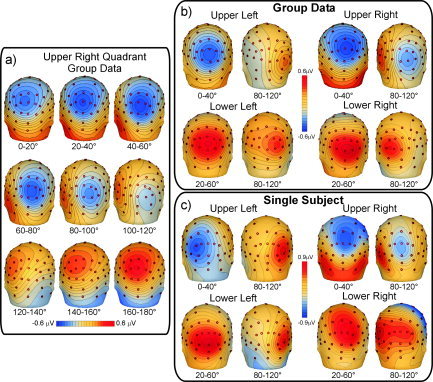
Spline‐interpolated voltage topography of the 12 Hz SSVEP. a: Sequential topographies elicited by stimuli in upper right quadrant (group‐averaged data). Intervals of response phase (in degrees) are equivalent to successive time periods throughout one cycle of the 12 Hz waveform, and zero phase is taken arbitrarily as the time of contrast shift. b: Scalp topographies of the group‐averaged data to stimuli in each quadrant over the early and late phase ranges at which the topographies differed maximally from one another. c: Same as b for single‐subject data.
Dipole Model without fMRI Constraints
Inverse dipole modeling of the SSVEP generators was carried out on the grand‐average and single subject waveforms using the BESA 2000 software (Fig. 4). Separate unseeded models (without fMRI constraints) were calculated for each of the four quadrants using the following strategy: (1) A single dipole was fit over the phase ranges 0°–40° and 20°–60° for upper and lower quadrants, respectively, which accounted for the medial topographies shown in Figure 3. These dipoles were oriented radially and localized to medial posterior occipital cortex (Fig. 4a; Table I). (2) A second dipole was fit over the 80°–120° range for all quadrants to account for the more lateralized voltage topography in this interval. These dipoles were localized more laterally in the occipital cortex. For all quadrants these two‐dipole models accounted for around 97% of the variance in scalp voltage topography over the time range 0–167 ms (Table II). Unseeded modeling of the single‐subject topographies shown in Figure 4b produced similar dipole localizations with residual variances that averaged around 4%.
Figure 4.
Unseeded dipole source models accounting for the SSVEP voltage topographies in each quadrant. Source waveforms at the left of each head‐icon show the time course of voltage contributed by each dipole. Polarity convention: negativity at pointed end of dipole plotted upwards. a: Model based on group averaged waveforms. b: Model based on single subject's waveforms.
Table I.
Talairach coordinates of the medial and lateral occipital dipoles in the unseeded source model (values are in mm)
| Group data: x, y, z | Single subject: x, y, z | |
|---|---|---|
| Upper left | ||
| Medial | 13,−92,−9 | 4,−82,−6 |
| Lateral | 36,−71,−4 | 35,−78,3 |
| Lower left | ||
| Medial | 5,−74,2 | 7,−83,11 |
| Lateral | 38,−65,0 | 39,−68,−3 |
| Upper right | ||
| Medial | −9,−86,−7 | −16,−85,−1 |
| Lateral | −35,−73,−5 | −37,−79,−2 |
| Lower right | ||
| Medial | −6,−80,3 | −10,−81,5 |
| Lateral | −31,−64,8 | −40,−74,6 |
Table II.
Residual variance percentages of source models over one full stimulus cycle (0‐167 ms)
| Source model | UL | UR | LL | LR |
|---|---|---|---|---|
| Unseeded 2‐dipole model | 2.7 | 3.1 | 2.8 | 3.0 |
| Seeded 2‐dipole, (V1 and MTS) | 2.9 | 3.4 | 3.2 | 3.2 |
| Seeded 4‐dipole, (V1, MTS, pIPS, and CoS) | 2.0 | 2.3 | 2.2 | 2.0 |
UL, UR, LL, and LR refer to upper‐left, upper‐right, lower‐left, and lower‐right visual quadrants. Group‐averaged data.
fMRI Activations
In the group‐averaged data, sensory‐evoked fMRI activations were observed in multiple visual cortical areas of the contralateral hemisphere. These included regions of the calcarine fissure, the middle temporal sulcus, the inferior occipital cortex (fusiform gyrus and collateral sulcus), and the middle occipital gyrus in and around the posterior intraparietal sulcus (pIPS). This posterior limb of the IPS enters the occipital lobe, and reportedly extends up to visual areas V3A [Tootell et al., 1997] and V7 [Tootell et al., 1998]. Figure 5a shows the contralateral activations produced by stimuli in each quadrant superimposed on the left and right flattened cortical surfaces of the MNI template. When the upper visual fields were stimulated the activations were more prominent in ventral cortical areas (the lower bank of the calcarine fissure and the collateral sulcus/fusiform region), while for lower visual field stimulation activations were produced within the upper bank of the calcarine fissure as well as in a ventral region located in the fusiform gyrus (Table III). Both upper and lower field stimuli activated the mid‐occipital (pIPS) and mid‐temporal regions.
Figure 5.
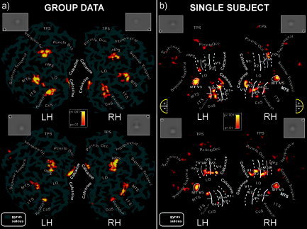
a: Group‐averaged contralateral fMRI activations for the four quadrants superimposed on the flattened left and right hemispheres of the MNI template. Logo next to each flat map indicates the visual quadrant stimulated. The pseudocolor scale at the center indicates the significance of the activations. Major sulci (dark gray) are labeled as follows: parieto‐occipital sulcus (Parieto Occ.), transverse segment of the parietal sulcus (TPS), posterior intraparietal sulcus (pIPS), lateral occipital sulcus (LO), collateral sulcus (CoS), superior temporal sulcus (Superior Temporal), middle temporal sulcus (MTS), inferior temporal sulcus (ITS), fusiform gyrus (Fusiform), and calcarine fissure (Calcarine). b: Flattened left and right hemispheres of an individual participant showing contralateral activations in response to pattern‐reversal stimulation of the four quadrants. Boundaries of the classic visual areas were defined by mapping the “visual field sign” and motion sensitivity (for MT/V5) (see Subjects and Methods). As indicated in the semicircular logo, dashed and solid lines correspond to vertical and horizontal meridians, respectively, and plus and minus symbols refer to upper and lower visual field representations, respectively. The scale in the center indicates the significance of the activations.
Table III.
Talairach coordinates of the significant striate and extrastriate contralateral activation sites in the group‐averaged and single‐subject fMRI data
| Group data: x, y, z | Single subject: x, y, z | |
|---|---|---|
| Upper left | ||
| Calcarine (V1+) | 9, −88, −6 | 11, −87, −5 |
| MTS (MT/V5) | 44, −69, 1 | 45, −68, 6 |
| pIPS (V3A+) | 35, −75, 24 | 30, −80, 28 |
| CoS/Fus (V4v, V4/V8+) | 27, −71, −11 | 22, −70, −13 |
| Lower left | ||
| Calcarine (V1−) | 12, −90, 9 | 10, −92, 11 |
| MTS (MT/V5) | 46, −69, 3 | 43, −66, 2 |
| pIPS (V3A−) | 29, −80, 16 | 28, −71, 16 |
| CoS/Fus (V4/V8−) | 30, −70, −15 | 22, −69, −10 |
| Upper right | ||
| Calcarine (V1+) | −7, −90, −3 | −8, −92, −2 |
| MTS (MT/V5) | −42, −71, 0 | −43, −66, 4 |
| pIPS (V3A+) | −32, −79, 26 | −28, −85, 20 |
| CoS/Fus (V4v, V4/V8+) | −23, −75, −6 | −40, −59, −12 |
| Lower right | ||
| Calcarine (V1−) | −10, −89, 12 | −7, −87, 11 |
| MTS (MT/V5) | −45, −70, 3 | −43, −66, 3 |
| pIPS (V3A−) | −33, −86, 17 | −28, −88, 16 |
| CoS/Fus (V4/V8−) | −29, −78, −11 | −37, −56, −7 |
Coordinates of activations are given for stimuli in each of the four quadrants (values are in mm). For abbreviations, see Figure 5 legend.
Stimulus‐evoked fMRI activations were localized for each subject with respect to the retinotopically organized visual areas defined on the basis of their field signs [Sereno et al., 1995] and with respect to area MT/V5 defined by motion stimulation. The borders of retinotopically organized visual areas (V1, V2, V3, VP, V3A, and V4v) and area MT/V5 could be identified for each subject, and activations in striate and adjacent extrastriate visual areas could be distinguished despite their close proximity and individual differences in cortical anatomy. As shown in Figure 5b for a typical subject, upper quadrant stimuli produced activations in the lower banks of areas V1 and V2 as well as in areas VP, V4v, V3A+, and MT/V5. Lower quadrant stimuli produced activations in the upper banks of V1 and V2, and in areas V3, V3A‐, and MT/V5.
Activations were also observed in a ventral visual area just anterior to the horizontal meridian representation marking the anterior border of area V4v [Sereno et al., 1995]. Anatomically, this area was located within the collateral sulcus and extended onto the fusiform gyrus. This ventral area most likely corresponds to the color‐sensitive area that has been called either V4 [Lueck et al., 1989; Zeki and Bartels, 1999] or V8 [Hadjikhani et al., 1998; Tootell et al., 2001]. To avoid controversy, this area will herein be designated V4/V8. Like dorsal V3A, this ventral area represents the entire contralateral hemifield, with superior and inferior portions (on the flat map) responding to lower (−) and upper (+) visual field stimulation, respectively [Hadjikhani et al., 1998; see also Di Russo et al., 2001, 2005]. Activation of this ventral visual area was also evident in the group data shown in Figure 5a.
On the basis of individual single‐subject mappings, the group‐averaged fMRI activations produced by steady‐state stimulation may be assigned to specific visual areas. The group activations in the calcarine region appear to originate primarily from area V1, although contributions from the adjacent area V2 are also possible. The mid‐occipital activations in the group data correspond to activity in dorsal area V3A, while the mid‐temporal activations originate in the motion‐sensitive area MT/V5. Finally, the group activations in the fusiform gyrus and collateral sulcus appear to correspond to ventral areas V4v and V4/V8. The Talairach coordinates at the centers of these clusters of activation are given in Table III.
fMRI Constrained Dipole Modeling
There was a good correspondence between the calculated locations of the dipoles in the unseeded model and the loci of fMRI activation produced by the same stimuli (cf. Tables I and III). The medial occipital dipoles accounting for the early phase of the SSVEP were in close proximity to the calcarine (V1) activations found with fMRI; the mean disparity between the dipole positions and fMRI activations was 5, 8, and 4 mm in the X, Y, and Z dimensions, respectively. A good correspondence was also found between the locations of the lateral occipital dipoles fit to the later phase of the SSVEP and the mid‐temporal (MT/V5) activations. The mean disparity was 7, 6, and 4 mm in the X, Y, and Z dimensions, respectively.
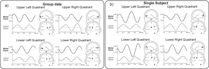
For the seeded (fMRI constrained) 2‐dipole model of the group data the medial and lateral occipital dipole positions were shifted to correspond to the locations of the fMRI foci of activation V1 and MT/V5, respectively (Table III) and were fit only in orientation within the same time windows as for the unseeded model. This seeded model yielded a mean residual variance of 3.2% (averaged over the four quadrants), only slightly greater than for the unseeded model (2.9%) (Table II). While this 2‐dipole seeded model accounted for nearly all the variance in scalp topography of the SSVEP, a 4‐dipole seeded model was also constructed to evaluate possible contributions from the other active sites identified with fMRI. In this model two additional dipoles were placed at the pIPS (V3A) and collateral sulcus (V4v, V4/V8) activation sites, respectively, and were fit only in orientation. This 4‐dipole model accounted for 97–98% of the scalp potential variance for stimulation in the different quadrants (Table. II). Comparing the source waveforms of the three different dipole models, the phases and the relative amplitudes of the medial (V1) and lateral (MT/V5) occipital sources varied minimally, which supports the robustness of the modeling procedures.
In the seeded 4‐dipole models of the group data (Fig. 6a), it can be seen that the source waveforms of the medial occipital (V1) dipole were very similar in phase to the scalp‐recorded activity at POz. These source waveforms also showed a polarity inversion between upper vs. lower field stimuli of ∼180°. The dipole seeded to area MT/V5 had a source waveform with a phase delay of about 40–60° ms with respect to the V1 dipole. The dipoles seeded to the mid‐occipital (V3A) location had source waveforms shifted by around 20–40° later than those of MT/V5. Finally, the dipoles seeded to the ventral occipital activations (V4/V8) had source waveforms that were delayed by 60–80° with respect to the MT/V5 dipole. Source analysis of the single subject's data yielded similar results (Fig. 6b).
Figure 6.
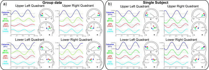
Four‐dipole source models in which dipole locations were seeded to the loci of fMRI activation for each quadrant. Models were based on (a) group‐averaged and (b) individual subject data. The waveforms at the left of each head‐icon indicate the time course of activity of each dipole (source waveforms). Sources are labeled according the seeded fMRI areas.
In Table IV the phase differences of the various seeded sources with respect to V1 are reported, with phase differences converted into time differences. This allows a comparison of the sequence of activation in different cortical regions as determined from the SSVEP with the corresponding sequence determined from the pattern‐reversal transient VEP in a previous study [Di Russo et al., 2005] that used identical stimuli but a slower rate. The SSVEP phase differences correspond well with the timing of the transient VEP components that were localized to the same cortical regions, suggesting a similar spatiotemporal sequence of activation for the two types of stimulation. It should be cautioned, however, that timing information cannot be precisely defined using SSVEPs, because different portions of the SSVEP waveform may be evoked by different preceding stimuli in the repetitive sequence.
Table IV.
Time sequence of cortical activation derived from SSVEP and transient VEP recordings (transient data are from Di Russo et al., 2005)
| SSVEPs | Transient VEPs | ||
|---|---|---|---|
| Onset | Peak | ||
| Modeled sources for upper quadrant stimuli | |||
| MTS (MT/V5) | 20 | 20 | 20 |
| pIPS (V3A+) | 38 | 41 | 50 |
| CoS/Fus (V4v, V4/V8+) | 64 | 75 | 88 |
| Modeled sources for lower quadrant stimuli | |||
| MTS (MT/V5) | 22 | 20 | 20 |
| pIPS (V3A−) | 42 | 40 | 46 |
| CoS/Fus (V4/V8−) | 65 | 71 | 85 |
Table shows time delays (expressed in ms) between neural activity in V1 and subsequent activity in the other cortical areas. For the SSVEP, phase differences were transformed to time differences (see Subjects and Methods). Group‐averaged data.
DISCUSSION
The present study used dipole modeling in conjunction with fMRI to analyze the neural generators of the SSVEP elicited by a 6‐Hz pattern‐reversing stimulus (producing a 12‐Hz contrast reversal rate). The results indicated that the SSVEP originates primarily from two concurrently active dipolar sources that were situated in medial and lateral occipital cortex, respectively, and were 40°–60° out of phase. The medial occipital source was located in close proximity to a focal zone of neural activation in area V1 that was produced by the same stimuli in a separate session with fMRI. When seeded to this site of V1 activation, the dipole showed a near 180° phase inversion for upper vs. lower visual field stimulation, consistent with the cruciform geometry of the primary visual cortex [e.g., Di Russo et al., 2001, 2005]. These observations provide strong evidence that phase‐locked neural activity in area V1 is a major contributor to the pattern‐reversal SSVEP. The second principal source was localized more laterally, close to a zone of activation seen with fMRI in the mid‐temporal motion‐sensitive area MT/V5. Together, these two main sources accounted for about 97% of the time‐varying topography of the SSVEP.
Two additional sites of neural activation in response to the pattern‐reversing stimulus were identified with fMRI in mid‐occipital (area V3A) and ventral occipital (areas V4v/V4/V8) regions. Additional dipoles seeded to these zones of activation produced only a modest improvement in accounting for the SSVEP topography, however, suggesting that these cortical areas make only minor contributions to the scalp‐recorded SSVEP. Nonetheless, the phase relationships among the four seeded dipoles suggest a temporal sequence of activation in the different visual areas that is consistent with that observed for the transient VEP elicited by identical stimuli presented at a slower rate [Di Russo et al., 2005]. The inferred sequence of activation for stimulation of the upper visual fields was V1+, MT/V5, V3A+, V4v, V4/V8+ and for the lower fields was V1−, MT/V5, V3A−, V4/V8−. In some of the single subjects fMRI also showed activity in areas V2 and V3, but due to their close proximity these areas were included in the V1 and V3A sources, respectively, in the group analysis.
Previous studies that estimated the neural sources of the SSVEP (or its magnetic field counterpart) using single‐dipole models found the principal generators to be situated in occipital regions [Mueller et al., 1997; Van Dijk and Spekreijse, 1990], and the dipole localization depended on stimulation frequency [Mueller et al., 1997]. More specifically, a major source in primary visual cortex was inferred by Pastor et al. [2003] for the SSVEP to unpatterned flickering stimuli on the basis of combined electrophysiological recordings and positron emission tomography. A study by Hillyard et al. [1997] combined dipole‐modeling techniques with fMRI to support a lateral occipital source for the attentional modulation of the 8–12 Hz SSVEP, but the generators of the SSVEP itself were not examined. Using a different modeling approach that estimates intracranial current densities, Mueller et al. [1998] concluded that the attentional modulation of higher frequency (20–28 Hz) SSVEP activity was localized in dorsal occipito‐parietal cortex.
Most relevant to the present study, a recent MEG study by Fawcett et al. [2004] examined the frequency‐specific oscillatory power changes produced in the cortex by repetitive visual stimulation using the event‐related synchronization and desynchronization (ERS and ERD) technique. The stimuli used were pattern‐reversing checkerboards presented to left and right parafoveal regions at various temporal frequencies. In a first experiment using square‐wave modulated checkerboards, Fawcett et al. [2004] found an ERS peak that was localized to the contralateral medial occipital cortex using synthetic aperture magnetometry. In a second experiment that used sinusoidally modulated checkerboards (as in the present study), they found two distinct patterns of activity: one peak of ERS was localized mainly to the contralateral medial occipital cortex, while a second peak of ERD was observed in lateral extrastriate areas that may include the lateral occipital and V5/MT complexes.
The present study was the first to our knowledge to systematically investigate the neural generators of the electrocortical response to repetitive pattern reversal stimulation (i.e., the SSVEP). Our spatiotemporal analysis found that at least two dipolar sources were necessary to account adequately for the time‐varying SSVEP topography, which were situated in medial and lateral regions of the visual cortex, respectively. On the basis of converging fMRI evidence in conjunction with retinotopic mapping, we were able to localize these sources with some confidence to visual areas V1 and MT/V5, respectively. The localization of the medial occipital source to area V1 was further confirmed by showing its polarity inversion for upper vs. lower visual field stimulation, in accordance with the cruciform model [see Di Russo et al., 2002b]. It seems likely that the medial occipital source identified by Fawcett et al. [2004] for the magnetic counterpart of the SSVEP also included generator activity in primary visual cortex.
It should be cautioned that the use of hemodynamic imaging to substantiate the estimated locations of ERP sources is subject to certain caveats [for similar considerations, see Bonmassar et al., 2001; Di Russo et al., 2001, 2003, 2005; Heinze et al., 1994; Mangun et al., 2001; Martinez et al., 1999, 2001b; Snyder et al., 1995; Vanni et al., 2004]. First and foremost is the assumption that the hemodynamic response obtained with fMRI or PET is driven by the same neural activity that gives rise to the ERP. With regard to visual‐evoked activity, such correspondence appears to be optimal in humans for medial occipital cortex (including the calcarine region) and is less consistent for extrastriate visual areas [Gratton et al., 2001]. Despite this caveat, several considerations lend support to the validity of the present dipole modeling approach. First, small stimuli like those used here reportedly activate small, punctuate zones in the early visual areas, extending across only a small portion of a gyrus or sulcus [Tootell et al., 1998]. This makes it reasonable to model the source for a single visual area (or for two retinotopically aligned visual areas) as a single dipole. Second, the representations of a particular location in the visual field in several adjoining visual areas are often close to each other (e.g., upper visual field representation in V4v and VP or lower visual field representation in V2 and V3). While this makes it difficult to distinguish the individual contributions of adjoining areas, it also makes it appropriate to collapse their combined activity into a single source. Third, the number of dipoles chosen to fit the VEP was primarily determined by the number of topographically distinctive components in the waveform rather than by an arbitrary criterion of goodness of fit.
In summary, the present study combined SSVEP recording with structural and functional MRI and retinotopic mapping of visual cortical areas to analyze the generators of phase‐locked neural activity elicited by a 6‐Hz pattern‐reversal stimulus. Two major sources having different phase relationships with respect to the repetitive stimulation were identified and were colocalized with neural activity in primary visual cortex and in the motion‐sensitive area MT/V5. Additional stimulus‐evoked activity observed with fMRI in mid‐occipital (area V3A) and ventral occipital (area V4/V8) regions only appears to make minor contributions to the surface recorded SSVEP. This analysis should enhance the utility of the SSVEP both as a clinical tool for rapidly assessing the functioning of specific visual‐cortical regions and as an investigative tool for studying the cortical mechanisms of visual‐perceptual processing.
REFERENCES
- Barnes GR, Hillebrand A, Fawcett IP, Singh KD (2004): Realistic spatial sampling for MEG beamformer images. Hum Brain Mapp 23: 120–127. [DOI] [PMC free article] [PubMed] [Google Scholar]
- Bonmassar G, Hadjikhani N, Ives JR, Hinton D, Belliveau JW (2001): Influence of EEG electrodes on the BOLD fMRI signal. Hum Brain Mapp 14: 108–115. [DOI] [PMC free article] [PubMed] [Google Scholar]
- Brown RJ, Norcia AM (1997): A method for investigating binocular rivalry in real‐time with the steady‐state VEP. Vision Res 37: 2401–2408. [DOI] [PubMed] [Google Scholar]
- Campbell FW, Maffei L (1970): Electrophysiological evidence for the existence of orientation and size detectors in the human visual system. J Physiol 207: 635–652. [DOI] [PMC free article] [PubMed] [Google Scholar]
- Campbell FW, Maffei L (1979): Stopped visual motion. Nature 278: 192. [DOI] [PubMed] [Google Scholar]
- Campbell FW, Robson JG (1968): Application of Fourier analysis to the visibility of gratings. J Physiol 197: 551–566. [DOI] [PMC free article] [PubMed] [Google Scholar]
- Chen Y, Seth AK, Gally JA, Edelman GM (2003): The power of human brain magnetoencephalographic signals can be modulated up or down by changes in an attentive visual task. Proc Natl Acad Sci U S A 100: 3501–3506. [DOI] [PMC free article] [PubMed] [Google Scholar]
- Dale AM, Fischl B, Sereno MI (1999): Cortical surface‐based analysis. I. Segmentation and surface reconstruction. Neuroimage 9: 179–194. [DOI] [PubMed] [Google Scholar]
- Di Russo F, Spinelli D (1999a): Electrophysiological evidence for an early attentional mechanism in visual processing in humans. Vision Res 39: 2975–2985. [DOI] [PubMed] [Google Scholar]
- Di Russo F, Spinelli D (1999b): Spatial attention has different effects on the magno‐ and parvo‐cellular pathways. Neuroreport 10: 2755–2762. [DOI] [PubMed] [Google Scholar]
- Di Russo F, Spinelli D, Morrone MC (2001): Automatic gain control contrast mechanisms are modulated by attention in humans: evidence from visual evoked potentials. Vision Res 41: 2435–2447. [DOI] [PubMed] [Google Scholar]
- Di Russo F, Teder‐Sälejärvi WA, Hillyard SA (2002a): Steady‐state VEP and attentional visual processing In: Zani A, Proverbio AM, editors. The Cognitive Electrophysiology of Mind and Brain. New York: Academic Press; p 259–274. [Google Scholar]
- Di Russo F, Martínez A, Sereno MI, Pitzalis S, Hillyard SA (2002b): The cortical sources of the early components of the visual evoked potential. Hum Brain Mapp 15: 95–111. [DOI] [PMC free article] [PubMed] [Google Scholar]
- Di Russo F, Martínez A, Hillyard SA (2003): Source analysis of event‐related cortical activity during visuo‐spatial attention. Cereb Cortex 13: 486–499. [DOI] [PubMed] [Google Scholar]
- Di Russo F, Pitzalis S, Spitoni G, Aprile T, Patria F, Spinelli D, Hillyard SA (2005): Identification of the neural sources of the pattern‐reversal VEP. Neuroimage 24: 874–886. [DOI] [PubMed] [Google Scholar]
- Fawcett IP, Barnes GR, Hillebrand A, Singh KD (2004): The temporal frequency tuning of human visual cortex investigated using synthetic aperture magnetometry. Neuroimage 21: 1542–1553. [DOI] [PubMed] [Google Scholar]
- Felleman DJ, Van Essen DC (1991): Distributed hierarchical processing in the primate cerebral cortex. Cereb Cortex 1: 1–47. [DOI] [PubMed] [Google Scholar]
- Fischl B, Sereno MI, Dale AM (1999): Cortical surface‐based analysis. II. Inflation, flattening, and a surface‐based coordinate system. Neuroimage 9: 195–207. [DOI] [PubMed] [Google Scholar]
- Friston KJ, Frith CD, Turner R, Frackowiak RS (1995): Characterizing evoked hemodynamics with fMRI. Neuroimage 2: 157–165. [DOI] [PubMed] [Google Scholar]
- Gratton G, Goodman‐Wood MR, Fabiani M (2001): Comparison of neuronal and hemodynamic measures of the brain response to visual stimulation: an optical imaging study. Hum Brain Mapp 13: 13–25. [DOI] [PMC free article] [PubMed] [Google Scholar]
- Hadjikhani N, Liu AK, Dale AM, Cavanagh P, Tootell RB (1998): Retinotopy and color sensitivity in human visual cortical area V8. Nat Neurosci 1: 235–241. [DOI] [PubMed] [Google Scholar]
- Heinze HJ, Mangun GR, Burchert W, Hinrichs H, Scholz M, Muente TF, Goes A, Scherg M, Johannes S, Hundeshagen H, Gazzaniga MS, Hillyard SA. (1994): Combined spatial and temporal imaging of brain activity during visual selective attention in humans. Nature 372: 543–546. [DOI] [PubMed] [Google Scholar]
- Hillyard SA, Hinrichs H, Tempelmann C, Morgan ST, Hansen JC, Scheich H, Heinze HJ (1997): Combining steady‐state visual evoked potentials and fMRI to localize brain activity during selective attention. Hum Brain Mapp 5: 287–292. [DOI] [PubMed] [Google Scholar]
- Lueck CJ, Zeki S, Friston KJ, Deiber MP, Cope P, Cunningham VJ, Lammertsma AA, Kennard C, Frackowiak RS (1989): The colour centre in the cerebral cortex of man. Nature 340: 386–389. [DOI] [PubMed] [Google Scholar]
- Mangun GR, Hinrichs H, Scholz M, Mueller‐Gaertner HW, Herzog H, Krause BJ, Tellman L, Kemna L, Heinze HJ (2001): Integrating electrophysiology and neuroimaging of spatial selective attention to simple isolated visual stimuli. Vision Res 41: 1423–1435. [DOI] [PubMed] [Google Scholar]
- Martinez A, Anllo‐Vento L, Sereno MI, Frank LR, Buxton RB, Dubowitz DJ, Wong EC, Hinrichs H, Heinze HJ, Hillyard SA (1999): Involvement of striate and extrastriate visual cortical areas in spatial attention. Nat Neurosci 2: 364–369. [DOI] [PubMed] [Google Scholar]
- Martinez A, Di Russo F, Anllo‐Vento L, Hillyard SA (2001a): Electrophysiological analysis of cortical mechanisms of selective attention to high and low spatial frequencies. Clin Neurophysiol 112: 1980–1998. [DOI] [PubMed] [Google Scholar]
- Martinez A, Di Russo F, Anllo‐Vento L, Sereno MI, Buxton RB, Hillyard SA (2001b): Putting spatial attention on the map: timing and localization of stimulus selection processes in striate and extrastriate visual areas. Vision Res 41: 1437–1457. [DOI] [PubMed] [Google Scholar]
- Mazziotta JC, Toga AW, Evans AC, Fox PT, Lancaster JL (1995): Digital brain atlases. Trends Neurosci 18: 210–211. [DOI] [PubMed] [Google Scholar]
- Morgan ST, Hansen JC, Hillyard SA (1996): Selective attention to stimulus location modulates the steady state visual evoked potential. Proc Natl Acad Sci U S A 93: 4770–4774. [DOI] [PMC free article] [PubMed] [Google Scholar]
- Morrone MC, Fiorentini A, Burr DC (1996): Development of the temporal properties of visual evoked potentials to luminance and colour contrast in infants. Vision Res 36: 3141–3155. [DOI] [PubMed] [Google Scholar]
- Mueller MM, Hillyard S (2000): Concurrent recording of steady‐state and transient event‐related potentials as indices of visual‐spatial selective attention. Clin Neurophysiol 111: 1544–1552. [DOI] [PubMed] [Google Scholar]
- Mueller MM, Teder‐Salejarvi W, Hillyard SA (1997): Magnetoencephalographic recording of steady‐state visual evoked cortical activity. Brain Topogr 9: 163–168. [DOI] [PubMed] [Google Scholar]
- Mueller MM, Picton TW, Valdes‐Sosa P, Riera P, Teder‐Salejarvi W, Hillyard SA (1998a): Effects of spatial selective attention on the steady‐state visual evoked potential in the 20‐28 Hz range. Cogn Brain Res 6: 249–261. [DOI] [PubMed] [Google Scholar]
- Mueller MM, Teder‐Salejarvi W, Hillyard SA (1998b): The time course of cortical facilitation during cued shifts of spatial attention. Nat Neurosci 1: 631–634. [DOI] [PubMed] [Google Scholar]
- Pastor MA, Artieda J, Arbizu J, Valencia M, Masdeu JC (2003): Human cerebral activation during steady‐state visual‐evoked responses. J Neurosci 17: 11621–11627. [DOI] [PMC free article] [PubMed] [Google Scholar]
- Pei F, Pettet MW, Norcia AM (2002): Neural correlates of object‐based attention. J Vis 2: 588–596. [DOI] [PubMed] [Google Scholar]
- Regan D (1989): Human Brain Electrophysiology: Evoked Potentials and Evoked Magnetic Fields in Science and Medicine. New York: Elsevier. [Google Scholar]
- Schiller PH, Dolan RP (1994): Visual aftereffects and the consequences of visual system lesions on their perception in the rhesus monkey. Vis Neurosci 11: 643–665. [DOI] [PubMed] [Google Scholar]
- Sereno MI, Dale, AM , Reppas JB, Kwong KK, Belliveau JW, Brady TJ, Rosen BR, Tootell RB (1995): Borders of multiple visual areas in humans revealed by functional magnetic resonance imaging. Science 268: 889–893. [DOI] [PubMed] [Google Scholar]
- Sereno MI, Pitzalis S, Martinez A (2001): Mapping of contralateral space in retinotopic coordinates by a parietal cortical area in humans. Science 294: 1350–1354. [DOI] [PubMed] [Google Scholar]
- Snyder AZ, Abdullaev YG, Posner MI, Raichle ME (1995): Scalp electrical potentials reflect regional cerebral blood flow responses during processing of written words. Proc Natl Acad Sci U S A 92: 1689–1693. [DOI] [PMC free article] [PubMed] [Google Scholar]
- Spinelli D, Di Russo F (1996): Visual evoked potentials are affected by trunk rotation in neglect patients. Neuroreport 7: 553–556. [DOI] [PubMed] [Google Scholar]
- Spinelli D, Burr DC, Morrone MC (1994): Spatial neglect is associated with increased latencies of visual evoked potentials. Vis Neurosci 11: 909–918. [DOI] [PubMed] [Google Scholar]
- Srinivasan R, Russell DP, Edelman GM, Tononi G (1999): Increased synchronization of neuromagnetic responses during conscious perception. J Neurosci 19: 5435–5448. [DOI] [PMC free article] [PubMed] [Google Scholar]
- Talairach J, Tournoux P (1988): Co‐planar Stereotaxic Atlas of the Human Brain. New York: Thieme. [Google Scholar]
- Tootell RB, Hadjikhani NK (2001): Where is “dorsal V4” in human visual cortex? Retinotopic, topographic and functional evidence. Cereb Cortex 11: 298–311. [DOI] [PubMed] [Google Scholar]
- Tootell RB, Reppas JB, Kwong KK, Malach R, Born RT, Brady TJ, Rosen BR, Belliveau JW (1995): Functional analysis of human MT and related visual cortical areas using magnetic resonance imaging. J Neurosci 15: 3215–3230. [DOI] [PMC free article] [PubMed] [Google Scholar]
- Tootell RB, Mendola JD, Hadjikhani NK, Ledden PJ, Liu AK, Reppas JB, Sereno MI, Dale AM (1997): Functional analysis of V3A and related areas in human visual cortex. J Neurosci 15: 7060–7078. [DOI] [PMC free article] [PubMed] [Google Scholar]
- Tootell RB, Hadjikhani N, Hall EK, Marrett S, Vanduffel W, Vaughan JT, Dale AM (1998): The retinotopy of visual spatial attention. Neuron 21: 1409–1422. [DOI] [PubMed] [Google Scholar]
- Van Dijk B, Spekreijse H (1990): Localization of electric and magnetic sources of brain activity In: Desmedt JE, editor. Visual Evoked Potentials. Amsterdam: Elsevier Science; p 57–74. [Google Scholar]
- Vanni S, Warnking J, Dojat M, Delon‐Martin C, Bullier J, Segebarth C (2004): Sequence of pattern onset responses in the human visual areas: an fMRI constrained VEP source analysis. Neuroimage 21: 801–817. [DOI] [PubMed] [Google Scholar]
- Zeki S, Bartels A (1999): The clinical and functional measurement of cortical (in) activity in the visual brain, with special reference to the two subdivisions (V4 and V4 alpha) of the human colour centre. Philos Trans R Soc Lond B Biol Sci 354: 1371–1382. [DOI] [PMC free article] [PubMed] [Google Scholar]