Phase lag index: Assessment of functional connectivity from multi channel EEG and MEG with diminished bias from common sources

Abstract

Objective:

To address the problem of volume conduction and active reference electrodes in the assessment of functional connectivity, we propose a novel measure to quantify phase synchronization, the phase lag index (PLI), and compare its performance to the well‐known phase coherence (PC), and to the imaginary component of coherency (IC).

Methods:

The PLI is a measure of the asymmetry of the distribution of phase differences between two signals. The performance of PLI, PC, and IC was examined in (i) a model of 64 globally coupled oscillators, (ii) an EEG with an absence seizure, (iii) an EEG data set of 15 Alzheimer patients and 13 control subjects, and (iv) two MEG data sets.

Results:

PLI and PC were more sensitive than IC to increasing levels of true synchronization in the model. PC and IC were influenced stronger than PLI by spurious correlations because of common sources. All measures detected changes in synchronization during the absence seizure. In contrast to PC, PLI and IC were barely changed by the choice of different montages. PLI and IC were superior to PC in detecting changes in beta band connectivity in AD patients. Finally, PLI and IC revealed a different spatial pattern of functional connectivity in MEG data than PC.

Conclusion:

The PLI performed at least as well as the PC in detecting true changes in synchronization in model and real data but, at the same token and like‐wise the IC, it was much less affected by the influence of common sources and active reference electrodes. Hum Brain Mapp 2007. © 2007 Wiley‐Liss, Inc.

INTRODUCTION

Higher brain functions depend upon a delicate balance between local specialization and global integration of brain processes [Friston, 2001; Le van Quyen, 2003; Stam, 2005; Tononi et al., 1998]. Viewing the brain as a complex network of interacting subsystems has led to a shift from searching for locally activated patches of cortex toward identifying task‐related functional networks. This search raised several important questions. For instance, what factors determine the organization of these networks, and how does communication in these networks take place? With respect to the last question, there is by now ample evidence that synchronization of neural activity constitutes an important physiological mechanism for functional integration [e.g., Fries, 2005; Singer, 1999; Varela et al., 2001].

Neurophysiological techniques like EEG and MEG have a high temporal resolution and are thus rather suitable for identifying synchronization across frequency bands in large‐scale functional networks. In encephalographic recordings, synchronization is usually quantified via linear measures like coherence or via nonlinear measures like those based upon phase synchronization or generalized synchronization [Breakspear, 2002; Breakspear and Terry, 2002; Breakspear et al., 2004; Burns, 2004; Nunez et al., 1997, 1999; Pereda et al., 2005; Stam, 2005, 2006]. Notice that in contrast to the neurophysiological techniques with high temporal resolution, fMRI offers a higher spatial resolution allowing for a more accurate identification of specific anatomical areas constituting specific networks related to various tasks or to the so‐called ‘resting state’ [Salvador et al., 2005]. When the study of functional interactions is directed at identifying statistical interdependencies between physiological time series recorded from different brain areas, this is referred to as ‘functional connectivity’ [Fingelkurts et al., 2005; Lee et al., 2003]. More ambitious approaches attempt to identify causal interactions from a priori network models that are fitted to the data [e.g., Friston, 2002].

Despite the considerable success of these approaches in characterizing normal and disrupted networks in the brain related to normal cognition and various neuropsychiatric disorders, further progress is hampered by (amongst others) methodological limitations. As such, fMRI‐based methods suffer from a limited time resolution, which is not trivial to overcome since it results from the recorded metabolism. Neurophysiological methods suffer from the fact that no unique relation exists between time series recorded from the scalp and active sources in the brain. Time series that are recorded from nearby electrodes or sensors are very likely to pick up activity from the same, i.e. common, sources, which gives rise to spurious correlations between these time series; this is the problem of volume conduction. A very much related problem unique to EEG is that of the active reference electrode. Such an active reference electrode will contribute similar components to EEG signals recorded at different electrodes, thereby yielding a fake correlation. Nunez et al. [1997] have shown how volume conduction and different types of reference electrode may affect estimations of coherence. In line, Guevara and coworkers [2005] have recently studied how an active reference electrode can also seriously disturb estimations of phase synchronization in EEG.

Two primary approaches have been suggested to deal with what we will call ‘the problem of common sources’ (referring both to volume conduction as well as active reference electrodes) First, several groups have attempted to reconstruct a suitable source space, which can subsequently be used as a basis to determine functional interactions [Amor et al., 2005; David et al., 2002; Gross et al., 2001; Hadjipapas et al., 2005; Lehmann et al., 2006; Tass et al., 2003]. While these approaches are appealing, because they allow for studying functional interactions between well‐specified anatomical regions, they also entail problems. First, there is no unique choice for a source model and each choice is ultimately arbitrary. Different choices for a source model potentially affect the results of the analysis of functional interactions. Second, the assumptions of some source models—for instance: indecency of each of the sources—may interfere with the statistical interdependencies between the sources [Hadjipapas et al., 2005]. This problem may be particularly awkward in the case of strongly interacting sources.

A second approach to the problem of common sources tries to identify information in the correlation structure between two time series that is unlikely to be explained by common sources. Nunez et al. [1997] proposed to subtract the random coherence from the measured coherence to obtain a reduced coherence, which is less influenced by volume conduction effects. This approach was recently applied by Barry et al. [2005]. Computation of partial coherence is another approach to diminish effects of common references and volume conduction [Mima et al., 2000]. Nolte and coworkers [2004] have argued that the imaginary component of coherency is an index of correlations, which cannot be caused by common sources—recall that coherency is the complex‐valued, normalized cross‐spectral density while coherence is given as its modulo [see Eq. (7) below]. The magnitude of this imaginary component, however, is still not an ideal measure of the strength of the interactions since it depends on both the amplitudes of the signals and the magnitude of the phase delay. In a recent study the imaginary part of coherency was less useful than the coherence in demonstrating experimental effects [Wheaton et al., 2005].

In the present article, we introduce an alternative measure of statistical interdependencies between time series, which reflects the strength of the coupling but is expected to be less sensitive to the influence of common sources and amplitude effects. The measure, the phase lag index (PLI) is based upon the idea that the existence of a consistent, nonzero phase lag between two times series cannot be explained by volume conduction from a single strong source and, therefore, renders true interactions between the underlying systems rather likely. Such consistent, nonzero phase lags can be determined from the asymmetry of the distribution of instantaneous phase differences between two signals. We investigate the performance of the PLI and compare it to a classical measure of phase synchronization [phase coherence: Mormann et al., 2000] as well as the aforementioned imaginary component of coherency proposed by Nolte et al. [2004] in a well‐known model of coupled oscillators, EEG with an absence seizure, a data set of EEGs of Alzheimer patients and subjects with subjective memory complaints and two MEG data sets.

METHODS

Signal Analysis

Phase synchronization and mean phase coherence

The concept of phase synchronization (for chaotic oscillators) was extensively discussed by Rosenblum and coworkers [1996]. In brief, rigorous phase locking between two systems requires that their phase difference is constant, while the weaker concept of phase entrainment introduced by Rosenblum et al. [1996] only requires that the phase difference remains bounded (the bound has to be smaller than 2π). If ϕ ₁ and ϕ ₂ are the phases of two time series, and Δϕ is the phase difference or relative phase, the general n to m (with n and m some integers) phase synchronization can be found as:

(1)

holds. Using this definition, phase synchronization can be determined for noisy, nonstationary, and chaotic signals. In the remainder of this article, we restrict ourselves to the (isofrequency) case with n = m = 1, that is, Δϕ = ϕ ₁ − ϕ ₂. To compute the phase synchronization, it is necessary to know the instantaneous phase of the two signals involved. This can be realized using the analytical signal based on the Hilbert transform [the approach with wavelets provides similar results: Bruns, 2004]. The analytical signal z(t) is complex‐valued with x(t) a real time series and its corresponding Hilbert transform:

(2)

The Hilbert transform of x(t) is obtained via integration as follows (see also Appendix B)

(3)

where PV refers to the Cauchy principal value. The Hilbert transform (3) is related to the original signal by a [1/2]π phase shift that does not alter the spectral distribution (it can be computed by performing a Fourier transform, shifting all the phases by [1/2]π, followed by an inverse Fourier transform). From Eq. (2), both the instantaneous amplitude A(t) and the instantaneous phase ϕ(t) can be computed by:

(4)

Following (1) from the instantaneous phase of two signals, the phase difference or relative phase Δϕ(t) is computed as a function of time. In fact, there are several methods to determine whether this phase difference is bounded. Here, we use the notion of phase coherence (PC) described by Mormann et al. [2000]. This notion basically resembles the conventional statistics for circular (or directional) data [e.g., Mardia, 1972]. Instantaneous phase differences are projected on the unit circle, and the length R of the average resultant vector is computed via:

(5)

Here t_k are discrete time‐steps and N is the number of samples. In the case of perfect phase locking (5) yields R = 1, whereas in the case of a random distribution of phases on the unity circle R will tend to zero. Note that by construction, R is insensitive to the amplitudes of the signals and only depends upon the phase relations between the two signals, thus, contrasts more conventional coherence. R as defined in (5) reflects both zero phase lag as well as nonzero phase lag coupling of the phases between two signals.

The phase lag index

The major aim of introducing the PLI is to obtain reliable estimates of phase synchronization that are invariant against the presence of common sources (volume conduction and/or active reference electrodes in the case of EEG). As will be explained below the central idea is to discard phase differences that center around 0 mod π. One way to realize this is to define an asymmetry index for the distribution of phase differences, when the distribution is centered around a phase difference of zero. If no phase coupling exists between two time series, then this distribution is expected to be flat. Any deviation from this flat distribution indicates phase synchronization. For example, this fact is employed by phase synchronization measures that are derived from the Shannon information entropy of the phase difference distribution [Rosenblum et al., 1996; Tass et al., 1998]. A more detailed mathematical analysis of the ideas underlying the PLI can be found in an appendix to this article.

Asymmetry of the phase difference distribution means that the likelihood that the phase difference Δϕ will be in the interval −π < Δϕ < 0 is different from the likelihood that it will be in the interval 0 < Δϕ < π. This asymmetry implies the presence of a consistent, nonzero phase difference (‘lag’) between the two time series. The existence of such a phase difference or time lag, however, cannot be explained by the influences of volume conduction from a single strong source or an active reference, since these influences are effectively instantaneous. The distribution is expected to be symmetric when it is flat (no coupling), or if the median phase difference is equal to or centers around a value of 0 mod π (influence of strong common source/active reference; please note that a median phase difference of 0 mod π does not imply that the mode or modes of the distribution have to be equal to 0 mod π). It is the latter case in which conventional measures of phase synchronization provides high values, whereas the proposed index yields low ones. An index of the asymmetry of the phase difference distribution can be obtained from a time series of phase differences Δϕ (t_k), k = 1 … N in the following way1

(6)

The PLI ranges between 0 and 1:0 ≤ PLI ≤ 1. A PLI of zero indicates either no coupling or coupling with a phase difference centered around 0 mod π. A PLI of 1 indicates perfect phase locking at a value of Δϕ different from 0 mod π. The stronger this nonzero phase locking is, the larger PLI will be. Note that PLI does no longer indicate, which of the two signals is leading in phase. Whenever needed, however, this information can be easily recovered, for instance, by omitting the absolute value in (6).

To determine whether PLI is significantly larger than zero, one may introduce surrogate data [see, e.g., appendix A in Pereda et al., 2005]. In brief, one has to compute PLI for both the original time series a set of surrogate data that match the original data but lack any correlations between channels (e.g., by shifting each channel by some random phase). The differences between PLI of original and surrogate data yield z‐scores that suffice to define significance levels.

The imaginary part of coherency

The complex coherency between two time series can be defined as the cross spectrum divided by the product of the two power spectra. Its mean over all frequencies can alternatively be computed via the mean over time of the corresponding analytical signals like:

(7)

Here A ₁ and A ₂ are the amplitudes of the two time series, and Δϕ is the instantaneous phase difference between (the Hilbert transforms of) the two time series. The absolute value of coherency, typically referred to as coherence, is bounded between 0 and 1. The imaginary part of coherency (IC) is given by:

(8)

An important property of the imaginary part of the coherency is that its (non vanishing) finite value cannot be caused by a linear mixing of uncorrelated sources (‘volume conduction’) and thus reflects true interactions of the sources underlying the two time series [Nolte et al., 2004], see also Appendix A. However, the (absolute value of the) imaginary part is not yet a useful measure of coupling since it depends upon the strength of the coupling as well as the magnitude of the phase difference.

Kuramoto Model

To study the influence of common sources on the ability of PC, PLI, and IC to detect real changes in synchronization, we used a well‐studied model of globally coupled limit‐cycle oscillators that has originally been described by Kuramoto [1975]. An excellent overview of the current state of research on that model (or class of models) can be found in Strogatz [2000] and for a brief introduction placing it in a wider context of research on complex networks can be found in Strogatz [2001].

The model describes the phase dynamics of a large network of N globally coupled limit‐cycle oscillators. The phase dynamics are given by the following differential equation:

(9)

In this equation, θ_i denotes the phase of the ith oscillator, which has the natural frequency ω_i, and K is the strength of the connections between the oscillators. Thus, the phase evolution of each oscillator is determined by its natural frequency and the average influence of all other oscillators. The natural frequencies are typically collected from a Lorentzian distribution centered around ω ₀ and width γ. That Lorentzian distribution is given by:

(10)

Usually, the global level of synchronization in the system of N oscillators at time t can be described by an order parameter r(t), which is defined as follows:

(11)

When r is averaged over time, it is abbreviated as r. Note the close relation between r and the PC defined in (5). In the absence of synchronization, r vanishes (r = 0), and when all oscillators are perfectly phase‐locked, then r = 1 holds (please note that this parameter describes zero phase lag synchronization). Kuramoto showed that the model displays a phase transition from a desynchronized to a partially synchronized state at a critical value K = K _crit. When K < K _crit, the system is not synchronized, and r = 0 (in the limit of N → ∞). When K > K _crit, a single cluster of synchronized oscillators emerges, which grows for increasing K. For K > K _crit, the order parameter r is given by:

(12)

If the natural frequencies of the oscillators are taken from the Lorentzian distribution described in (7), then the critical connection strength K _crit is given by:

(13)

The phase transition is thus solely determined by the width of the distribution of the natural frequencies. Finally, the fluctuation in r(t) depends upon K. The standard deviation of r(t) is maximal at K = K _crit, and lower for K < K _crit as well as K > K _crit. In other words, the variability of the global synchronization level is maximal at the phase transition.

Model simulations

For the simulation of the model, we used a system of N= 64 oscillators. Although theoretically an infinite number of oscillators is necessary for the analytical results to hold, it has been shown that with only N = 64, the model can be readily used to explain various empirical results [Kiss et al., 2002]. For each oscillator, Eq. (9) was numerically integrated with a time step of 2 ms (corresponding to a sample frequency 500 Hz, the same as the sample frequency of the EEG data sets described below). In all simulations, the initial 5,000 iterations were discarded to eliminate transients. The state of oscillator i at time t was given by A sin θ_i—note that we used a constant amplitude A that was equal across oscillators. The resulting amplitude time series of the N oscillators were used to create the ‘EEG time series’ of the model.

We performed three series of simulations with mean frequency 10 Hz (‘alpha band’) and a distribution width of γ = 1 each. From the time series of 64 oscillators, time series of 64 EEG channels were created with different degrees of overlap. The voltage V_i(t) of the ith EEG channel at time t was related to the state O_j(t) of the jth oscillator at time t as:

(14)

Here i ₀ determines the contribution of multiple sources to each EEG channel. The number of shared oscillators for consecutive EEG channels was 2 i ₀. Simulations were performed for i ₀ = 0, i ₀ = 4, and i ₀ = 8, for values of K ranging from 0 to 8, in steps of 0.5. For each value of i ₀ and K, 10 trials were done, and the resulting time series of 64 channels and 4,096 samples were subjected to synchronization analysis. The synchronization analysis involved computation of the PC, PLI, and IC for all possible combinations of EEG channels.

Absence EEG

The influence of different montages on the ability of PC, PLI, and IC to track changes in synchronization was investigated with an EEG record containing a classical absence seizure with generalized 3 Hz spike wave discharges. The EEG was recorded with the Brainlab (R) digital EEG system (OSG, Rumst, Belgium). The EEG was recorded from 21 tin electrodes positioned according to the 10–20 system (Fp_1,2, F_7,8, F_3,4, A_1,2, T_3,4, C_3,4, T_5,6, P_3,4, O_1,2, Fz, Cz, and Pz) against an average reference (including all channels except Fp_1,2 and A_2,1). ECG was recorded in a separate channel. Electrode impedance was below 5 kOhm. Filter settings during recording were time constant 1 s, high‐pass cut‐off frequency 70 Hz, sample frequency 500 Hz, and A‐D precision 16 bit.

Eleven consecutive epochs of 4,096 samples (8.19 s) were selected off line and converted to ASCII. This series of consecutive epochs contained preictal (epoch 1–5), ictal (epoch 6 and 7), and postictal (epoch 8–11) EEG. Reformatting and analyses of this EEG were realized with the DIGEEGXP software developed at the department. The following montages were studied: (1) average reference (including all 21 channels except Fp_1,2 and A_2,1); (2) linked ear electrodes A_1,2; (3) source (local average computed from the 3 or 4 surrounding electrodes); (4) bipolar short distance anterior to posterior chains; (5) Cz. For each of these montages PC, PLI, and IC were computed for all possible pairs of EEG channels for each 4,096 samples epoch after off‐line digital filtering between 0.5 and 48 Hz. From this, an overall mean synchronization as well as sub averages of intra‐ and inter‐hemispheric short and long distances were computed.

Alzheimer and Control EEGs

The next data set involved a reanalysis of EEGs recorded in 28 subjects, 15 with a diagnosis of probable Alzheimer's disease (4 males; mean age 69.6 years; S.D. 7.9; range 54–77); and 13 control subjects with only subjective memory complaints (“SC”; 6 males; mean age 70.6 years; S.D. 7.7; range: 57–78). Mean MMSE score of the Alzheimer patients was 21.4.8 (S.D. 4.0; range 15–28); mean MMSE score of the SC subjects was 28.4 (S.D. 1.1; range 27–30). This data set was previously analyzed with the synchronization likelihood and graph theoretical measures, and is known to display a loss of beta band connectivity in the AD group [Stam et al., 2006]. EEG recording and settings were exactly the same as for the absence EEG described above. From all recordings, 4 epochs of 4,096 samples (8.19 s) were stored as ASCII files for further analysis. After off‐line digital filtering between 13 and 30 Hz, the PC, PLI, and IC were determined from all epochs and all channel pairs, and averaged over the four epochs. Further averaging was performed to obtain the total level of synchronization, and subaverages for short and long distances for intra‐ and inter‐hemispheric electrode pairs as follows: (1) intrahemispheric short (mean of: Fp2‐F4, F4‐C4, C4‐P4, P4‐O2, F8‐T4, T4‐T6, Fp1‐F3, F3‐C3, C3‐P3, P3‐O1, F7‐T3, T3‐T5); (2) intrahemispheric long (mean of: F8‐T6, Fp2‐C4, C4‐O2, Fp1‐C3, C3‐O1, F7‐T5); (3) interhemispheric short (mean of: Fp2‐Fp1, F8‐F4, F4‐F3, F3‐F7, T4‐C4, C4‐C3, C3‐T3, T6‐P4, P4‐P3, P3‐T5, O2‐O1); (4) interhemispheric long (mean of F8‐F7, T4‐T3, T6‐T5).

MEG Data

To illustrate the influence of volume conduction on the spatial pattern of MEG, recordings of two healthy male subjects (taken from the control group of on ongoing Alzheimer study) were analyzed. Magnetic fields were recorded while subjects were seated inside a magnetically shielded room (Vacuumschmelze GmbH, Hanau, Germany) using a 151‐channel whole‐head MEG system (CTF Systems, Port Coquitlam, BC, Canada). A third‐order software gradient was used with a recording pass band of 0.25–125 Hz. Fields were measured during a no‐task, eyes‐closed condition. At the beginning and at the end of each recording, the head position relative to the coordinate system of the helmet was recorded by leading small alternating currents through three head position coils attached to the left and right pre‐auricular points and the nasion on the subject's head. Head position changes during a recording condition up to ∼1.5 cm were accepted. During the MEG recording, the patients were instructed to close their eyes to reduce artifact signals because of eye movements.

For the present analyses, 149 of the 151 channels could be used. MEG recordings were converted to ASCII files and down‐sampled from 625 to 312.5 Hz. From these ASCII files, artifact free epochs of 4,096 samples (13.083 s) were selected by visual inspection and filtered in the alpha band (8–13 Hz).

RESULTS

Kuramoto Model

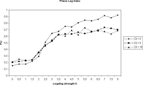
Results for the Kuramoto model are summarized in Figures 1, 2, 3. Figure 1 shows the mean PC, averaged over all pairs of the 64 simulated EEG channels, as a function of coupling strength K and degree of overlap (number of oscillators contributing to each EEG channel). In the case of no overlap, PC stayed at relatively low levels for K lower than 2. From K = 2 onwards, there was a sudden and strong increase of PC, which leveled of for high values of K (recall that we used γ = 1, that is, K _crit = 2). This behavior of PC is in close agreement with the analytical results for the model, that is, the known bifurcation to at the critical level of K = K _crit = 2. When the overlap between EEG channels was modified from 0 to 8 clear changes in PC were found. First, the entire curve was shifted toward a higher level for all values of K. Second, the relative increase in PC started at lower values than the analytically expected value of K _crit = 2. Increasing the level of overlap between EEG channels from 8 to 16 showed an upward displacement of the curve, but only for values of K < 2.5. The relative increase of PC started at even lower values of K. Thus, while PC was sensitive to true changes in the connection strength K, it was also quite sensitive to spurious influences of common sources, which changed both the absolute values as well as the qualitative behavior of PC as a function of K.

Figure 1.

Mean phase coherence (PC, averaged over all possible pairs of 64 modeled EEG channels) as a function of coupling strength K in the Kuramoto model with 64 oscillators as a function of overlap between subsequent EEG channels (CS: common sources, ranging from 0 to 16). All results are the average to 10 trials. The first 5,000 samples of each trial were ignored. Epoch length for each trial was 4,096 samples. Mean frequency of the oscillators in the model was 10 Hz, the width of the Lorentz distribution γ = 1. Sample frequency was 500 Hz. These parameters yield a critical value of K _crit = 2.

Figure 2.

Mean phase lag index (PLI, averaged over all possible pairs of 64 modeled EEG channels) as a function of coupling strength K in the Kuramoto model. Parameters are identical with Figure 1.

Figure 3.

Mean absolute value of the imaginary part of coherency (IC, averaged over all possible pairs of 64 modeled EEG channels) as a function of coupling strength K in the Kuramoto model. For parameters see Figure 1.

The results for PLI are depicted in Figure 2. In the ideal case without common sources, PLI showed low values for K < K _crit, and increasing values for higher K as expected from theory. Compared to PC, however, PLI started to increase at somewhat lower values of K. Adding the influence of common sources increased PLI values slightly for K < 2.5 and decreased the PLI values for K > 2.5. For very high values of K, PLI underestimated the true level of coupling. There was no clear difference between an overlap of 8 or 16 oscillators. Thus, PLI also showed the expected increase as a function of K but compared with PC, it was less sensitive to the spurious influence of common sources.

Finally, the results for IC are shown in Figure 3. In the absence of volume conduction, IC started to increase for K > K _crit, but never reached values much higher than IC = 0.2 even for very high coupling strength K (note that the upper bound for IC is 1). That is, IC systematically underestimated the true coupling strength in the model. For increasing effects of volume conduction, IC increased for K≤ 2.5 and decreased for K > 2.5. Hence, the effects of simulated volume conduction further compromised the modest sensitivity of IC to increase in coupling strength.

EEG and MEG Recording

Absence EEG

The transition between inter‐ictal to ictal EEG is shown in Figure 4. The results for the absence EEG are given in Figures 5, 6, 7. Figure 5 shows the mean PC averaged over all possible electrode pairs for each of the epochs and for various different montages. By and large PC stayed roughly constant at a baseline level during the first 5 nonseizure epochs. After that, we found a sudden increase in PC in epoch 6 and 7, which contained the generalized spike‐and‐wave discharges. In the final epochs (8–11), PC decreased to the baseline level.

Figure 4.

Detail of EEG recording with absence seizure consisting of ∼3 Hz generalized spike‐and‐slow wave discharges. Average reference, filter settings: high pass 0.5 Hz and low pass 48 Hz. Vertical blue bars indicate 1 s intervals. [Color figure can be viewed in the online issue, which is available at www.interscience.wiley.com.]

Figure 5.

Mean PC (averaged over all pairs of 21 channels) for different montages (average, source, mastoids, bipolar, and Cz). Each epoch has a length of 4,096 samples (8.18 s). Epoch no. 6 and 7 correspond to the seizure.

Figure 6.

Mean PLI (averaged over all pairs of 21 channels) for different montages (average, source, mastoids, bipolar, and Cz). Each epoch has a length of 4,096 samples (8.18 s). Epoch no. 6 and 7 correspond to the seizure.

Figure 7.

Mean IC (averaged over all pairs of 21 channels) for different montages (average, source, mastoids, bipolar, and Cz). Each epoch has a length of 4,096 samples (8.18 s). Epoch no. 6 and 7 correspond to the seizure.

As can be seen in Figure 5, the montages had quite an influence on PC values. The lowest values were found for the source (local average) derivation. Slightly higher values were obtained for the bipolar derivation. Values of PC were even higher for average reference and the linked ears derivation. There the linked ears derivation showed the strongest relative increase by a factor of 2.5 during the seizure as compared to baseline. The highest values during baseline as well as the lowest values during the seizure were obtained with the Cz reference; relative increase was less than a factor of 1.5. Overall, the type of reference strongly influenced the absolute values of PC as well as the relative increase during the seizure.

The results for PLI are depicted in Figure 6. During the five preseizure epochs, PLI stayed more or less constant at a low level slightly above 0.1. During the seizure epochs 6 and 7, a clear increase could be found. This increase was followed by an immediate decrease in epochs 8–11. During the preseizure epochs, PLI values were hardly influenced by different derivations. During the seizure differences did emerge: PLI values were low for the Cz derivation, intermediate for the average reference and the linked ears reference, and highest for the bipolar and source derivation. The relative increase in PLI during the seizure was roughly a factor of 3 for the worst reference (Cz) and a factor of 5 for the best (source). In the early post seizure epochs 8 and 9, PLI values were still higher than in the pre‐seizure epochs, especially for the average reference and the linked ears reference. Overall, PLI undoubtedly showed increases during the seizure epochs and was less influenced by the different montages than PC, although differences could still be seen during the seizure. Expressed as relative increase (synchronization during seizure compared to baseline) PLI performed better than PC for all montages.

The results for IC are shown in Figure 7. For the preseizure epochs, the IC of the different montages fluctuated around 0.04. After that, we found a clear increase during the seizures epochs (6–7), which was followed by a gradual decrease in the postictal epochs. The different montages had only a small effect on IC for the pre‐ and post‐ictal epochs, but during the seizure there were differences: IC was relatively low for Cz (relative increase factor 2) and high for the bipolar montage (relative increase factor 3.5). The other montages showed intermediate values. Thus, for detecting a relative increase in synchronization from pre seizure to seizure epochs, IC performed better than PC and only slightly worse than the PLI.

Alzheimer and control EEG

Results of the synchronization analysis of the Alzheimer and control EEGs are shown in Figures 8, 9, 10. Average PC in the beta band was lower in Alzheimer patients than in controls (P = 0.023; Fig. 8). Analyses of sub averages for long and short distances and intra/interhemispheric electrode pairs did not reveal significant differences, although there was an almost significant (P = 0.054) decrease in short distance intra hemispheric PC in the Alzheimer group. Results for PLI are given in Figure 9. The average PLI in the beta band was significantly lower in the Alzheimer group compared with controls (P = 0.009). Further analysis revealed that PLI values for both short (P = 0.032) and long distance (P = 0.016) intrahemispheric electrode pairs were lower in the Alzheimer group. Results for IC are shown in Figure 10. The average IC was significantly lower in Alzheimer patients (P = 0.002). Further analysis showed that this was due to a significantly lower IC in Alzheimer patients for short intrahemispheric distances (P = 0.005) and long interhemispheric distances (P = 0.013). Overall, PLI and IC were better in distinguishing between Alzheimer patients and controls than PC. Also, PC showed a clear drop from short to long distances, which was less pronounced for IC and virtually absent for PLI.

Figure 8.

Mean PC for 15 subjects with Alzheimer's disease and 13 control subjects with subjective memory complaints. Error bars indicate standard deviations. Results are the average of four epochs (average reference, epoch length 4,096 samples, 21 channels, digitally filtered between 13 and 30 Hz, sample frequency 500 Hz). Total: average of all pairs of 21 channels; intra_s: average of all short, intrahemispheric electrode pairs; intra_l: average of all long intrahemispheric electrode pairs; inter_s: average of all short interhemispheric electrode pairs; inter_l: average of all long interhemispheric electrode pairs. Details of the specific electrode pairs making up the four sub averages can be found in the methods section.

Figure 9.

Mean PLI for 15 subjects with Alzheimer's disease and 13 control subjects with subjective memory complaints; cf. Figure 8.

Figure 10.

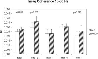
Mean IC for 15 subjects with Alzheimer's disease and 13 control subjects with subjective memory complaints; cf. Figure 8.

MEG data

MEG data of two healthy subjects were analyzed to illustrate the influence of volume conduction on spatial patterns of functional connectivity. Results are summarized in Figure 11. In both subjects, the highest values for the 8–13 Hz PC in the no‐task, eyes‐closed state showed a characteristic pattern with a clear predominance of small distances and a virtual absence of long distances. In contrast, the other measures (PLI and IC) displayed a different pattern. For subject A (upper row), PLI showed the strongest correlations between a cluster of channels above right temporal/occipital areas and a number of strong left central to right temporal/occipital correlations. The IC had a similar spatial pattern as well as a number of left and right fronto temporal correlations. For subject B (lower row), PLI showed strong correlations radiating from occipital regions to temporal and frontal regions as well as left/right correlations over the posterior areas. The IC showed a somewhat similar pattern but with more relatively short distance correlations over the right temporal area.

Figure 11.

Illustration of the spatial distribution of the strongest correlations between pairs of MEG channels using either phase coherence (PC, left column), the phase lag index (PLI, middle column) or the imaginary part of coherency (IC, right column). Data are collected from two different healthy subjects (upper row and lower row). In all maps, only correlations above threshold are displayed. The threshold was chosen such that sufficiently many connections were visible to allow for a proper evaluation of the spatial pattern of supra threshold connections. Eyes closed, no task MEG (sample frequency 312.5 Hz; filter settings: 8–13 Hz). Epoch length 4,096 samples (13.083 s).

DISCUSSION

We have introduced the PLI as a novel measure of phase synchronization exploiting the asymmetry of the distribution of instantaneous phase differences between two signals. In numerical simulations of the Kuramoto model, PLI increased as a function of coupling strength contrasting IC and was less sensitive to volume conduction than PC. In EEG absence data, PC was more sensitive to montage effects than both PLI and IC. PLI and IC performed better in detecting loss of EEG beta band connectivity in Alzheimer patients compared with controls. Finally, the spatial pattern of MEG alpha band connectivity based upon PC was different form the patterns based upon either PLI or IC, which were quite similar to each other.

We used the Kuramoto model of globally coupled oscillators to study the effects of changes in true synchronization and ‘volume conduction’ on PC, PLI, and IC for two major reasons: (i) the oscillators may present a natural model for oscillatory EEG or MEG activity; (ii) the behavior of the model is very well studied and, e.g., the onset of synchronization as a function of coupling strength is exactly known [Strogatz, 2000]. We modeled ‘volume conduction’ quite simplistically by allowing for more than a single oscillator to contribute to each simulated EEG channel. While this construction strongly exaggerated effects of volume conduction, it allowed for testing the behavior of the various measures under extreme conditions. Notice that modeling realistic sources in a volume conductor is beyond the scope of the present paper. Also, use of a more biologically inspired model of the EEG would have the disadvantage that in such models the exact relation between changes in coupling strength and synchronization is not analytically accessible.

Our model simulations showed that, as expected, both PC and PLI responded to increases in the coupling strength in the form of a sudden increase at the bifurcation point, K = K _crit. While this result for PC appears obvious, it underlines the PLI's capacities, although PLI is constructed to just detect non zero phase lag coupling. That is, PLI is able to detect synchronization in the Kuramoto model with moderate coupling strength. With very high values of K, the mean phase difference between all the oscillators vanishes, which might explain why the PLI does not reach a value of one. Compared with PLI, IC performed much worse, probably because it simply reflects the small value of the mean phase difference even for relatively small values of K. The model showed that PC is strongly influenced by the simulated volume conduction effects, although it still increases with increases in coupling strength. This suggests that absolute values of PC cannot be interpreted in the context of (unknown) influences of volume conduction, while changes in PC between experimental conditions and/or groups could still reflect changes in coupling. However, if the volume conduction effects also change as a function of condition or group, then this conclusion is no longer valid. Although PLI is not immune to the volume conduction, these effects are clearly smaller than for PC, especially for moderately high values of K. This readily suggests that for all practical purposes PLI might be a more reliable measure of “true” synchronization than PC. The IC was clearly influenced by the simulated volume conduction in the model, especially for high values of K. This influence might be caused by a (relative) decrease of coherency's imaginary component in the case of a simultaneous increase in the value of the real component—the latter will increase if the zero phase lag coupling in the data increases. Thus, while the existence of an imaginary component cannot be explained by volume conduction, its value can still be influenced by it.

While being useful for studying certain features of coupling measures under well‐controlled circumstances, modeling cannot predict the extent to which these measures will perform with experimental data. To illustrate their performance, we studied the paradigmatic case of strongly increased synchronization (EEG in absence seizure) and an example of a fairly subtle decrease of synchronization and spatial connectivity patterns in MEG. In the absence data, all three measures showed an increase during the seizure. Note that increased synchronization during absence seizures is a well‐known phenomenon, which should be reproduced by any useful measure of synchronization [Amor et al., 2005; Mormann et al., 2000]. For EEG, however, different montages and active reference electrodes may strongly influence the outcome of estimated synchronization between the channels [Guevara et al., 2005; Lachaux et al., 1999; Nunez et al., 1997].

The influence of montage was quite clear for the PC, where both preictal, ictal, and postictal values were affected. The PC values were lowest for the source derivation and highest for the Cz reference. The source derivation performed best in terms of the relative increase during the seizure. These results agree with studies on coherence by Nunez and coworker [1997]. Note that Mima et al. [2000] already suggested the relative superiority of the source derivation for estimating true coupling. In contrast to PC, both PLI and IC were less sensitive to influences of montage. In the pre‐ and post‐ictal phases, montage had almost no effect but during the seizure we found differences. There, the source montage performed best, especially for PLI showing a relative increase when compared with preictal levels by a factor of 5 (compared with a maximum increase by a factor of 3.5 for IC). Thus, even with PLI and IC, the choice of montage still has an impact but performance in terms of detecting changes in levels of synchronization is clearly increased when compared with PC.

The Alzheimer data set was used to study the sensitivity of the three measures in detecting subtle changes in beta band coupling. Such changes were already demonstrated for this data set in another study [Stam et al., 2006]. The PC showed a moderately significant overall loss of beta band synchronization but could not further differentiate this group effect in long/short distance of intra‐/inter‐hemispheric components. Of interest, PC was consistently higher for short distances implying volume conduction effects. In contrast, both PLI and IC showed more significant group differences and revealed more details of the types of connections contributing to this group difference. Also, especially for PLI, there was almost no difference between short and long distances, which suggests a diminished influence of volume conduction. An important conclusion that can be drawn from this data set is that even in the noisy beta band, which shows only weak coupling and small group differences, it is possible to detect non zero phase lag synchronization. The existence of nonzero phase lag coupling has already been shown at the neuronal level [Roelfsema et al., 1997] and in intracranial recordings [Tallon‐Baudry et al., 2001]. While zero phase lag coupling could be due to both volume conduction/active reference electrodes and true coupling, nonzero phase lag coupling is more likely to reflect true coupling of underlying sources. Thus, the existence of this type of coupling in resting state brain activity and the fact that it is changed in a neurological disorder are of considerable theoretical interest. In the study of Thatcher et al. [2005], coupling with a small phase lag between frontal EEG channels was the EEG measure most strongly correlated to intelligence.

Finally, we studied whether volume conduction effects in MEG might reflect the spatial patterns of estimated functional connectivity. Recently, Langheim et al. [2006] described such patterns in some detail. The pattern of alpha band connectivity based upon PC, displayed by showing sensor pairs with a PC above a certain threshold as a two‐dimensional graph, showed some similarity to the patterns in the paper by Langheim and coworkers. However, both PLI and IC showed a completely different spatial pattern. Remarkably, PLI and IC patterns were quite similar to each other in both subjects. The comparison between the PC pattern on the one hand and the PLI and IC patterns on the other hand clearly revealed that the PC pattern was dominated by local connections between adjacent sensors. Such local connections were absent in PLI and IC patterns, which were dominated by long distance interactions. This result suggests that, for MEG, PC estimates for nearby channels were strongly influenced by volume conduction and that this influence was diminished in the case of PLI and IC.

Quantifying (the strength of) interaction by PLI, and similarly by IC, one certainly accepts the risk to miss linear but functionally meaningful interactions, which, in principle, might be expressed in near zero phase coherence. Here, we would like to stress that this potential omission is deliberate and, while realizing that the remaining information might be incomplete, PLI (and IC) are clearly free of any artefacts of volume conductions. We believe that the latter are the by far most frequent cause for misinterpretation of more general measures of interaction. We must admit, however, that the obvious question “How much do we miss?” can yet not be answered as it, above all, depends on the specific nature of the system under study.2

Nolte and colleagues [2004] have shown that a nonvanishing imaginary component of coherency cannot be explained by volume conduction. Such a rigorous statement yet awaits to be proven for PLI, although the correlation structure of the analytical signal (which forms the basis for our phase definition) does indicate certain symmetries of the corresponding phase distribution (see Appendix B). Furthermore, Guevara and coworkers recently expressed their concerns about phase synchronization with lags [Guevara et al., 2005]. Lachaux et al. stated that “Another common assumption is that the phase difference between electrodes should be zero in case of conduction synchrony. This is usually false …” [Lachaux et al., 2005: page 202]. Thus, the fact that PLI is only sensitive to phase synchronization with a nonzero phase lag is no guarantee that it will not be affected by volume conduction. Our results suggest, however, that it may be significantly less sensitive to such effects than the commonly used PC. Also, in contrast to IC, PLI is a fairly simple measure of phase synchronization that is closely related to estimates based on the phase distribution's (Shannon) entropy [e.g., Tass et al., 1998]. We have shown that PLI performs quite well both in a model as well as in different types of empirical data. For the latter, the PLI and IC performed equally well and were superior to PC. In conclusion, we suggest using one of these measures when studying functional connectivity with EEG or MEG, especially when this analysis is based on signal space.

Appendix A: Imaginary Part of Coherency

To compute the frequency dependent correlations between different encephalographic channels, we assume that {s_k(f)} is a finite set of statistically independent common sources yielding signals x _m at channel m in the form of a linear combination like

(A1)

Statistical independence implies the sources' cross‐spectral densities—for the sake of legibility, we here omit any normalization and use the cross‐spectral density rather than coherency, cf. Eq. (7)—have the form

(A2)

in which δ_{kk ′} denotes the Kronecker‐delta. By the use of Eq. (A2) one can readily conclude that the cross‐spectral density S _mn between x _m and x _n is real since we find

(3)

In words, a set of uncorrelated sources s_k (∼volume conduction), each of which being recorded at channel m with weighting factor a _mk, only causes a real‐valued coherency (the cross‐phase spectrum vanishes for phases other than 0 or ±π, dependent on the sign of S _mn).

By the same reasoning, but being a bit more realistic, we pick two distinct sources, s_p and s_q and assume that those are (nonlinearly) correlated. Thus, we replace Eq. (A2) by

(A4)

with p ≠ q and . Using Eq. (A4) yields for the cross‐spectral density between x _m and x _n

(A5)

Hence, volume conduction may alter the coherency, which is originally caused by correlated sources s_p and s_q, only by a shift along the real axis: the source s_k do not intermingle along some nontrivial direction, although here two of them are already correlated. That is, if is real‐valued (i.e., has a mean phase at 0 or ±π), then an additional, arbitrary number of uncorrelated sources that “infiltrate” the recording channels via volume conduction cannot rotate coherency toward an imaginary direction. Put differently, a phase distribution that does not peak around 0 or ±π cannot be caused by volume conduction.

Appendix B: Correlation of Analytic Signals

To compare the above results with the numerical estimates based on simulation and empirical data, we use the same line of reasoning but stay in the time‐domain rather than (Fourier‐) transforming to a frequency representation. Phase will then no longer be given by the cross‐spectrum in the Fourier domain but via the Hilbert phase. In detail, we take

(B1)

for which we construct the analytical signal using the Hilbert transform (i.e. the convolution with t ⁻¹)

(B2)

the integral represents the Cauchy principal value (PV), see also Eq. (3). This convolution forms the imaginary part of the analytical signals that we write as

(B3)

where y_k are the analytical signals corresponding to sources s_k (for the equality on the right‐hand side, we used the linearity of Eq. (B1) and dissociativity of the convolution).

For the sake of simplicity, we always assume that all sources have vanishing mean, i.e. . Further, we assume that the sources are uncorrelated3 by means of

(B4)

α _k denotes the autocorrelation function of source s_k. This readily yields vanishing cross‐correlations for the corresponding analytical signals, that is, we find

(B5)

Notice that we write the conjugate complex in brackets to leave the definition of the correlation function of complex signals open, at least for the time being. Notice also that we are primarily interested in the instantaneous correlation, that is, at the end of the day we will compute the limit Δ → 0. Hence, we need to compute the autocorrelation of the analytic signal, for which we obtain (for the sake of legibility we dropped the PV‐notation in front of the integrals)

(B6)

The first term on the right‐hand side of Eq. (B6) is finite, while the last ones cancel each other as

(B7)

which, without the conjugate complex form (‘+’), trivially yields zero for the last terms in Eq. (B6) and. For the conjugate complex form (‘−’), one can exploit the symmetry of the autocorrelation function by means of when taking the limit Δ → 0 (see above). For the middle term in Eq. (B6) we find

(B8)

As announced, we evaluate the limit for Δ → 0, exploit the symmetry of α_k(τ), and, of course, we assume the integrability of the autocorrelation function α_k(τ) divided by τ that results in

(B9)

In summary, we have

(B10)

so that the cross‐correlation between analytical signals at channels m and n becomes

(B11)

Importantly, Eq. (B11) yields only real values so that the phase of the cross‐correlation is always 0 or ±π in agreement with Eq. (A3).

The next step is to allow for two sources to be nontrivially correlated and to look for potential effects of the present independent sources. In line with Eq. (A4), we assume that

(B12)

This causes the autocorrelation as summarized in Eq. (B9) but also generates additional cross‐terms of the form

(B13)

Consequently, Eq. (B11) can be replaced by

(B14)

EQN>

In words, conform with Eq. (A5), volume conduction may change the (zero‐lag or instantaneous) correlation between two analytical signals z _m and z _n at channels m and n, which is originally caused by two nontrivially correlated sources s_p and s_q, only by a shift along the real axis.

In fact, this correlation structure does not imply that a symmetric distribution of the corresponding relative Hilbert phase (i.e. peaking at 0 or ±π) necessarily stays symmetric in the presence of common sources, as this also depends on the corresponding Hilbert amplitudes, the sources independence renders a correlated impact of amplitudes unlikely. Put differently, it is quite likely that the uncorrelatedness of sources (or even their complete statistical independence) causes an invariance of the phase distributions symmetry against the presence of common sources. A rigorous proof for this, admittedly somewhat hand waving, argument, is yet to be found.

REFERENCES

- Amor F,Rudrauf D,Navarro V,N'diaye K,Garnero L,Martinerie J,Le van Quyen M ( 2005): Imaging brain synchrony at high spatio‐temporal resolution: Application to MEG signals during absence seizures. Signal Process 85: 2101–2111. [Google Scholar]
- Breakspear M ( 2002): Nonlinear phase desynchronization in human electroencephalographic data. Hum Brain Mapp 15: 175–198. [DOI] [PMC free article] [PubMed] [Google Scholar]
- Breakspear M,Terry JR ( 2002): Nonlinear interdependence in neural systems: Motivation, theory, and relevance. Int J Neurosci 112: 1263–1284. [DOI] [PubMed] [Google Scholar]
- Breakspear M,Williams LM,Stam CJ ( 2004): A novel method for the topographic analysis of neural activity reveals formation and dissolution of ‘dynamic cell assemblies’. J Comput Neurosci 16: 49–68. [DOI] [PubMed] [Google Scholar]
- Barry RJ,Clarke AR,McCarthy R,Selikowitz M ( 2005): Adjusting EEG coherence for inter‐electrode distance effects: An exploration in normal children. Int J Psychophysiol 55: 313–321. [DOI] [PubMed] [Google Scholar]
- Burns A ( 2004): Fourier‐, Hilbert‐ and wavelet‐based signal analysis: Are they really different approaches? J Neurosci Methods 137: 321–332. [DOI] [PubMed] [Google Scholar]
- David O,Garnero L,Cosmelli D,Varela FJ ( 2002): Estimation of neural dynamics from MEG/EEG cortical current density maps: Application to the reconstruction of large‐scale cortical synchrony. IEEE Trans Biomed Eng 49: 975–987. [DOI] [PubMed] [Google Scholar]
- Fingelkurts AA,Fingelkurts AA,Kahkonen S ( 2005): Functional connectivity in the brain—is it a elusive concept? Neurosci Biobehav Rev 28: 827–836. [DOI] [PubMed] [Google Scholar]
- Fries P ( 2005): A mechanism for cognitive dynamics: Neuronal communication through neuronal coherence. Trends Cogn Neurosci 9: 474–480. [DOI] [PubMed] [Google Scholar]
- Friston KJ ( 2001): Brain function, nonlinear coupling, and neuronal transients. Neuroscientist 7: 406–418. [DOI] [PubMed] [Google Scholar]
- Friston KJ ( 2002): Functional integration and inference in the brain. Prog Neurobiol 68: 113–143. [DOI] [PubMed] [Google Scholar]
- Gross J,Kujala J,Hamalainen M,Timmermann L,Schnitzler A,Salmelin R ( 2001): Dynamic imaging of coherent sources: Studying neural interactions in the human brain. Proc Natl Acad Sci USA 98: 694–699. [DOI] [PMC free article] [PubMed] [Google Scholar]
- Guevara R,Velazguez JLP,Nenadovic V,Wennberg R,Senjanovic G,Dominguez LG ( 2005): Phase synchronization measurements using electroencephalographic recordings. What can we really say about neuronal synchrony? Neuroinformatics 4: 301–314. [DOI] [PubMed] [Google Scholar]
- Hadjipapas A,Hillebrand A,Holliday IE,Singh K,Barnes G ( 2005): Assessing interactions of linear and nonlinear neuronal sources using MEG beamformers: A proof of concept. Clin Neurophysiol 116: 1300–1313. [DOI] [PubMed] [Google Scholar]
- Kiss IZ,Zhar Y,Hudson JL ( 2002): Emerging coherence in a population of chemical oscillators. Science 296: 1676–1678. [DOI] [PubMed] [Google Scholar]
- Kuramoto Y ( 1975): Self‐entrainment of a population of coupled nonlinear oscillators In: Int. Symp. on Math. Prob. in Theor. Physics H. Araki, ed., Springer‐Verlag, New York, Lecture notes in physics 39, 420–422. [Google Scholar]
- Lachaux J‐P,Rodriguez E,Martinerie J,Varela FJ ( 1999): Measuring phase synchrony in brain signals. Hum Brain Mapp 8: 194–208. [DOI] [PMC free article] [PubMed] [Google Scholar]
- Langheim FJP,Leuthold AC,Georgopoulos AP ( 2006): Synchronous dynamic brain networks revealed by magnetoencephalography. Proc Natl Acad Sci USA 103: 455–459. [DOI] [PMC free article] [PubMed] [Google Scholar]
- Lee L,Harrison LM,Mechelli A ( 2003): A report of the functional connectivity workshop, Dusseldorf 2002. Neuroimage 19: 457–465. [DOI] [PubMed] [Google Scholar]
- Lehmann D,Faber PL,Gianotti LRR,Kochi K,Pascual‐Marqui RD ( 2006): Coherence and phase locking in the scalp EEG and between LORETA model sources, and microstates as putative mechanisms of brain temporo‐spatial functional organization. JPhysiol 99: 29–36. [DOI] [PubMed] [Google Scholar]
- Le van Quyen M ( 2003): Disentangling the dynamic core: A research program for a neurodynamics at the large scale. Biol Res 36: 67–88. [DOI] [PubMed] [Google Scholar]
- Mardia KV ( 1972): Statistics of Directional Data. London: Academic Press. [Google Scholar]
- Mima T,Matsuoka T,Hallett M ( 2000): Functional coupling of human right and left cortical motor areas demonstrated with partial coherence analysis. Neurosci Lett 287: 93–96. [DOI] [PubMed] [Google Scholar]
- Mormann F,Lehnertz K,David P,Elger CE. ( 2000): Mean phase coherence as a measure for phase synchronization and its application to the EEG of epilepsy patients. Physica D 144: 358–369. [Google Scholar]
- Nolte G,Wheaton OBL,Mari Z,Vorbach S,Hallett M ( 2004): Identifying true brain interaction from Eeg data using the imaginary part of coherency. Clin Neurophysiol 115: 2292–2307. [DOI] [PubMed] [Google Scholar]
- Nunez PL,Srinivasan R,Westdorp AF,Wijesinghe RS,Tucker DM,Silberstein RB,Cadusch PJ ( 1997): EEG coherency. I. Statistics, reference electrode, volume conduction, Laplacians, cortical imaging, and interpretation at multiple scales. Electroencephalogr Clin Neurophysiol 103: 499–515. [DOI] [PubMed] [Google Scholar]
- Nunez PL,Silberstein RB,Shi Z,Carpenter MR,Srinivasan R,Tucker DM,Doran SM,Cadusch PJ,Wijesinghe RS ( 1999): EEG coherency. II. Experimental comparisons of multiple measures. Clin Neurophysiol 110: 469–486. [DOI] [PubMed] [Google Scholar]
- Pereda E,Quian Quiroga R,Bhattacharya J ( 2005): Nonlinear multivariate analysis of neurophysiological signals. Prog Neurobiol 77: 1–37. [DOI] [PubMed] [Google Scholar]
- Roelfsema PR,Engel AK,Konig P,Singer W ( 1997): Visuomotor integration is associated with zero time‐lag synchronization among cortical areas. Nature 385: 157–161. [DOI] [PubMed] [Google Scholar]
- Rosenblum MG,Pikovsky AS,Kurths J ( 1996): Phase synchronization of chaotic oscillators. Phys Rev Lett 76: 1804–1807. [DOI] [PubMed] [Google Scholar]
- Salvador R,Suckling J,Coleman MR,Pickard JD,Menon D,Bullmore E ( 2005): Neurophysiological architecture of functional magnetic resonance images of human brain. Cereb Cortex 15: 1332–1342. [DOI] [PubMed] [Google Scholar]
- Singer W ( 1999): Neuronal synchrony: A versatile code for the definition of relations? Neuron 24: 49–65. [DOI] [PubMed] [Google Scholar]
- Stam CJ ( 2005): Nonlinear dynamical analysis of EEG and MEG: Review of an emerging field. Clin Neurophysiol 116: 2266–2301. [DOI] [PubMed] [Google Scholar]
- Stam CJ ( 2006): Nonlinear Brain Dynamics. New York: Nova Science Publishers. [Google Scholar]
- Stam CJ,Jones BF,Nolte G,Breakspear M,Scheltens P ( 2007): Small world networks and functional connectivity in Alzheimer's disease. Cereb Cortex 17: 92–99. [Epub 2006, Feb. 1] [DOI] [PubMed] [Google Scholar]
- Strogatz SH ( 2000): From Kuramoto to Crawford: Exploring the onset of synchronization in populations of coupled oscillators. Physica D 143: 1–20. [Google Scholar]
- Strogatz SH ( 2001): Exploring complex networks. Nature 410: 268–276. [DOI] [PubMed] [Google Scholar]
- Tallon‐Baudry C,Betrand O,Fischer C ( 2001): Oscillatory synchrony between human extrastriate areas during visual short‐term memory maintenance. J Neurosci 21: 1–5. [DOI] [PMC free article] [PubMed] [Google Scholar]
- Tass P,Rosenblum MG,Weule J,Kurths J,Pikovsky A,Volkmann J,Schnitzler A,Freund H‐J ( 1998): Detection of n:m phase locking from noisy data: Application to magnetoencephalography. Phys Rev Lett 81: 3291–3294. [Google Scholar]
- Tass PA,Fieseler T,Dammers J,Dooolan K,Morosan P,Majtanik M,Boers F,Muren A,Zilles K,Fink GR ( 2003): Synchronization tomography: A method for three‐dimensional localization of phase synchronized neuronal populations in the human brain using magnetoencephalography. Phys Rev Lett 90: 088101. [DOI] [PubMed] [Google Scholar]
- Tononi G,Edelman GM,Sporns O ( 1998): Complexity and coherency: Integrating information in the brain. Trends Cogn Sci 2: 474–484. [DOI] [PubMed] [Google Scholar]
- Varela F,Lachaux J‐P,Rodriguez E,Martinerie J ( 2001): The brainweb: Phase synchronization and large‐scale integration. Nat Rev Neurosci 2: 229–239. [DOI] [PubMed] [Google Scholar]
- Wheaton LA,Nolte G,Bohlhalter S,Fridman E,Hallett M ( 2005): Synchronization of parietal and premotor areas during preparation and execution of praxis hand movements. Clin Neurophysiol 116: 1382–1390. [DOI] [PubMed] [Google Scholar]