Bayesian inverse analysis of neuromagnetic data using cortically constrained multiple dipoles

INTRODUCTION

Magnetoencephalography (MEG) provides millisecond‐scale measurements of the extracranial magnetic fields generated by neural activity in the human brain [Hämäläinen et al.,1993]. The accurate timing information is crucial both in clinical applications and also in cognitive neuroscience research. However, the localization of the underlying neural generators requires the solving of the electromagnetic inverse problem, which is ill‐posed and does not have a unique solution [Sarvas,1987].

The neuromagnetic inverse problem is often constrained by utilizing the equivalent current dipole (ECD) model [Baillet et al.,2001; Mosher et al.,1992]. In the ECD model, one assumes that the neural source can be truthfully represented by a set of current dipoles. Even though dipole fitting in many cases is an adequate method, it is important to notice that the actual cortical activation pattern that produces the fields visible to MEG is assumed to be elicited by synchronous postsynaptic potentials of a large number of cortical pyramidal neurons [Dale and Sereno,1993; Okada et al.,1997] and therefore the activation might extend over few square centimeters of gray matter and the use of dipoles may no longer be plausible. Also, ECD fitting in its basic form requires both expertise from the user and some prior knowledge of the possible number and locations of the current dipoles.

Other popular methods for tackling the electromagnetic inverse problem include several extended or distributed source current estimates, such as the ℓ² [Hämäläinen and Ilmoniemi,1984; Hauk,2004] and ℓ¹ minimum‐norm [Matsuura and Okabe,1995; Uutela et al.,1999] estimates, MNE and MCE, respectively. The minimum‐norm estimates have been further elaborated by using anatomical magnetic resonance imaging (MRI)‐based cortical constraints, in which the orientation of the current source in each distributed cortical location is restricted to be perpendicular [Dale and Sereno,1993; with ℓ²] or almost perpendicular [Lin et al.,2006; with ℓ¹ and ℓ²] to the surface normal. Other examples of improving the MNE are, for instance, noise sensitivity normalization [Dale et al.,2000], depth weighting [Köhler et al.,1996], and constraining the solutions with functional magnetic resonance imaging (fMRI) data [Liu et al.,1998].

During the past 10 years, Bayesian formulation of the electromagnetic inverse problem [Auranen et al.,2005; Baillet and Garnero,1997; Friston et al.,2002a,b; Phillips et al.,1997; Schmidt et al.,1999] has caught on with the MEG research community. The fast development of computing power has enabled the use of Markov chain Monte Carlo (MCMC)‐methods in obtaining the solution to the inverse problem using various different procedures ranging from basic Metropolis sampler to reversible jump MCMC (RJMCMC) and parallel tempering (PT) algorithms [Bertrand et al.,2001; Kincses et al.,2003; Schmidt et al.,1999].

Recently, Jun et al. [2005] proposed a Bayesian inference technique for multiple dipole analysis of MEG data having a full spatiotemporal sensor space noise covariance structure. They show, for example, that their method is faster than the one utilizing extended region model [Schmidt et al.,2000], and that it does not require prior determination of the number of dipoles. Here, we have implemented a similar Bayesian model with several technical modifications. (i) Instead of a spherical forward model and continuous three‐dimensional source space grid, we utilize a more realistic forward model based on the subject's individual anatomy and (ii) cortical constraints so that the location and orientation of the sources were restricted to be on the white–gray matter boundary and perpendicular to the cortical mantle, correspondingly. The FreeSurfer software we employed for determining the cortical geometry allows inflation of the cortical surface into a sphere thus giving (iii) a compact parametrization of the source space grid point locations in spherical coordinates [Fischl et al.,1999]. This continuous and bounded parameter space makes it possible to use adaptive method of slice sampling [Neal,2003], which should in principle switch well between different modes of the sampled posterior distribution. The sampling of number of dipoles and random state jumps were performed with RJMCMC and Metropolis algorithms. As all the MEG sensors are not independent, we (iv) used singular value decomposition (SVD) to reduce the number of linearly independent measurement combinations with minimal loss of information, leading to a slightly smoother posterior distribution (i.e., regularization) and tremendous acceleration of computations. The method was tested with both empirical and realistically simulated MEG data for simple audiovisual sensory stimulation, providing a challenging and interesting exploratory case for such an inverse model.

We show that despite some problems related to the multimodality of the posterior and poor switching of the modes during sampling, our model performs well with both realistically simulated and empirical data, localizing the dipoles to a physiologically feasible locations on the white–gray matter boundary. Our findings also suggest that with cortical constraints, a good data fit even to simple audiovisual data requires more than two or three dipolar sources, causing difficulties to our model as it can handle only relatively small number of sources well. Finally, we discuss the possibility to combine two methods, the variational hierarchical MNE [Nummenmaa et al., 2006; Sato et al.,2004)] and our local dipole sampler, for producing a hybrid method possibly capable of more precise localization and characterization of the complicated posterior distribution.

MATERIALS AND METHODS

The Bayesian Approach

In Bayesian formalism [for a review on Bayesian methods and data analysis see, Bernardo and Smith,1994; Gelman et al.,2003], the model parameters Θ and observables are conditioned with a set of modeling assumptions made by the analyst and together they set up a joint probability model P(,Θ|). In the analysis, the posterior probability of the model parameters P(Θ|,) is given by the joint probability of the model parameters and data, divided by the evidence P(|) of the model, which can be omitted with fixed data and modeling assumptions. According to Bayes' theorem, the joint posterior is proportional to the product of the likelihood term of the data P(|Θ,) and parameter prior term P(Θ|):

(1)

The full posterior probability distribution of the parameters is typically very difficult to handle due to the high dimension of the parameter space and usually it is convenient to only compute some marginal densities or posterior expectations of some parameters. However, the high‐dimensional integrals involved may not be analytically solvable and some sophisticated computational methods are required. Often, MCMC methods [Gilks et al.,1996; Robert and Casella,2004] are used to represent the posterior (1) numerically.

Source Space and Forward Model

We assume that the neural source underlying the MEG data can be accounted for with current dipoles located on the white–gray matter boundary and oriented normal to the cortical surface. The source space was reconstructed from 3‐D T1‐weighted high‐resolution MR images (recorded at Department of Radiology, Helsinki University Central Hospital, Finland; Siemens 1.5 T device) using the FreeSurfer software [Dale et al.,1999; Fischl et al.,1999] and transferred into MATLAB‐environment for further processing. We created four different discretizations of the source space consisting of 16,000, 8,000, 4,000, and 3,000 points having an average grid point separation of 3.8, 5.4, 7.6, and 8.8 mm, respectively. A denser grid was used for the data simulations and coarser ones for the inverse analyses. This way, we avoid the most common crime in inverse estimation, i.e., the use of the same discretization both for creating the simulated data and in the inverse solution algorithm. To investigate the model sensitivity to the accuracy of the cortical constraints, we performed the inverse analysis with two different grid discretizations.

In the forward calculations, we employed a single‐layer boundary element model (BEM), assuming the skull to be a perfect insulator and the cranial volume to have a homogeneous and isotropic electrical conductivity. This is feasible in many cases of MEG source estimation [see, e.g., Hämäläinen and Sarvas,1989; Mosher et al.,1999]. The MEG sensor geometry is that of the Vectorview system (Elekta‐Neuromag Oy, Helsinki, Finland) in which 306 sensors are arranged in 102 locations (two sets of orthogonal gradiometers and one set of magnetometers in triplets). In the present model, we used only the gradiometer measurements (extremely noisy channels not included) to reduce the computational burden.

Model Components

Our model description is rather similar to that of Jun et al. [2005] excluding the differences due to the use of cortical constraints, spherical parametrization of dipole locations, and the SVD‐based speed‐up and regularization strategy. In the following, we use the same symbols as Jun et al. [2005] where applicable to facilitate the comparison of these two different implementations.

Parametrization of dipole locations

The two‐dimensional discretized cortex surface, represented by three‐dimensional Cartesian coordinates x, y, and z, is parametrizable with two continuous variables utilizing the spherical coordinates [Fischl et al.,1999], each hemisphere corresponding to a separate sphere. The coordinate transformation from spherical to Cartesian coordinates is [Råde and Westergren,1998]:

(2)

where r is the arbitrary radius of the sphere and the spherical angle coordinates are θ = [0,…,π] and ϕ = [0,…,2π]. The source space is naturally discretized; so in the above transformation, each source space grid point on one hemisphere is represented by a small patch on the surface of the corresponding sphere.

The likelihood

Assuming zero‐mean L‐dimensional normal distribution for noise, we can write the likelihood for the measurements as:

(3)

where parameters {θ,ϕ}_i and hs_i are N‐dimensional vectors containing the location of the ith, i = [1,…,N], dipole on either the left or the right hemisphere using spherical angle coordinates, B is T × L‐dimensional matrix containing the measurements, J _N is T × N‐dimensional matrix comprising the current time course vectors of N dipoles, A _N is N × L‐dimensional part of the whole gain matrix A containing only rows corresponding to the locations {θ,ϕ}_i of N dipoles, and C (LT × LT) is the noise covariance matrix. We assume that both dipole locations and the gain matrix A are constant over time T. The gain matrix is N ₀ × L‐dimensional, where L is the number of MEG sensors and N ₀ is the discretized locations of the source space, that is, possible locations for the N dipoles. Furthermore, T [in superscript of Eq. (3)] denotes matrix transpose, −1 [in superscript of Eq. (3)] matrix inversion, |·| the determinant, and vec(·) the Vec‐operator [Harville,1999] that transforms a matrix to a vector by stacking its columns.

The noise covariance prior

As the accurate estimation of the noise covariance is rather grievous, it is reasonable to model it as uncertain. To make the marginalization procedure tractable, we choose the kth inverted Wishart distribution [Jun et al.,2005] as a conjugate prior for C.

(4)

where

Tr(·) denotes matrix trace, Γ(·) the Euler Gamma function, k the degree of freedom (should be greater than 2r ₀), r ₀ = LT, and C ₀ is scale matrix parameter for the noise covariance. Note that even though Jun et al. [2005] claim that in this case the expectation E(C) with respect to Eq. (4) is C ₀, this is not the case unless, k = 3r ₀ + 2, which is seen by calculating [Gupta and Nagar,2000]. However, our model is not overly sensitive to the estimated noise covariance C ₀ due to the SVD strategy, so we used the value of k = 4r ₀, giving E(C) ≈ 0.5 × C ₀.

The prior for the current time courses

As like Jun et al. [2005], we also impose a Gaussian distribution prior to the current time courses. By assuming that the prior standard deviation of the current magnitude σ is the same for all N dipoles, we arrive at [Jun et al.,2005, for calculations]:

(5)

where C _cu is a T × T‐dimensional temporal correlation matrix. C _cu is parametrized with β > 0, so that larger β produces stronger correlation

(6)

where f _s is the sampling rate of the measurements in Hertz. In our analyses, we assumed a temporal correlation of β = 5 ms, prior standard deviation of σ = 40 nAm, and downsampled measurement data with f _s = 150 Hz.

The prior for the dipole number and locations

The determinant of the Jacobian of the transformation (2) is after simple calculation found to be r ² sin(θ). Thus, in our model in which, instead of Cartesian coordinates, the sampling of dipole locations is done in spherical coordinates, we must take into account that the probability of sampling on the surface of the sphere is uniform with respect to the surface area dA = r ² sin(θ) dθ dϕ, so that

needs to be added as a prior for {θ,ϕ} for valid, uniform sampling of location for one dipole. As we sample N pairs of {θ,ϕ}, the joint prior is a product of all these, yielding

(7)

The sampling depends naturally also on whether we are on the left or right hemisphere, and to make this choice uniform the priors for the N independent hemisphere parameters hs_i, and for the number of dipoles N are

(8)

(9)

where N _min and N _max are the user defined minimum and maximum number of dipoles (1 and 10 in our analyses). In this case, the prior for number of dipoles is uniform.

The model formulae bundled up

Gathering up all the pieces of the full model, we can write the joint posterior distribution in Eq. (1) as:

(10)

Substitution of Eqs. (3), (4), (5) and (7), (8), (9) leaves us after simplification with

(11)

where Z ₁ = (N _max − N _min + 1)Z(k)(2π)^r ₀ ^/2, B _n = vec(B − J _N A _N), k = 4r ₀, r ₀ = LT, and C _cu as in Eq. (6).

Going by the marginalization procedure of noise covariance parameter C and current time courses J _N by Jun et al. [2005], following some tedious calculations and dropping of the constants not needed in the sampling procedure (see also, Appendix A), we get:

(12)

where

and (·⊗·) is the Kronecker product. Equation (12) is the final form of the approximated posterior distribution of the dipole location and number parameters.

As a result of the sampling scheme, samples from the posterior distribution of the location, {θ,ϕ}_i and hs_i of N dipoles are obtained. After having a desired number of independent samples, we can easily draw samples for the marginalized parameters J _N and C. As we are not interested in the noise covariance parameter C, we settle to compute the dipole amplitude time courses. As J _N was marginalized using an approximation (see, Appendix A), the posterior realizations of vec(J _N) can be drawn from a multivariate normal distribution:

(13)

where

Sampling Procedure

The MCMC sampling was done using ordinary Linux‐workstation (Pentium 4, 2.6 GHz processor, 4096 MB of RAM). We combined three different techniques for creating our MCMC sampler. Slice sampling was used for updating the location parameters {θ,ϕ}_i of the N dipoles, Metropolis–Hastings algorithm for changing the state (that is, hemisphere hs_i and location {θ,ϕ}_i) of a random dipole, and RJMCMC for changing the number N of active dipoles via birth, death, birth‐move, and death‐move processes performed with equal probability on a random dipole. The random probabilities of each of the three steps occurring in our sampling scheme were P _slice = 0.2, P _metrop = 0.2, and P _rjmcmc = 1 − P _slice − P _metrop = 0.6, respectively.

Slice sampling

Slice sampling [Neal,2003] relies on the principle that one can sample uniformly under some known probability density function. A converging Markov chain toward the target distribution is obtained by sampling alternately in vertical direction under the density function and horizontally from the slice defined by this vertical position. In our implementation, the slice is defined by the whole range of parameters {θ,ϕ}. With multimodal and funnel‐like distributions, slice sampling is often more efficient than simple Metropolis–Hastings algorithm, but on the other hand, it requires the sampled parameters to be continuous on an interval. As a clear advantage, the slice sampler should be able to adapt to local characteristics of the sampled posterior distribution and we can also perform the sampling of the locations of the dipoles sequentially. Otherwise, it would be almost impossible to change the state of more than one dipole simultaneously due to the difficult shape of the posterior distribution. Slice sampling works also in two dimensions, suitable for sampling the parameter pair {θ,ϕ}.

Metropolis–Hastings

The Metropolis–Hastings algorithm [e.g., Gelman et al.,2003] is a method of using acceptance ratio to produce random walk that converges to the specified target distribution π(·). The random initial state of the sampler X gives a density of π(X|Y) given the data Y. At time t, a new sample X* is proposed according to a jumping rule that depends only on the previous sample J_t (X*|X _t−1), and it is either rejected (X_t = X _t−1) or set as the next sample in chain (X_t = X*) with probability

(14)

The jumping distribution J_t does not need to be symmetric as long as the detailed balance holds and it is accounted for in the calculation of the acceptance ratio (14). For example, in this article, the random state jump between different hemispheres is not a priori balanced as the hemispheres do not have an equal amount of discretized points (i.e., the left hemisphere has 2,002 source space points and the right one 1,999 in the 4,000 case).

Reversible jump Markov chain Monte Carlo

Reversible jump MCMC [Green,1995] allows jumps between models having different dimensional parameter spaces. Such a situation occurs, for example, with the MEG inverse problem when the number of sources N is allowed to vary [Bertrand et al.,2001; Jun et al.,2005]. In this case, the target distribution consists no longer of a known number of parameters but instead a varying number. If the current state of the Markov chain is (X_N, N), the jump to a new state (X _N*, N*) is proposed with a jumping probability of J _N,N* and accepted with probability min{1,α}, where

(15)

π(·) is the prior probability of the model, p ₀(·) the prior distribution for the parameters, and p(·) the sampling distribution of the corresponding model. J(·) is a proposal density for a random variable u, and h _N,N* is an invertible function defining the mapping between the parameter spaces: (X _N*,u*) = h _N,N*(X_N,u). The key feature of RJMCMC is the introduction of additional random variables u and u* that enable the matching of dimensions of the parameter spaces.

In the simple case of birth (or death) of a random dipole, h _N,N* is set to identity: X _N* = (X_N,u), the Jacobian of the transformation is 1, and by using the conditional prior of the new parameters u as the proposal distribution (uniform in our model) the acceptance ratio α is greatly simplified. Further on, the priors of the common part of the parameters X_N cancel out, and if the dimension matching is ensured by making both directions (birth and death) equally probable, also the model jumping probabilities vanish. Thus, α becomes merely a ratio of the likelihood terms that are easily calculated. We implemented the birth‐move (and death‐move) step with RJMCMC as a simultaneous birth (death) of a random dipole and a move of another random dipole that is either accepted or rejected.

Speed‐up and Regularization Using Singular Value Decomposition

Rather than using the method of eliminating vanishing eigenvalues of C _cu as Jun et al. [2005] did, which may be sensitive if the temporal correlation properties are not carefully selected, we speed up our sampling procedure by utilizing the truncated singular value decomposition [Uutela et al.,1999; Hansen,1987] to include only n largest linearly independent measurement combinations. Despite possibly losing some information in the data, this speeds up the sampler considerably and regularizes the solutions by smoothing the posterior distribution.

We begin by calculating the singular value decomposition of the L × N ₀‐dimensional transposed gain matrix A ^T = UΛV ^T, where U and V are unitary matrices and Λ is a diagonal matrix. Manipulation of the gain matrix A and the measurements B lead to:

(16)

(17)

where n is computed according to the discrepancy principle [Kaipio and Somersalo,2005, Ch. 2.2]. The discrepancy principle states that we cannot expect the estimate to yield smaller error than the measurement error or otherwise the solution would be fitted to noise. For the calculation of n, we utilized the maximum amplitude of each averaged evoked field [the values of n (=n _SVD) for the different runs are shown in Figs. 6 and 7]. If the SVD speed‐up strategy is used, Eqs. (16) and (17) need to be calculated through the model (see, Appendix B), which yields that A _N, B, and C ${}_{\text{0}}^{\text{−1}}$ in Eq. (12) and its attributes are to be replaced with , , and , so that

(18)

(19)

(20)

where is the N × n‐dimensional part of the modified gain matrix .

Figure 6.

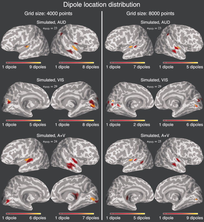
Left side: The dipole locations at the end of the chains for different stimulus types of SIMULATED data using the 4,000 grid size. The number of linearly independent measurement combinations for the SVD speed‐up strategy is also shown for different cases. Yellow color depicts areas where many of the chains had a dipole at the end and reddish color areas with fewer occurrences. Note that the scales vary and that this does not represent the posterior distribution of the samples, but only how the locations of different chains are distributed. Right side: Same as left side but for 8,000 grid size.

Figure 7.

Left side: The dipole locations at the end of the chains for different stimulus types of EMPIRICAL data using the 4,000 grid size. The number of linearly independent measurement combinations for the SVD speed‐up strategy is also shown for different cases. Yellow color depicts areas where many of the chains had a dipole at the end and reddish color areas with fewer occurrences. Note that the scales vary and that this does not represent the posterior distribution of the samples, but only how the locations of different chains are distributed. Right side: Same as left side but for 8,000 grid size.

The above equations need to be calculated once before the sampler is started, and as the L dimension of the parameters A _N, B, and C ${}_{\text{0}}^{\text{−1}}$ is reduced to n < L, the calculation time is substantially reduced. Note, that L should be replaced with n in the formulae, also.

Noise Covariance Estimate and Utilized Data

For the estimation of spatiotemporal noise covariance matrix C ₀, we used the multipair approximation [Jun et al.,2005; Plis et al.,2005]. For both empirical and realistically simulated data, we had ∼150 trial averages for the different stimulus types and over 1,500 noise trials recorded randomly from the off‐stimulus interval. The same, real noise fragments were used in both cases to have realistic noise covariance structure also for the simulated data (Fig. 1). The time‐consuming inverse of C ₀ was estimated using the methods described in Jun et al. [2005].

Figure 1.

The full spatiotemporal noise covariance structure is identical for both simulated and empirical data and it was estimated from the real raw data for both cases.

The MEG raw data were acquired with a sampling rate of 600 Hz and downsampled to 150 Hz, notch filtered for 50 Hz noise, and high‐pass filtered for slow drifting noise prior to the analyses. The empirical data consist of averaged evoked fields of auditory (AUD), visual (VIS), and simultaneous auditory and visual (A + V) stimuli presented every 4 s having ∼150 trials in each category not including the ones contaminated with electro‐oculogram artifacts. The frequency and length of the tones were 800 Hz and 80 ms, respectively, with 5 ms linear slope at both ends. The subject fixated on the visual stimuli which were small, square‐shaped, black‐white, center‐field checkerboards of equal duration. Time window used in the analysis with respect to the stimuli was 0…20 ms and the actual averaged evoked fields can be seen in Figure 1.

The timecourses for the simulated realistic sources, which were used to forward calculate the simulated data (with grid size: 16,000), were produced by averaging timecourses of few real data measurement sensors roughly above the corresponding cortical location. Fitting these timecourses, we set two deep almost dipolar sources on the anterior parts of Heschl's gyrus, one on each hemisphere, and two slightly extended patches on V1 of both hemispheres. The simulated source timecourses were scaled so that the maximum amplitude was 80 nAm for the auditory and 120 nAm for the visual locations regardless of the source extent (Fig. 2). Part of the off‐stimulus interval noise trials were added to the forward calculated fields to produce realistic spatiotemporal measurement noise for the simulations. The resulting simulated and empirical measurement averages have essentially same characteristics by visual inspection and the noise covariance structure is identical for both cases (Fig. 1).

Figure 2.

Top: Simulated source locations include small patches on the primary auditory and visual areas. The auditory patches contained two and visual patches ten source space points on the densest 16,000 grid. Dark shades of gray denote the sulci and light shades of gray the gyri. Bottom: The simulated source timecourses for each stimulus category were acquired by averaging few sensors of MEG evoked fields and scaled to a suitable value regardless of the source extent.

We also made a large set of data simulations with 1, 2, or 3 randomly positioned dipoles having 50 different configurations for each number of dipoles. Grid size of 4,000 was used for producing the data and grid sizes of 3,000 and 4,000 were used for inverse estimation. These simulations were done to evaluate the performance of the model with simple sources and determine how well the model can estimate the number of sources, as well as to further demonstrate the multimodality of the posterior distribution.

RESULTS

For the multiple simulated dipolar source configurations, one chain per source configuration was run and the resulting histograms of average number of dipoles for different solution configurations are shown in Figure 3. Most often, the model can determine the correct number of underlying dipoles although with larger number of dipoles (2–3) in several cases the obtained solution estimate has more than three dipoles. With one dipole (using the same grid for inverse), there seems to be an inconsistency as there might be two dipoles in the solution in about half the cases. However, if one looks at the dipole locations and samples, it is clear that the other dipole is in practice always in the correct location and the other is a spurious dipole that might appear and disappear as the sampling procedure advances (Fig. 5A).

Figure 3.

On the left side the grid used for inverse analysis was the same as the one used for forward calculating the measurements (4,000) and on the right side the grid size used for inverse analysis was coarser (3,000).

Figure 5.

The posterior samples of {θ,ϕ}‐coordinates of five different one dipole source configuration runs (A) and for all the runs of the auditory empirical dataset analyzed with grid size 4,000 (B). In each subfigure, the same color pair trendlines represent the ith {θ,ϕ}‐coordinate pair (i.e., one dipole).

Table I shows the mean goodness‐of‐fit values for the multiple source configuration results of the reduced measurement combinations using the SVD strategy as well as the goodness‐of‐fit when taking into account all the measurements. The localization error in 3‐D is calculated so that the errors of the closest estimated dipoles to the correct locations are summed together. The spurious dipoles that might emerge are not taken into account for this metric. When using the same grid for the inverse analysis (IC) the localization error is smaller than when using a different grid discretization. The goodness‐of‐fit values are good when computed using the full data even though the inverse analysis was performed only with the small set of linearly independent measurement combinations.

Table I.

The mean goodness‐of‐fit values of the multiple source configuration results for the full data and the linearly independent measurement combinations from the SVD‐strategy and the mean sum of localization errors for all the simulated dipoles in centimeters

	1 dip	2 dips	3 dips	1 dip (IC)	2 dips (IC)	3 dips (IC)
gof (full data)	0.85	0.95	0.96	0.86	0.96	0.96
gof (SVD)	0.93	0.97	0.97	0.91	0.98	0.97
loc error (cm)	0.67	0.82	1.94	0.16	0.36	1.54

For the audiovisual stimulus categories (AUD, VIS, A + V) of simulated and empirical data, we ran 10 chains with two of the coarser grid sizes (4,000 and 8,000). The starting point was selected randomly and 15,000 samples from each chain were drawn. The posterior energies of the chains are depicted in Figure 4. The time to draw 10,000 samples for one chain was about 1 h if the number of independent measurement combinations n _SVD = 20…30. The simulations were done during several days on few workstations, but using parallel computing methods, large number of chains for one category can be run in a reasonable amount of time making the method feasible also for studies with many subjects. For the analysis and sampling the timecourses for the solution modes, we utilized only 100 samples, uniformly thinned from the last 1,000 samples of each chain. Samples for the {θ,ϕ} parameters for all the runs of the empirical auditory dataset (grid size: 4,000) are shown in Figure 5B.

Figure 4.

Illustration of the energy of the posterior distribution at each step of our sampler. The chains converge rather rapidly to a local mode, but they get stuck easily and may jump to a mode having lower energy only after several thousands of samples.

By visual inspection of the obtained samples and posterior energies, it can be seen that the chains converge to a local mode rather quickly (i.e., few hundred samples) but it is very difficult to determine whether the chains have converged globally as they still might jump to a different mode after several thousands of samples. This is especially true with more complex cases having multiple underlying sources, such as the empirical cases. Figure 5B shows how the 10 separate chains do not jump or mix well between different modes, yet almost all of the runs seem to sample in a different mode than the others. There seems to be few consistent dipoles across all the modes, but there also exists spurious varying dipoles, which demonstrates the multimodality of the posterior. Even with the most simplest case when only one dipole was simulated the posterior is multimodal, which can be seen in Figure 5A. However, with the simple case of one or two dipoles, the correct location is consistently seen from the samples even though some spurious dipoles might emerge during sampling. Because of the unfortunate fact that the chains do not mix well between different modes, especially in the more complex cases, one cannot compare how much probability mass each mode has. In the following, we chose to consider the modes determined by the lowest posterior energy (highest probability) and consistent dipole locations across different runs being the best representative modes.

Figures 6 and 7 depict the dipole location distributions at the end of the different MCMC runs. For example, in the top part of Figure 6 (simulated, 4,000/8,000, AUD), it can be seen that with most chains the dipoles localize rather well on the correct simulated locations. Despite this, the posterior is clearly multimodal because different chains arrive at different locations. Evidently, the grid discretization size does not have a notable effect on the shape and behavior of the posterior, implicating that our model is not too sensitive to the accuracy of cortical constraints regarding different discretizations. Similar tendencies are seen with VIS and A + V categories as well. With empirical data (Fig. 7), the dipole location distributions are a bit more distributed meaning that the posterior tends to be even more multimodal. Also contributing to this, the visual stimuli were such that one would expect a large activation in the primary visual areas, which is difficult to model by few equivalent current dipoles and therefore may produce an extremely complex posterior having wide spectrum of local modes.

In most cases with simulated data, our method tends to explain the AUD and VIS categories with two dipoles (Fig. 8). Most chains of simulated A + V ended in a mode having only three dipoles, although there were four dipoles in the actual simulation. This, together with the results with multiple simulated dipolar source configurations (Fig. 3), shows that with higher number of sources, the shape of the posterior distribution landscape gets more complicated and spiked, suggesting that our model has difficulties in coping well with larger number of sources. Also, with increasing number of underlying dipoles, the distribution of the locations gets more diffused (Fig. 6). With empirical data, the model tries to explain the AUD and VIS categories with higher number of dipoles than in the simulated case, suggesting that the simple auditory and visually elicited responses cannot be adequately explained with only two spatially static and temporally varying dipoles. In the visual case, the true activation may be more widespread and therefore the model might try to explain those sources with only a few dipoles that compensate for the complex activation patterns on the opposite walls of the visual cortices. With some of the modes this is the case (Fig. 11). Similarly to the situation with simulated data, the posterior gets more multimodal when there are more underlying sources generating the data. Thus, the possible inferences made from the posterior with the current model become much more ambiguous with complex sources.

Figure 8.

The distribution of the number of dipoles at the end of the chains for simulated and empirical audiovisual data.

Figure 11.

Representative best solution mode (lowest posterior energy) for empirical visual source using 8,000 grids. In this solution mode, there are two solution dipoles, one of which is on the left V1 (red dipole), and the other is located on the right V1 (blue dipole). We obtained several other modes with the visual category yielding results having two or three dipoles located either as in this mode or bit more superficially, so that on one hemisphere there are two dipoles, which do not land directly on V1 or V2. In such case, the two dipoles probably just compensate for the large‐scale and widespread activation pattern of primary visual areas. This suggests that as several different modes produce similar and good data fits, the underlying source is far more complicated than two or three dipolar sources.

Figures 9, 10, 11 show a best representative mode in some of the categories having the lowest posterior energy. The localization accuracy with the simulated data is good, and with empirical data, the obtained dipole locations seem plausible. The results with the best modes from other cases and modes having slightly higher posterior energies are not visualized here, but they yielded similar results although showing the multimodality of the posterior distribution.

Figure 9.

Representative best solution mode (lowest posterior energy) for simulated auditory source using 8,000 grid. The original source on the left hemisphere (magenta patch) is mislocalized (red dipole) to a neighboring deeper gyrus and, therefore, the orientation is opposite and the solution amplitude larger as more current is needed to produce the same fields from a deeper location. The standard deviation of the current samples (dashed lines) do not reveal the great difficulty in the multimodality of the posterior as it only gives information of this particular mode. The data fit to all 198 measured gradiometer channels and 31 timepoints produced by the solution is good given that only n _SVD = 23 measurement combinations were used in the inverse analysis.

Figure 10.

Representative best solution mode (lowest posterior energy) for empirical auditory source using 8,000 grids. This solution mode suggests that there is an earlier more superficial source (green dipole) and a later deeper source (red dipole) on the left hemisphere and one earlier source (blue dipole) on the right hemisphere. The data fit is adequate although there are some differences between the measured and forward calculated fields.

We tried the model without the SVD speed‐up and regularization strategy with some simulations as well, but in that case the sampling was extremely slow and would not suit practical purposes even though the resulting modes were similar to the ones presented here in the results. Notably, the data fits that were forward calculated for all the measured fields are rather good in all cases even though the solution estimates were calculated only using 20…60 independent measurement combinations.

DISCUSSION

We implemented a Bayesian method for localizing MEG data with cortically constrained multiple dipoles. The model was based on a previous one proposed by Jun et al. [2005], but as new features we utilized individual anatomical cortical location and orientation constraints. Also, we performed the MCMC sampling on the spherically inflated cortical surfaces represented with two angle coordinates. This transformation is of use with methods that require the parameter space sampled to be continuous and bounded. Furthermore, we utilized the truncated singular value decomposition to include only some of the largest linearly independent measurement combinations to speed up and regularize the sampling scheme. We tested the method with both empirical and simulated MEG data sets.

Unfortunately, at least with strict orientation constraints, our sampler does not mix well between local modes and therefore the mapping of the full posterior distribution becomes extremely difficult as it is clearly highly multimodal. This creates a problem as comparing the posterior energies of different chains does not reveal anything of the probability mass of the corresponding mode. Therefore, one must be very careful when comparing only the posterior energies and consistent source locations across modes. Although with limitless computational resources, the multimodality could be attacked by, for example, importance sampling and resampling strategies to reveal the mass proportions of the different modes; to our experience, it may not be worth the effort to try to improve the sampler at this point. Instead, the current model might be elaborated by utilizing loose [Lin et al.,2006] or fully free orientation constraints. As the original model by Jun et al. [2005], which utilized a spherical head model and volumetric source space, showed good results without the use of orientation constraints, loosening the rigid constraint might improve the mixing properties of the sampler and the model would still have the advantages of cortical location and loose orientation constraints.

Other than being automatic, these kinds of methods have many other advantages in comparison to traditional handmade trial‐and‐error type of use of equivalent current dipoles. The incorporation of fMRI priors or any other suitable prior information for that matter is very easy to implement and we are currently pursuing our efforts to that direction. Also, if the full posterior distribution could be extensively charted, the inference would give better measures of the validity of the many possible solutions and their probabilities rather than just simple goodness‐of‐fit values or posterior energies.

On the other hand, it seems that even the simple auditory or visually elicited responses are produced by rather complex sources and are not easily modeled with few dipoles or at least in many cases an experienced researcher does the job better than a robust automatic method. Still, in developing these, an interesting idea would be to include a prior to the model explaining the background brain noise, which would let the method itself model both the most prominent dipolar sources and more widespread background activity. Another possible way to improve the model would be to increase the sampled parameters by one describing the extent of the dipole and have a joint dipole and extended region model. This might improve the modeling of sources to larger extent, such as the ones elicited by large or even full‐field visual stimuli.

The question of how much we lose information in the data by using the SVD speed‐up and regularization strategy remains partially open. We did try the method without the SVD strategy and it produced similar results. However, more systematic examination of this would have required a vast amount of computational time and it was not feasible in the scope of this study. Given that the approximate distance between the MEG measurement sensors is about 35 mm and the minimum distance of a sensor from the scalp is almost 20 mm, it is reasonable to assume that the gradiometers measure at least partially the same phenomena and, thus, dropping of the smallest linearly independent measurement combinations is justifiable and by doing this we are not at least fitting the solution to measurement noise. Note, that for computational reasons the current model uses only the ∼200 gradiometer measurements but with the cost of computational speed we should be readily able to include ∼100 magnetometer measurements to provide more information of the underlying sources. Naturally, there are some practicalities to be solved in performing the speed‐up strategy jointly to two different types of measurement sensors.

In a recently proposed hierarchical Bayesian generalization of the traditional MNE, the variance parameter of each cortical source space point is considered as a random variable and estimated from the data. This estimation task can be done using the variational Bayesian framework or by Monte Carlo sampling. For a detailed description and simulation results on the VB‐method, the reader is instructed to revise the previous works by Sato et al. [2004] and Nummenmaa et al. [2006]. The hierarchical MNE produces rather robust estimates of the MEG inverse problem that could serve as a starting point and a mask to restrict the source space to specific locations on the cortex. Our present multiple dipole sampler could then be used to place dipoles on these confined areas. This way, we may be able to overcome the poor switching of the modes of the sampler and, by using loose orientation constraints, adequately and relatively fast map the posterior in the prelocalized areas. The implementation and testing of this hybrid model is left to ongoing research.

CONCLUSION

We showed that the presented implementation for localizing multiple dipoles with cortical orientation and location constraints produces good inverse estimates albeit suffering from the multimodality of the posterior and poor mixing of the sampler making it difficult to theoretically compare the different inverse estimate modes. As a new approach, we introduced the sampling to be done on spherical angle coordinates of the hemispheric locations continuously in two dimensions. As future improvements to our model we suggest using fMRI priors, loose orientation constraints and, as dipoles are not always the best representatives of the underlying sources, usage of extended regions so that a dipolar source would be a special case of a shrunken region. Finally, we briefly sketch out a possibility to construct a hybrid model composed of prelocalization and masking step done with a variational Bayesian hierarchical minimum‐norm estimate, and a sampling step in which some efficient dipole/extended region sampler is used to explore the posterior distribution in the local area.

APPENDIX A: MARGINALIZATION OF C AND J_N

To marginalize away the noise covariance parameter C and source current parameter J _N, we follow the steps of Jun et al. [2005]. We do not show all the phases of the calculations as it would be pointless replication of previously published work. Instead, we verbally describe the procedure and show some intermediate results to convince the interested reader of the calculations and to set grounds for showing how the SVD speed‐up and regularization strategy is incorporated in the model (see, Appendix B). Note, that possibly due to a typographical error in the original derivation of the marginalization of J _N in Jun et al. [2005], the term was missing in some parts of their calculations.

The marginalization of C is done by rearranging Eq. (11) into (k + 1)th inverted Wishart distribution having in the place of C ₀. The integral over the probability distribution is simply the reciprocal of the normalization constant of this Wishart distribution. Substituting back Ĉ ₀, and taking into account the symmetry and positive definiteness of C ₀ in the manipulations, we arrive at

(21)

The marginalization over J _N is also done using normalization property of probability distribution function. Consider only the part of Eq. (21) containing parameter J _N:

(22)

By defining and opening B _n, we get

Further on, the expression in the brackets [·] is equivalent to

(23)

The latter parts containing J _N can be rearranged (completing to a square) by using matrix inversion lemma and noting that vec(J _N A _N) = (A _N ^T ⊗ I _T)vec(J _N), leading finally to

where q, C ₁, and r are like in the attributes of Eq. (12). Equation (22) can now be written to a form, where an approximation of (1 + ψ)^−p ≈ e ^−pψ can be used and the result can be arranged to a normal distribution for vec(J _N). By including the front part of Eq. (21), we get the posterior distribution from which J _N is marginalized out:

(24)

Dropping the constants from this yields the final posterior distribution of the parameters shown in Eq. (12). Realizations of vec(J _N) can be drawn from Eq. (13).

APPENDIX B: EFFECT OF SVD ON A_N, B, AND C${}_{\text{0}}^{\text{−1}}$

Equation (23) in Appendix A contains the only occurrences of A _N and B in the expression for the posterior distribution. By substituting Eqs. (16) and (17) to this, we obtain

(25)

By using [Harville (1999), Chapter 16.2]

we can further process Eq. (25) to the form

(26)

Now, it is straightforward to define the inverse of the reduced noise covariance matrix as

and arrive at Eq. (23) with A _N, B, and C ${}_{\text{0}}^{\text{−1}}$ defined as in Eqs. (18), (19), (20). The rest of the model derivation goes as elsewhere.

REFERENCES

- Auranen T,Nummenmaa A,Hämäläinen MS,Jääskeläinen IP,Lampinen J,Vehtari A,Sams M ( 2005): Bayesian analysis of the neuromagnetic inverse problem with ℓp‐norm priors. Neuroimage 26: 870–884. [DOI] [PubMed] [Google Scholar]
- Baillet S,Garnero L ( 1997): A Bayesian approach to introducing anatomo‐functional priors in the EEG/MEG inverse problem. IEEE Trans Biomed Eng 44: 374–385. [DOI] [PubMed] [Google Scholar]
- Baillet S,Mosher JC,Leahy RM ( 2001): Electromagnetic brain mapping. IEEE Signal Process Mag 18: 14–30. [Google Scholar]
- Bernardo JM,Smith AFM ( 1994): Bayesian Theory. Chichester: Wiley. [Google Scholar]
- Bertrand C,Ohmi M,Suzuki R,Kado H ( 2001): A probabilistic solution to the MEG inverse problem via MCMC methods: The reversible jump and parallel tempering algorithms. IEEE Trans Biomed Eng 48: 533–542. [DOI] [PubMed] [Google Scholar]
- Dale AM,Sereno MI ( 1993): Improved localization of cortical activity by combining EEG and MEG with MRI cortical surface reconstruction: A linear approach. J Cogn Neurosci 5: 162–176. [DOI] [PubMed] [Google Scholar]
- Dale AM,Fischl B,Sereno MI ( 1999): Cortical surface‐based analysis. I. Segmentation and surface reconstruction. Neuroimage 9: 179–194. [DOI] [PubMed] [Google Scholar]
- Dale AM,Liu AK,Fischl BR,Buckner RL,Belliveau JW,Lewine JD,Halgren E ( 2000): Dynamic statistical parametric mapping: Combining fMRI and MEG for high resolution imaging of cortical activity. Neuron 26: 55–67. [DOI] [PubMed] [Google Scholar]
- Fischl B,Sereno MI,Dale AM ( 1999): Cortical surface‐based analysis. II. Inflation, flattening, and a surface‐based coordinate system. Neuroimage 9: 195–207. [DOI] [PubMed] [Google Scholar]
- Friston KJ,Glaser DE,Henson RNA,Kiebel S,Phillips C,Ashburner J ( 2002a): Classical and Bayesian inference in neuroimaging: Applications. Neuroimage 16: 484–512. [DOI] [PubMed] [Google Scholar]
- Friston KJ,Penny W,Phillips C,Kiebel S,Hinton G,Ashburner J ( 2002b): Classical and Bayesian inference in neuroimaging: Theory. Neuroimage 16: 465–483. [DOI] [PubMed] [Google Scholar]
- Gelman A,Carlin JB,Stern HS,Rubin DB ( 2003): Bayesian Data Analysis, 2nd ed. London: Chapman & Hall. [Google Scholar]
- Gilks WR,Richardson S,Spiegelhalter DJ ( 1996): Markov Chain Monte Carlo in Practice. London: Chapman & Hall. [Google Scholar]
- Green PJ ( 1995): Reversible jump Markov chain Monte Carlo computation and Bayesian model determination. Biometrika 82: 711–732. [Google Scholar]
- Gupta AK,Nagar DK ( 2000): Matrix Variate Distributions. Monographs and Surveys in Pure and Applied Mathematics. London: Chapman & Hall; pp. 111–113. [Google Scholar]
- Hämäläinen MS,Ilmoniemi RJ ( 1984): Interpreting measured magnetic fields of the brain: Estimates of current distributions. Technical Report TKK‐F‐A559,Department of Technical Physics, Helsinki University of Technology, Espoo, Finland.
- Hämäläinen MS,Sarvas J ( 1989): Realistic conductivity geometry model of the human head for interpretation of neuromagnetic data. IEEE Trans Biomed Eng 36: 165–171. [DOI] [PubMed] [Google Scholar]
- Hämäläinen MS,Hari R,Ilmoniemi RJ,Knuutila J,Lounasmaa OV ( 1993): Magnetoencephalography—Theory, instrumentation, and applications to noninvasive studies of the working human brain. Rev Mod Phy 65: 413–497. [Google Scholar]
- Hansen PC ( 1987): The truncated SVD as a method for regularization. BIT Numerical Math 27: 534–553. [Google Scholar]
- Harville DA ( 1999): Matrix Algebra from a Statistician's Perspective. Berlin: Springer‐Verlag. [Google Scholar]
- Hauk O ( 2004): Keep it simple: A case for using classical minimum norm estimation in the analysis of EEG and MEG data. Neuroimage 21: 1612–1621. [DOI] [PubMed] [Google Scholar]
- Jun SC,George JS,Paré‐Blagoev J,Plis SM,Ranken DM,Schmidt DM,Wood CC ( 2005): Spatiotemporal Bayesian inference dipole analysis for MEG neuroimaging data. Neuroimage 28: 84–98. [DOI] [PubMed] [Google Scholar]
- Kaipio JP,Somersalo E ( 2005): Statistical and Computational Inverse Problems. New York: Springer. [Google Scholar]
- Kincses WE,Braun C,Kaiser S,Grodd W,Ackermann H,Mathiak K ( 2003): Reconstruction of extended cortical sources for EEG and MEG based on a Monte‐Carlo‐Markov chain estimator. Hum Brain Mapp 18: 100–110. [DOI] [PMC free article] [PubMed] [Google Scholar]
- Köhler T,Wagner M,Fuchs M,Wischmann HA,Drenckhahn R,Theissen A ( 1996): Depth normalization in MEG/EEG current density imaging. In Proceedings of the 18th Annual International Conference of the Engineering in Medicine and Biology Society of the IEEE, Amsterdam, October 31–November 3, 1996.
- Lin FH,Belliveau JW,Dale AM,Hämäläinen MS ( 2006): Distributed current estimates using cortical orientation constraints. Hum Brain Mapp 27: 1–13. [DOI] [PMC free article] [PubMed] [Google Scholar]
- Liu AK,Belliveau JW,Dale AM ( 1998): Spatiotemporal imaging of human brain activity using functional MRI constrained magnetoencephalography data: Monte Carlo simulations. Proc Natl Acad Sci USA 95: 8945–8950. [DOI] [PMC free article] [PubMed] [Google Scholar]
- Matsuura K,Okabe Y ( 1995): Selective minimum‐norm solution of the biomagnetic inverse problem. IEEE Trans Biomed Eng 42: 608–615. [DOI] [PubMed] [Google Scholar]
- Mosher JC,Leahy RM,Lewis PS ( 1999): EEG and MEG: Forward solutions for inverse methods. IEEE Trans Biomed Eng 46: 245–259. [DOI] [PubMed] [Google Scholar]
- Mosher JC,Lewis PS,Leahy RM ( 1992): Multiple dipole modeling and localization from spatio‐temporal MEG data. IEEE Trans Biomed Eng 39: 541–557. [DOI] [PubMed] [Google Scholar]
- Neal RM ( 2003): Slice sampling. Ann Stat 31: 705–767. [Google Scholar]
- Nummenmaa A,Auranen T,Hämäläinen MS,Jääskeläinen IP,Lampinen J,Sams M,Vehtari A: Hierarchical Bayesian estimates of distributed MEG sources: Theoretical aspects and comparison of variational and MCMC methods, NeuroImage (2007), doi: 10.1016/j.neuroimage.2006.05.001 (in press). [DOI] [PubMed] [Google Scholar]
- Okada YC,Wu J,Kyuhou S ( 1997): Genesis of MEG signals in a mammalian CNS structure. Electroencephalogr Clin Neurophysiol 103: 474–485. [DOI] [PubMed] [Google Scholar]
- Phillips JW,Leahy RM,Mosher JC ( 1997): MEG‐based imaging of focal neuronal current sources. IEEE Trans Med Imaging 16: 338–348. [DOI] [PubMed] [Google Scholar]
- Plis SM,George JS,Jun SC,Paré‐Blagoev J,Ranken DM,Schmidt DM,Wood CC ( 2005): Spatiotemporal noise covariance model for MEG/EEG data source analysis. Technical Report LAUR‐043643,Los Alamos National Laboratory, Los Alamos, New Mexico.
- Råde L,Westergren B ( 1998): Mathematics Handbook for Science and Engineering. Lund: Studentlitteratur. [Google Scholar]
- Robert CP,Casella G ( 2004): Monte Carlo Statistical Methods, 2nd ed. New York: Springer. [Google Scholar]
- Sarvas J ( 1987): Basic mathematical and electromagnetic concepts of the biomagnetic inverse problem. Phys Med Biol 32: 11–22. [DOI] [PubMed] [Google Scholar]
- Sato MA,Yoshioka T,Kajihara S,Toyama K,Goda N,Doya K,Kawato M ( 2004): Hierarchical Bayesian estimation for MEG inverse problem. Neuroimage 23: 806–826. [DOI] [PubMed] [Google Scholar]
- Schmidt DM,George JS,Wood CC ( 1999): Bayesian inference applied to the electromagnetic inverse problem. Hum Brain Mapp 7: 195–212. [DOI] [PMC free article] [PubMed] [Google Scholar]
- Schmidt DM,George JS,Ranken DM,Wood CC ( 2000): Spatial‐temporal Bayesian inference for MEG/EEG. In Proceedings of the 12th International Conference on Biomagnetism, Espoo, Finland. http://biomag2000.hut.fi/papers/0671.pdf.
- Uutela K,Hämäläinen MS,Somersalo E ( 1999): Visualization of magnetoencephalographic data using minimum current estimates. Neuroimage 10: 173–180. [DOI] [PubMed] [Google Scholar]