Functional imaging analysis contest (FIAC) analysis according to AFNI and SUMA

Abstract

The Functional Imaging Analysis Contest (FIAC) datasets were analyzed with the AFNI software package. Two types of linear regression analyses were carried out: “fixed shape” hemodynamic response, where a preselected incomplete gamma function is used to model each brief activation episode, and “variable shape” analysis, where the temporal shape of the response model in each stimulus block class is allowed to vary separately in each voxel. These time series regressions were carried out both in the volume and on the original data projected to individual standardized cortical surface models. Intersubject analyses were carried out voxel‐wise on the regression amplitudes obtained from these time series results, using a multi‐way within‐subject analysis of variance (ANOVA). Group analysis of the block design demonstrated a significant repetition suppression of the BOLD signal within blocks in the superior and middle temporal gyrus. This effect may represent differences in the response to the first stimulus following a period of silence compared to the remaining sentences in the block. Analyzing the event‐related data, Brodmann area 31 showed significant sentence effect and consecutive‐sentence repetition effect. However, no significant speaker effect was found; these results may be consistent with the instructions to the subjects that they would be tested on the sentence content. Sentence by speaker interaction effects were found in bilateral middle temporal gyrus, left inferior frontal, and left inferior temporal gyrus. Hum Brain Mapp, 2006. © 2006 Wiley‐Liss, Inc.

INTRODUCTION

The Functional Imaging Analysis Contest (FIAC) data [Dehaene‐Lambertz et al., 2006] was analyzed in several ways using AFNI and SUMA. Block and event‐related design data were modeled using two kinds of linear regression models: “fixed shape” hemodynamic response, where a preselected incomplete gamma function is used to model each brief activation episode, and “variable shape” analysis, where the temporal shape of the response model in each stimulus block class is allowed to vary separately in each voxel. For each voxel the fixed shape analysis results in a single response amplitude for each stimulus class. For the block design only, the variable shape analysis modeled the response in each stimulus class as a piecewise linear function. In the block design, regression coefficients that formed the response function were used in a 3‐way within‐subject analysis of variance (ANOVA) with factors of sentence, speaker, and time‐after‐block‐onset as fixed effects, and subject as a random effect. We tested for main effects of each of the fixed factors and their interactions. Using variable shape regression results, we also tested for the significance of a contrast modeling a linear trend during each block type. We performed conjunction analysis for both main effects and trends of the four stimulus categories. For the event‐related data, we used a similar 2‐way within‐subject ANOVA to test for main effects of sentence and speaker and their interactions.

The open‐source AFNI software package [Cox, 1996; Cox and Hyde, 1997] has grown over the years into a suite for analysis and visualization of functional MRI (fMRI) data. The interactive AFNI program provides the ability to display datasets defined over 3‐D and 4‐D grids, showing slices, time series graphs, and volume rendering. The interactive SUMA program provides the ability to display datasets defined over triangulated 2‐D manifolds embedded in 3‐D space (i.e., cortical surface models). All these display modes are linked together interactively; for example, clicking on an activation “blob” on a surface display in SUMA will cause a corresponding time series display to jump to the corresponding location in AFNI. (The figures presented herein are screenshots from AFNI and SUMA.) This feature allows a researcher to “surf” through data, viewing results both quickly and comprehensively. The core analysis programs in the AFNI collection can carry out node‐wise statistical analyses on datasets defined over 2‐D surface or 3‐D volumetric spatial domains; software tools exist to project data from 3‐D volumes to 2‐D surfaces and back.

The analysis sequences are briefly outlined below, and relevant images are shown to illustrate the results. Program names are mentioned where appropriate to facilitate the finding of more detailed information from the website (http://afni.nimh.nih.gov). Some discussion of the experiment and results is presented at the end.

MATERIALS AND METHODS

MRI Data and Auditory Stimulation

We will not recapitulate all the data acquisition and stimulus details [Dehaene‐Lambertz et al., 2006], but a few salient points need mentioning. In this article we define an “imaging run” as the time series of 195 volumes obtained simultaneously during one 8.125‐minute stimulus presentation period. We processed data from 12 of the 15 subjects. The three subjects dropped from the analysis due to various problems during data acquisition were numbers 5, 10, and 12 (incomplete scans, sleeping, and coughing, respectively).

Subjects were instructed to listen attentively to sentences while lying still, eyes closed in the scanner. They were told to expect a recall test, after the scan, on some of the sentences they heard (it is unclear if there was an incentive for good performance; until very recently, there were no test result data on the FIAC web site, so the analyses below do not include any allowance for subject‐specific test performance). In all, 640 sentences were presented by 10 readers (5 men, 5 women) with sentences lasting on average 2277 ms. In the block design experiment, six sentences were presented, one every 3333 ms, for a block duration of 20 seconds, followed by a 9‐second interval of silence. There were 4 types of blocks:

• SSt‐SSp: Same consecutive Sentences, Same Speaker

• SSt‐DSp: Same consecutive Sentences, Different Speaker

• DSt‐SSp: Different consecutive Sentences, Same Speaker

• DSt‐DSp: Different consecutive Sentences, Different Speaker

Each subject was scanned for 2 block runs comprising 16 blocks each (4 of each class). The same types of sentence/speaker sequences were also adapted to an event‐related design (also 2 runs per subject).

Volume‐Based Preprocessing

Anatomical and EPI datasets were converted from ANALYZE 7.5 to AFNI's native 3‐D and 4‐D format (program 3dcopy). EPI time series data were corrected for slice timing offset (program 3dTshift). Six‐parameter rigid body inter‐ and intrarun motion correction was performed whereby volumes in the EPI scans were registered to the EPI volume that was acquired most closely in time to the high‐resolution MPRAGE anatomical scan (program 3dvolreg). This step was followed by automated transformation of the 3‐D anatomical and 4‐D time series datasets to Talairach‐Tournoux standard space using modified templates for T1 (from MNI: http://www.bic.mni.mcgill.ca/) and EPI (from SPM: http://www.fil.ion.ucl.ac.uk/spm) (program 3dWarpDrive). The templates were modified to correspond with the Talairach coordinate system [Talairach and Tournoux, 1988] instead of the MNI space. EPI time‐series were scaled by the mean at each voxel and volumes were then smoothed with 4‐mm and 8‐mm full‐width at half‐maximum (FWHM) Gaussian kernels for block and event‐related design data, respectively (program 3dmerge).

Surface‐Based Preprocessing

Surface models from each subject's T1 volume were created using FreeSurfer [Dale et al., 1999] and warped to a spherical template [Fischl et al., 1999a]. Standardization of surface meshes was then performed to create a node‐to‐node correspondence across surfaces from multiple subjects [Saad et al., 2004] (program MapIcosahedron). After mapping the time series data to the standard‐mesh cortical surfaces and applying surface‐based smoothing (programs 3dVol2Surf, SurfSmooth), the analyses proceeded much in the same way as for voxel‐based analysis, except for the clustering operations.

Linear Regression

Block and event‐related design data were modeled using two kinds of linear regression models (program 3dDeconvolve). The “fixed shape” models for both the block and event‐related designs were generated by convolving the timing of each stimulus class with an incomplete gamma function that approximates the BOLD response to events that are on the order of a second or more. For each voxel, the fixed shape analysis results in a single response amplitude for each stimulus class. For the block design only, the “variable shape” analysis modeled the response in each stimulus class as a piecewise linear function (the sum of “tent” or piecewise linear B‐spline basis functions with a collective support lasting 28 s after the start of the block). Figure 1 illustrates the modeling of the BOLD response to an event using a weighted sum of spaced‐apart linear B‐spline functions. Typically, each tent spans an interval of 2 TR periods, and the number of tents depends on the expected duration of the response to the event. In Figure 1, 5 tent functions are illustrated, but for the study we used 12 to cover the entire duration of a block plus enough time for the BOLD signal to return to baseline level. Thus, for each voxel the variable shape analysis results in 12 amplitudes for each stimulus class; these results are used to estimate and graph the actual time course of the response to each stimulus class, which can then be tested for shape differences (e.g., late EPI signal different from early EPI signal? or, does the response trend downwards during a block? cf. Fig. 3) as well as testing for overall block amplitude differences between classes. Note that the response estimated using the tent functions reflects the convolution of the hemodynamic impulse response function and the neuronal response function to a particular event. To make inferences about one of the contributing response functions requires either fixing or separately estimating the other.

Figure 1.

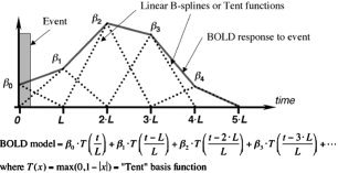
Illustration of the use of tent or linear B‐spline functions to model the BOLD response to an event.

Figure 3.

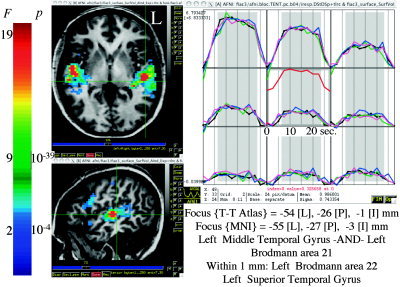
Sample regression results from Subject 3. Left column: Axial and sagittal slices through areas activated during the block design task. The colors encode for the omnibus F test for the regressors of interest. Equivalent voxel‐wise P values are shown to the right of the color scale. Corrected P value for activation maps was less than 0.05. An anatomical annotation text panel, modified here for readability, tracks the location of the crosshair in Talairach space. The letters R, L, I, S, A, and P are codes for the 6 cardinal directions. The tracking works whether navigation occurs on the surface or in the volume. The graphs matrix shows the reconstruction of the BOLD response, in a 3 × 3 voxel area centered on the crosshair. Black lines show the response during the DSt‐DSp block using the tent basis functions. The red overlay function, offset to the top of the central graph for clarity, shows the average response for the nine DSt‐DSp time series shown. The other colored graphs represent the estimated responses from the 3 other conditions. All images are in radiological view such that left is right and right is left.

In addition to the regressors that modeled the response to the stimulus, we used regressors to model motion residuals, and modeled baseline drifts using quadratic polynomials in time for each separate imaging run (12 time series regressors of no interest total for the 2 runs in each analysis). The correction for multiple comparisons was made by rejecting spatial clusters smaller than what would be expected by chance using Monte‐Carlo simulations [Forman et al., 1995], given a voxel‐wise false‐positive level (program AlphaSim). Given the spatial smoothness of the data, the number of brain voxels, and the voxel‐wise probability of false‐positives, the program estimates the probability of obtaining clusters of a particular size by chance alone (false positive) using a simulation approach.

Group Analysis

In the block design, regression coefficients that formed the response function were used in a 3‐way within‐subject ANOVA with factors of sentence (same vs. different), speaker (same vs. different), and time‐after‐block‐onset (seven levels) as fixed effects, and subject as a random effect (program GroupAna). We tested for main effects of each of the fixed factors and their interactions. We also tested for the significance of a contrast modeling a linear trend of the nine time points of each response that are highlighted in gray in Figure 3 using the variable shape analysis regression results. Linear trend tests were conducted separately for each of the four conditions. Thresholding, whenever applicable, was performed by setting the statistical parameter to a value resulting, in conjunction with cluster size, in a corrected P < 0.05 (minimum cluster size of 8 voxels, 288‐μL, volume of 1 EPI voxel at original resolution is 36 μL). We performed conjunction analysis for both main effects and trends of the four stimulus categories (program 3dcalc).

For the event‐related data, we used a 2‐way within‐subject ANOVA to test for main effects of sentence and speaker and their interactions. Statistical thresholds were set in a manner similar to that for the block design.

RESULTS

Single‐Subject Results

Figure 2 shows single subject results for Subject 3. The top images show the left and right views of a surface model of the gray–white matter border for this subject. The middle images show the omnibus F statistic including all stimulus‐related regressors for the block design data overlaid on inflated models of the surfaces on the top. Because cortical folding obscures the display of functional activation in the depths of sulci, this subject's functional data are presented overlaid on an inflated model of the cortical surface. Inflated models offer several advantages for data presentation. The dark shading highlights the fundus of the sulci seen in the folded‐up surfaces. This method of rendering the data allows appreciation of the entire, unthresholded pattern of activation in the cerebral cortex while still retaining anatomical information in the form of sulcal highlights. Clusters of subthreshold activation would be readily visible, alerting the experimenter to results that might go undetected due to low statistical power. The bottom images show the omnibus F statistic from the event‐related data with a coloring scheme that is similar to the preceding panels. The event‐related data activated foci similar to those in the block design data; however, as expected, activation was considerably stronger in the block design runs. The common clusters of activation are in the superior temporal gyrus/sulcus (STG, STS) (Brodmann areas: BA 21, 22), the inferior frontal gyrus (IFG) (BA 44), and the medial frontal gyrus (MFG) (BA 11). Note that of these foci, only the temporal area survived in the final group analysis maps, highlighting the strong intersubject variability of the activation patterns.

Figure 2.

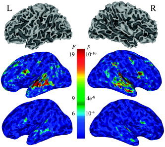
Top: Left and right surface models of the gray–white matter interface for Subject 3. Surface models were created using FreeSurfer (http://surfer.nmr.mgh.harvard.edu) and data processing and viewing using SUMA, AFNI's surface rendering program. Middle: Inflated versions of the models on the top. The colors reflect the omnibus F‐statistic from the block design data. Dark reds represent F‐statistics > 19 (P < 10⁻¹⁶, uncorrected), green F > 9 (P < 4 × 10⁻⁸, uncorrected), and light blues represent F‐statistics > 6.4 (P < 10⁻⁴, uncorrected). Data are from Subject 3. Bottom: Same as middle section, for event‐related design data. The statistical results shown in this figure were obtained by processing time‐series data mapped directly onto the cortical surface models. This rendering mode is complementary to the voxel‐based rendering modes in AFNI with an interactive linkage for navigation and data mapping.

For the results shown in Figure 2, the statistical analysis was performed in its entirety on the surface using the time‐series data projected from the volumes to the surface by integrating across the gray matter and then smoothed on the surface. The integration is done along directions formed by corresponding nodes from the gray–white border and pial surfaces (program Vol2Surf). This procedure was done to illustrate the possibility of performing node‐based rather than voxel‐based computations in AFNI and SUMA. Group analysis can also readily be done on the surfaces using the same software tools; however, we chose to bypass surface‐based group analysis because high‐quality anatomical datasets (an average of multiple T1‐weighted acquisitions) are needed to create accurate cortical surface models. With high‐quality anatomical data and good alignment between EPI and anatomy, surface‐based analysis can be advantageous relative to volume‐based methods. For expositions of the methods and considerations for carrying out surface‐based group analysis, see [Argall et al., 2006; Fischl et al., 1999b; Saad et al., 2004; Van Essen, 2002,2005].

The block design results shown in Figure 2 were obtained using four separate regressors that modeled each of the separate tasks—the fixed shape analysis described earlier. However, this simple model does not allow us to make inferences about intrablock stimulus repetition effects or other changes in response amplitude during a block. The variable shape analysis is designed for such purposes. Figure 3 shows sample results from Subject 3. The images on the left show axial and sagittal slices through the BA 21/22, with significant activation shown in the color overlay. The text panel shows the dynamic reporting (feature “whereami”) of the spatial location of the crosshair in Talairach space, using the Talairach Daemon database [Lancaster et al., 2000]. It is worth noting that this anatomical annotation window follows the crosshair location in real time, whether in the volumetric data or on surface models such as those in Figure 2. Other atlases, such as the cytoarchitectonic ones distributed by Zilles and colleagues [Amunts and Zilles, 2001; Zilles et al., 2002] are also available. Colors represent the range of F‐statistics for the full model (all stimulus‐related regressors). Thresholding was done using an F(56,314) value of 2.01 (blue colors) and a cluster size of 288 μL, resulting in a corrected P < 0.05. The array of graphs shows the estimate of the BOLD response (output of “variable shape” regression analysis) in a 3 × 3 voxel area centered on the crosshair. Black lines show the response during the DSt‐DSp block reconstructed using the tent basis functions. The red function in the central graph shows the average response for the nine DSt‐DSp time series shown. The other colored graphs represent the responses from the three other conditions. This makes for very efficient perusal of the various responses throughout the brain. Visual inspection of the responses in this area does not reveal any differences between the tasks. This is further considered by the trend analysis (below).

To investigate repetition effects, we examined the trends in the response amplitude in the period excluding the initial signal rise and final return to baseline. This period is highlighted in gray on the graphs, from 7.5 to 22.5 seconds following the first sentence of the block. Trend analysis was performed for a single subject (#3 shown here) and for the entire group. Although some of the graphs selected in Figure 3 do show a slight decreasing trend with repetition, no significant trends were found in the single‐subject case.

Group Analysis: Block Design

The group analysis was performed using the 3‐way ANOVA described above. The coefficients entered into the ANOVA were the estimates of the BOLD percent signal change during the interval shaded in gray in Figure 3 (7.5–22.5 seconds after block start). Figure 4 shows results of t tests performed to determine areas of the brain activated by stimulus class DSt‐DSp. The other 3 stimulus classes resulted in very similar activation areas located mostly in the STG/STS, BAs 21, 22, and 42. Conjunction analysis performed to examine the spatial overlap of the activation patterns revealed that 58% of the voxels overlapped in at least 3 of the 4 stimulus categories (76% overlapped in at least 2 of 4).

Figure 4.

Results of t tests performed to determine areas of the brain activated by stimulus class DSt‐DSp for both left and right hemispheres. The remaining three stimulus classes resulted in very similar patterns. Activation areas were mostly in bilateral STG/STS, BAs 21, 22, 42. The anatomical dataset of Subject 3 was used to display group results in this and following figures.

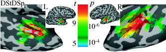
The montage images in Figure 5 shows all areas with significant intrablock repetition effects (slopes in the BOLD response during a block) for each of the 4 stimulus types. Only areas that showed significant activation (sentence effect or speaker effect, Fig. 4) are reported here. For all 4 conditions, significant negative repetition trends (P < 0.05, corrected) were observed bilaterally in superior and middle temporal gyri. No positive trends were found. As shown by the 4 panels, clusters for DSt‐DSp and SSt‐SSp were larger than those for SSt‐DSp and DSt‐SSp.

Figure 5.

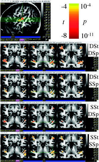
Intrablock repetition effect for the 4 stimulus conditions. The image on the top, left shows the location of the axial cut‐planes shown in the 4 panels below. Crosshairs are in the left STG at −55 [L], −21 [P], 4 [S] mm (TT‐Atlas), or −56 [L], −22 [P], 3 [S] mm (MNI‐Brain). Left BAs 41, 22, and 21 are within 2–4 mm from the focus point.

To determine if the trend was mostly due to the transition from silence to aural stimulation, the analysis was repeated using a narrower window, from 10 to 20 seconds. In that case, no significant trends were seen, even with lower thresholds. This suggests that the intrablock effect is driven mostly by the initial increased BOLD response, caused by the change from silence to auditory stimulation. In addition to the intrablock repetition effect, one can examine a consecutive‐sentence repetition effect by examining the response to same versus different sentences. We will examine this effect using the event‐related data next.

Group Analysis: Event Design

The event‐related design activated similar areas to the block design. All four stimulus classes activated overlapping areas that coincided with, but were smaller than, those shown in Figure 4. At the significance level of P < 0.05, corrected, we found one cluster in left middle temporal gyrus (MTG), BA 31, revealing a significant main effect for sentence. At a subthreshold level, a smaller cluster also appears in right MTG. No significant speaker effect was found, although at lower thresholds some effects were found colocalized with sentence effect areas. Consecutive‐sentence repetition effects were examined by contrasting different to same sentence (DSt vs. SSt) and different to same speaker. A cluster of voxels with significant difference between different and same sentence (DSt > SSt) was found in left MTG/inferior temporal gyrus (ITG) (BA 21). This cluster overlaps with the one showing sentence main effect. No significant effects were found for (DSP vs. SSp) at P < 0.05 corrected.

Significant interactions between sentence and speaker effect were found. The interactions were mostly caused by sentence effects with the same speaker: SSp (DSt vs. SSt). Table I lists the clusters showing interaction effects and Figure 6 shows, in the slice view, the location of the 3 clusters in the left hemisphere. Note that the clusters in bilateral middle temporal (BA 21/20) regions also showed significant activation relative to the control (silence) condition. However the cluster in inferior frontal region (BA 46/45) showed no significant activation relative to the rest condition. The 3‐D rendering shows the pattern of interaction in the entire brain. The viewpoint is from the left hemisphere and the crosshair, linked to the one in the sagittal slice, goes through the bilateral middle temporal clusters.

Table I.

Clusters of sentence and speaker interactions

Vol. μL	Center of mass (TT‐Atlas)	Location
3024	−59[L], −41[P], −1[I] mm	Left MTG, BA 21/22
1998	−54[L], 19[A], 12[S] mm	Left IFG, BA 44/45/46
1242	57[R], −7[P], −18[I] mm	Right MTG/ITG, BA 21/20
1053	−57[L], −11[P], −15[I] mm	Left MTG/ITG, BA 21/20

Figure 6.

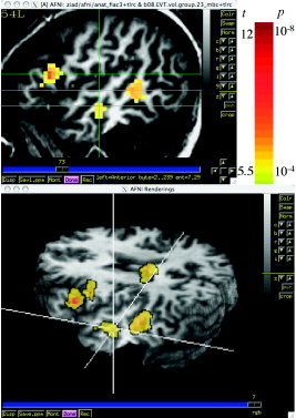
Areas showing interaction between sentence and speaker effects. The areas colored in red show significant effects for SSp (DSt > SSt). The slice view shows the location of the three clusters in the left hemisphere. The 3‐D rendering shows the pattern of interaction in the entire brain. The viewpoint is from the left hemisphere and the crosshair, linked to the one in the axial slice, and goes through the bilateral middle temporal clusters. In this view the color overlay “shines through” the brain, as if the brain were translucent. (Skull stripping was performed with the AFNI program 3dSkullStrip.) Talairach coordinates of the clusters' centers of mass are in Table I.

DISCUSSION

Prior work has shown that human voice perception and auditory sentence comprehension share several common regions of activity, including the bilateral STS/STG, MTG, and left inferior prefrontal region (Broca's area) [Belin et al., 2000; Fecteau et al., 2005]. The current design incorporates repetition conditions for both the speaker and sentence conditions. This manipulation allows for the dissociation of activation in regions based on biased processing of specific properties of either sentences or voices. Regions showing a main effect exclusively for one of the two factors are considered to perform factor‐related processing, whereas regions showing interaction effects represent components of a recollective memory processing system.

In both the event‐related and block designs, results were consistent with previous studies of auditory sentence comprehension and human voice perception [Dehaene‐Lambertz et al., 2006], showing bilateral activation of both the anterior and posterior STG, including Heschl's gyrus. Additionally, the STS, MTG, and IFG were active in these conditions. The main effects from our group analysis were consistent with those found by Dehaene‐Lambertz et al. [2006]. A main effect for sentence repetition, but not voice, showed greater activation in left anterior STS and MTG for novel sentences. This left‐lateralized effect suggests that these regions are involved in sentence processing, rather than voice perception or identification processing. No regions showed consecutive voice identity suppression. This negative result could imply that none of these regions are specific to voice identification, but may also reflect the decreased effect size due to the limited number of novel speakers (10) relative to the number of novel sentences (640). Because the voice identities are only truly novel the first time they are presented, consecutive voice identity suppression effects in the voice domain may have been limited by a floor effect. Another explanation for the lack of speaker effect might be the instructions to the subjects that they would be tested on the sentence content but not voice identity.

Two‐factor, within‐subject ANOVA also revealed significant subject by sentence interactions. Unlike Dehaene‐Lambertz et al. [2006], whose permutation tests revealed interaction in right MTG, the present analysis showed bilateral activation in anterior MTG, left posterior MTG, and left IFG.

The linear trend analysis revealed intrablock repetition suppression for both voice and sentence. However, when the analysis was restricted to the medial portion of the block the effect was greatly reduced. This suggests that the intrablock decrease is due to differences in the response to the first stimulus following a period of silence compared to the remaining sentences in the block. This is supported by the results shown in Figure 5, where blocks with novel speakers and sentences (DSt‐DSp) showed decreases comparable to or greater than conditions with stimulus repetition.

As can be seen in Figure 4, the simple effect for the DSt‐DSp condition showed activation limited to anterior STS and STG. All other conditions showed similar patterns of activation. Although these regions have been implicated in auditory sentence processing, other language processing areas were not found activated in these data. This may be the result of the small percentage of trials reserved for the passive baseline task. Additionally, Binder et al. [1999] and McKiernan et al. [2003] showed that passive baseline conditions (e.g., visual fixation or the absence of a control stimulus) limited the regions of activation in many typical language‐processing areas relative to a simple auditory perceptual decision task.

CONCLUSIONS

Consistent with Dehaene‐Lambertz et al. [2006], we found significant main effects for both voice and sentence repetitions. Significant interactions were found in the right MTG similar to that found by Dehaene‐Lambertz et al. [2006]. Additionally, we found interactions in left MTG and IFG. Trend analysis revealed intrablock decreases in the BOLD signal heavily weighted by changes in the initial portion of the block, even in block with neither voice or sentence repetitions.

With the data as given, we selected several reasonable analyses from the AFNI suite; in a sense, we are using the software to explore the data rather than to address any particular scientific question. We did not quantitatively compare the event‐related results to the block design results, partly because the two sets of tasks are not obviously comparable in a cognitive sense. We computed, but do not report here, the contrasts and interactions between different task classes in the block design; some of these are significant, but difficult to interpret in the absence of a guiding hypothesis and research program.

AFNI and SUMA are a flexible software package, fully open‐source, with the ability to display data and results in many ways, rapidly, interactively, and comprehensively. The package also has an extensive suite of time series analysis programs, and general 2‐D–4‐D data manipulation utilities. AFNI can acquire/display images from scanners in real time, and perform registration and activation calculations while an imaging run progresses. With the advent of the NIfTI‐1 format, AFNI can also easily interchange data files with many of the other software packages discussed in this issue.

REFERENCES

- Amunts K, Zilles K (2001): Advances in cytoarchitectonic mapping of the human cerebral cortex. Neuroimaging Clin N Am 11: 151–169. [PubMed] [Google Scholar]
- Argall BD, Saad ZS, Beauchamp MS (2006): Simplified intersubject averaging on the cortical surface using SUMA. Hum Brain Mapp 27: 14–27. [DOI] [PMC free article] [PubMed] [Google Scholar]
- Belin P, Zatorre RJ, Lafaille P, Ahad P, Pike B (2000): Voice‐selective areas in human auditory cortex. Nature 403: 309–312. [DOI] [PubMed] [Google Scholar]
- Binder JR, Frost JA, Hammeke TA, Bellgowan PS, Rao SM, Cox RW (1999): Conceptual processing during the conscious resting state. A functional MRI study. J Cogn Neurosci 11: 80–95. [DOI] [PubMed] [Google Scholar]
- Cox RW (1996): AFNI: software for analysis and visualization of functional magnetic resonance neuroimages. Comput Biomed Res 29: 162–173. [DOI] [PubMed] [Google Scholar]
- Cox RW, Hyde JS (1997): Software tools for analysis and visualization of fMRI data. NMR Biomed 10: 171–178. [DOI] [PubMed] [Google Scholar]
- Dale AM, Fischl B, Sereno MI (1999): Cortical surface‐based analysis. I. Segmentation and surface reconstruction. Neuroimage 9: 179–194. [DOI] [PubMed] [Google Scholar]
- Dehaene‐Lambertz G, Dehaene S, Anton JL, Campagne A, Ciuciu P, Dehaene GP, Denghien I, Jobert A, LeBihan D, Sigman M, Pallier C, Poline JB (2006): Functional segregation of cortical language areas by sentence repetition. Hum Brain Mapp. In press. [DOI] [PMC free article] [PubMed] [Google Scholar]
- Fecteau S, Armony JL, Joanette Y, Belin P (2005): Sensitivity to voice in human prefrontal cortex. J Neurophysiol 94: 2251–2254. [DOI] [PubMed] [Google Scholar]
- Fischl B, Sereno MI, Dale AM (1999a): Cortical surface‐based analysis. II. Inflation, flattening, and a surface‐based coordinate system. Neuroimage 9: 195–207. [DOI] [PubMed] [Google Scholar]
- Fischl B, Sereno MI, Tootell RB, Dale AM (1999b): High‐resolution intersubject averaging and a coordinate system for the cortical surface. Hum Brain Mapp 8: 272–284. [DOI] [PMC free article] [PubMed] [Google Scholar]
- Forman SD, Cohen JD, Fitzgerald M, Eddy WF, Mintun MA, Noll DC (1995): Improved assessment of significant activation in functional magnetic resonance imaging (fMRI): use of a cluster‐size threshold. Magn Reson Med 33: 636–647. [DOI] [PubMed] [Google Scholar]
- Lancaster JL, Woldorff MG, Parsons LM, Liotti M, Freitas CS, Rainey L, Kochunov PV, Nickerson D, Mikiten SA, Fox PT (2000): Automated Talairach atlas labels for functional brain mapping. Hum Brain Mapp 10: 120–131. [DOI] [PMC free article] [PubMed] [Google Scholar]
- McKiernan KA, Kaufman JN, Kucera‐Thompson J, Binder JR (2003): A parametric manipulation of factors affecting task‐induced deactivation in functional neuroimaging. J Cogn Neurosci 15: 394–408. [DOI] [PubMed] [Google Scholar]
- Saad ZS, Reynolds RC, Argall B, Japee S, Cox RW (2004): SUMA: an interface for surface‐based intra‐ and inter‐subject analysis with AFNI. Arlington, VA: IEEE; p 1510–1513. [Google Scholar]
- Talairach J, Tournoux P (1988): Co‐planar stereotaxic atlas of the human brain: an approach to medical cerebral imaging. Stuttgart: G. Thieme; Thieme Medical Publishers. [Google Scholar]
- Van Essen DC (2002): Windows on the brain: the emerging role of atlases and databases in neuroscience. Curr Opin Neurobiol 12: 574–579. [DOI] [PubMed] [Google Scholar]
- Van Essen DC (2005): A population‐average, landmark‐ and surface‐based (PALS) atlas of human cerebral cortex. Neuroimage 28: 635–662. [DOI] [PubMed] [Google Scholar]
- Zilles K, Schleicher A, Palomero‐Gallagher N, Amunts K (2002): Quantitative analysis of cyto‐ and receptor architecture of the human brain In: Mazziotta JC, Toga A, editors. Brain Mapping, the Methods. Amsterdam: Elsevier; p 573–602. [Google Scholar]