Comparison of different cortical connectivity estimators for high‐resolution EEG recordings

Abstract

The aim of this work is to characterize quantitatively the performance of a body of techniques in the frequency domain for the estimation of cortical connectivity from high‐resolution EEG recordings in different operative conditions commonly encountered in practice. Connectivity pattern estimators investigated are the Directed Transfer Function (DTF), its modification known as direct DTF (dDTF) and the Partial Directed Coherence (PDC). Predefined patterns of cortical connectivity were simulated and then retrieved by the application of the DTF, dDTF, and PDC methods. Signal‐to‐noise ratio (SNR) and length (LENGTH) of EEG epochs were studied as factors affecting the reconstruction of the imposed connectivity patterns. Reconstruction quality and error rate in estimated connectivity patterns were evaluated by means of some indexes of quality for the reconstructed connectivity pattern. The error functions were statistically analyzed with analysis of variance (ANOVA). The whole methodology was then applied to high‐resolution EEG data recorded during the well‐known Stroop paradigm. Simulations indicated that all three methods correctly estimated the simulated connectivity patterns under reasonable conditions. However, performance of the methods differed somewhat as a function of SNR and LENGTH factors. The methods were generally equivalent when applied to the Stroop data. In general, the amount of available EEG affected the accuracy of connectivity pattern estimations. Analysis of 27 s of nonconsecutive recordings with an SNR of 3 or more ensured that the connectivity pattern could be accurately recovered with an error below 7% for the PDC and 5% for the DTF. In conclusion, functional connectivity patterns of cortical activity can be effectively estimated under general conditions met in most EEG recordings by combining high‐resolution EEG techniques, linear inverse estimation of the cortical activity, and frequency domain multivariate methods such as PDC, DTF, and dDTF. Hum. Brain Mapp, 2007. © 2006 Wiley‐Liss, Inc.

INTRODUCTION

Neuroscience has recognized that the concept of brain connectivity (i.e., how cortical regions communicate) is central to understanding the organized behavior of cortical regions, beyond the simple mapping of their activity [Brovelli et al.,2004,2005; Horwitz,2003; Lee et al.,2003]. Cortical connectivity estimation aims at describing these interactions as connectivity patterns that represent the direction and strength of the information flow between cortical areas. To achieve this, several methods have been applied to both hemodynamic and electromagnetic data [Brovelli et al.,2004; Buchel and Friston,1997; Lee et al.,2003]. Although the terminology is as yet inconsistent, two main definitions of brain connectivity have been proposed: functional and effective connectivity [Friston,1994; Horwitz,2003]. Functional connectivity is defined as the temporal correlation between spatially remote neurophysiologic events, whereas effective connectivity is defined as the simplest brain circuit that would produce the same temporal relationship as observed experimentally between cortical sites. Thus, effective connectivity captures a putatively causal relationship. For functional connectivity, computational methods proposed to estimate how different brain areas are working together typically involve the estimation of covariance properties between the time series measured from the different spatial sites during motor and cognitive tasks studied by EEG, MEG, or functional MRI (fMRI) techniques.

Structural Equation Modeling (SEM) has been used in the past decade with hemodynamic and metabolic measurements to assess effective connectivity [Buchel and Friston,1997; McIntosh and Lima,1994]. The basic idea of SEM differs from the usual statistical approach of modeling individual observations, since SEM considers the covariance structure of the data. However, the estimation of cortical effective connectivity obtained with the application of the SEM technique to fMRI data has a low temporal resolution (on the order of several seconds), which is far slower than the time scale on which many brain events normally unfold. Such temporal resolution can be improved by applying the SEM to high‐resolution EEG data [Astolfi et al.,2005a].

One issue is that the SEM approach is model‐dependent, although in general a connectivity model is not available before the data analysis. Thus, data‐driven functional connectivity methods that do not need an a priori connectivity model would have considerable appeal. Among the linear and nonlinear methods used to estimate functional brain connectivity [Clifford Carter,1987; Gevins et al.,1989; Inouye et al.,1995; Nunez,1995; Stam and van Dijk,2002; Stam et al.,2003, Tononi et al.,1994; Urbano et al.,1998], frequency‐based methods are particularly attractive for the analysis of EEG or MEG data, since the activity of neural populations is often best expressed in this domain [Gross et al.,2001,2003; Pfurtscheller and Lopes da Silva,1999]. Many EEG and/or MEG frequency‐based methods that have been proposed in recent years for assessment of the directional influence of one signal on another are based mainly on the Granger [1969] theory of causality. Granger theory mathematically defines what is a “causal” relation between two signals. According to this theory, an observed time series x(n) is said to cause another series y(n) if the knowledge of x(n)'s past significantly improves prediction of y(n); this relation between time series is not necessarily reciprocal, i.e., x(n) may cause y(n) without y(n) causing x(n). This lack of reciprocity allows the evaluation of the direction of information flow between structures. Kaminski and Blinowska [1991; Kaminski et al.,2001] proposed a multivariate spectral measure, called the Directed Transfer Function (DTF), which can be used to determine the directional influences between any given pair of channels in a multivariate dataset. DTF is an estimator that simultaneously characterizes the direction and spectral properties of the interaction between brain signals and requires only one multivariate autoregressive (MVAR) model to be estimated simultaneously from all the time series. The advantages of MVAR modeling of multichannel EEG signals in order to compute efficient connectivity estimates have recently been stressed. Kus et al. [2004] demonstrated the superiority of MVAR multichannel modeling with respect to the pairwise autoregressive approach.

Another popular estimator, the Partial Directed Coherence (PDC), based on MVAR coefficients transformed into the frequency domain was recently proposed [Baccala and Sameshima,2001], as a factorization of the Partial Coherence. The PDC is of particular interest because of its ability to distinguish direct and indirect causality flows in the estimated connectivity pattern. As will be explained mathematically in the following paragraph, if a “true” causality flow exists linking the signals recorded from region A to region B, and if another “true” flow exists from region B to region C, the PDC estimator does not add an “erroneous” causality flow between the signal recorded from region A to region C. This property is particularly interesting in its application to brain signals, where the interpretation of a direct connection between two cortical regions is straightforward.

Over the last decade, a body of techniques known as high‐resolution EEG has allowed precise estimation of cortical activity from noninvasive EEG measurements [Gevins,1989; Gevins et al.,1991,1999; He and Lian,2002; He et al.,2002; Nunez,1995]. These methods involve the use of a large number of scalp electrodes or sensors, realistic models of the head derived from structural magnetic resonance images (MRIs), and advanced processing techniques related to the solution of the linear inverse problem, which enable the estimation of cortical current density from sensor measurements [Babiloni et al.,2000; Grave de Peralta and Gonzalez Andino,1999; Pascual‐Marqui,1995]. Previous simulation studies analyzed the ability of the DTF to recover the scalp and cortical connectivity from EEG signals [Astolfi et al.,2005b; Korzeniewska et al.,2003]. It has been recently pointed out that the DTF can recover cortical connectivity patterns under a large range of signal‐to‐noise ratios (SNRs) and recording lengths [Astolfi et al.,2005b]. However, the formulation of DTF makes it possible in certain conditions to derive an incorrect estimation of the paths between cortical areas. To improve the capability of DTF to detect direct and indirect causality pathways, Korzeniewska et al. [2003] introduced the direct DTF (dDTF) in order to deal with such pathways. It has been suggested that the use of PDC or dDTF techniques could overcome this drawback [Baccala and Sameshima,2001; Korzeniewska et al.,2003]. However, several questions related to the precision of the estimates of the connectivity patterns returned by DTF, PDC, and dDTF in conditions with different SNR and recording lengths remain unaddressed.

The present study focused on the following open questions:

• 1How are the connectivity pattern estimators DTF, PDC, and dDTF influenced by different factors affecting the EEG recordings, like the SNR and the amount of data available?
• 2How do the estimators perform in the discrimination of direct or indirect causality patterns?
• 3What is the most effective method for estimating a connectivity model under the conditions usually encountered in standard EEG recordings?

In the present study, these questions were addressed via simulations, using predefined connectivity schemes linking several cortical areas. Estimates of the cortical connections under different conditions were then retrieved using DTF, PDC, and dDTF methods. The results obtained for the different estimators were then statistically evaluated by analysis of variance (ANOVA). After characterizing the performance of the different connectivity estimators in the simulation study, their potential for the evaluation of brain connectivity is illustrated using high‐resolution EEG recorded during a standard Stroop task.

MATERIALS AND METHODS

Multivariate Methods for the Estimation of Connectivity

Let Y be a set of cortical waveforms, obtained from several cortical regions of interest (ROIs), as described in detail in the following paragraph:

(1)

where t refers to time and N is the number of cortical areas considered.

Supposing that the following MVAR process is an adequate description of the dataset Y:

(2)

where Y(t) is the data vector in time, E(t)=[e₁(t), …, e_N]^T is a vector of multivariate zero‐mean uncorrelated white noise processes, Λ(1), Λ(2), … Λ(p) are the N×N matrices of model coefficients and p is the model order. In the present study, p was chosen by means of the Akaike Information Criteria (AIC) for MVAR processes [Akaike,1974] and was used for MVAR model fitting to simulations, as well as to experimental signals. It has been noted that, although the sensitivity of MVAR performance depends on the model order, small model order changes do not influence results [Babiloni et al.,2005; Franaszczuk et al.,1985].

A modified procedure for the fitting of MVAR on multiple trials was adopted [Astolfi et al.,2005b; Babiloni et al.,2005; Ding et al.,2000]. When many realizations of the same stochastic process are available, as in the case of several trials of an event‐related potential (ERP) recording, the information from all the trials can be used to increase the reliability and statistical significance of the model parameters. In the present study, both in the simulation and in the application to real data, the data were in the form of several trials of the same length, as described in detail in the following sections.

Once an MVAR model is adequately estimated, it becomes the basis for subsequent spectral analysis. To investigate the spectral properties of the examined process, Eq. (2) is transformed to the frequency domain:

(3)

where:

(4)

and Δt is the temporal interval between two samples. Equation (3) can be rewritten as:

(5)

where H(f) is the transfer matrix of the system, whose element H_ij represents the connection between the j‐th input and the i‐th output of the system.

Directed Transfer Function

The DTF, representing the causal influence of the cortical waveform estimated in the j‐th ROI on that estimated in the i‐th ROI as defined [Kaminski and Blinoswka,1991] in terms of elements of the transfer matrix H, is:

(6)

In order to compare the results obtained for cortical waveforms with different power spectra, a normalization can be performed by dividing each estimated DTF by the squared sums of all elements of the relevant row, thus obtaining the so‐called normalized DTF [Kaminski and Blinoswka,1991]:

(7)

γ_ij(f) expresses the ratio of influence of the cortical waveform estimated in the j‐th ROI on the cortical waveform estimated in the i‐th ROI, with respect to the influence of all the estimated cortical waveforms. Normalized DTF values are in the interval [0, 1], and the normalization condition

(8)

is applied.

From the transfer matrix, we can calculate power spectra S(f). If we denote by V the variance matrix of the noise E(f), the power spectrum is defined by:

(9)

where the superscript * denotes transposition and complex conjugate.

From S(f), ordinary coherence can be computed as:

(10)

Coherence measures express the degree of synchrony (simultaneous activation) between areas i and j.

Partial Directed Coherence

Partial coherence is another estimator of the relationship between a pair of signals, describing the interaction between areas i and j when the influence due to all N‐2 time series is discounted. It is defined by the formula:

(11)

where M_ij(f) is the minor obtained by removing i‐th row and j‐th column from the spectral matrix S.

In 2001, Baccala proposed the following factorization:

(12)

where Λ_n (f) is the n‐th column of the matrix Λ (f). This led to the definition of PDC [Baccala,2001]:

(13)

The PDC from j to i, π_ij(f), describes the directional flow of information from the activity in the ROI s_j(n) to the activity in s_i(n), whereupon common effects produced by other ROIs s_k(n) on the latter are subtracted, leaving only a description that is specifically from s_j(n) to s_i(n).

PDC values are in the interval [0, 1], and the normalization condition:

(14)

is verified. According to this condition, π_ij(f) represents the fraction of the time evolution of ROI j directed to ROI i, compared to all of j's interactions with other ROIs.

For both DTF and PDC, high values in a frequency band represent the existence of an influence between any given pair of areas in the dataset. However, an important difference is that PDC does not involve the inversion of matrix Λ. This leads to several points. In fact, an analysis of the definition of DTF reveals that, due to this matrix inversion, it is a linear combination of both the direct influence from one area to the other and the influence mediated by other areas along various cascade pathways [Kaminski et al.,2001]. This becomes immediately clear from an example: given a three‐region model, the nonnormalized DTF from area 1 to area 2 is:

(15)

From this formula it can be noted that even if the direct influence from area 1 to area 2, Λ₂₁ (f), is zero, {9i}may still be different from zero, since there is an influence from 1 to 3 (Λ₃₁ (f)) and from 3 to 2 (Λ₂₃ (f)). The link between 1 and 2 will be indicated by DTF as a causal pathway if all the causal influences along the way are nonzero.

PDC, due to the lack of the matrix inversion, behaves differently. It indicates only the existence of a direct causal influence from area 1 to area 2. If no direct influence exists, PDC₂₁ is virtually zero.

Direct DTF

In order to distinguish between direct and cascade flows in DTF, the direct DTF (dDTF) was introduced [Korzeniewska et al.,2003]. It is defined by multiplying the full frequency DTF (ffDTF), given by:

(16)

by the partial coherence defined in Eq. 11. The dDTF from area j to area i is defined as:

(17)

This function describes only the direct relations between channels. The denominator of the ffDTF function (16) does not depend on frequency.

Simulation Study

The experimental design involved the following steps.

• 1Generation of a set of test signals simulating cortical average activations. Several sets of simulated data were generated in order to fit a predefined connectivity model and to respect imposed levels of the SNR (factor SNR) and the length of the data (factor LENGTH). The data were in the form of multiple trials, and the factor LENGTH indicates the total length of all trials.
• 2Estimation of the cortical connectivity pattern obtained under different conditions. The estimators used were DTF, PDC, and dDTF.
• 3Computation of indices of connectivity estimation performance. These indices were error functions describing the error in the connectivity estimation for the whole pattern and for each single arc. A comparison between the value estimated for the direct and indirect arcs was also performed.
• 4Statistical analysis (ANOVA) of the results of the simulations performed to study the effects of the factors SNR and LENGTH on the recovery of the connectivity pattern resulting from the different methods.

Signal Generation

The connectivity model used in the generation of test signals is shown in Figure 1A. It involves five areas, linked by both direct and indirect pathways. For example, ROIs 1 and 2 are linked by a direct path directed from 1 to 2. ROIs 1 and 5 are not connected by any direct arc but are linked by an indirect path, from 1 to 2 and from 2 to 5. ROIs 4 and 5 are not linked by either a direct or an indirect arc. As described above, these situations are rather different with respect to the estimates obtained by multivariate methods based on MVAR models. In particular, the model shown in Figure 1 has 7 direct arcs, 2 indirect arcs, and 11 “null” arcs (i.e., 11 pairs of ROIs are not linked, either directly or indirectly).

Figure 1.

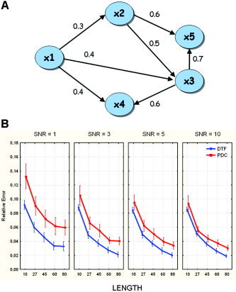
A: Connectivity model imposed in the generation of simulated signals. Values on the arrows represent the connection strengths. B: Results of the ANOVA performed on the relative error made in the estimation of the connectivity flows. The diagram shows the influence of the different levels of the main factors SNR and LENGTH on the estimation of the correct flows in the connection graph employed for the simulation for the two estimators DTF and PDC. The bar on each point represents the 95% confidence interval of the mean errors computed across the simulations. Duncan post‐hoc test (performed at 5%) showed no significant difference between levels 3, 5, and 10 of factor SNR. [Color figure can be viewed in the online issue, which is available at www.interscience.wiley.com.]

The simulated signals were obtained starting from a neural mass model of an ROI, fit to a real cortical estimation of the average activity in a ROI. Signal x₁ was a waveform generated by a model of three neural populations, arranged in parallel. Each population simulates neural activity in a specific frequency band: 4–12 Hz, 12–30 Hz, and 30–50 Hz. The model of each population is based on equations proposed by Wendling et al. [2002]. The basic idea behind this model is that oscillations derive from the interactions of pyramidal neurons with three other local neural subsets: excitatory interneurons, slow inhibitory interneurons, and fast inhibitory interneurons. Parameters of the three populations (time constants and synaptic gains) were set by using an automatic best‐fitting procedure to mimic the entire power spectrum density of cortical activity in an ROI.

Subsequent signals x₂(t) to x₅(t) were iteratively obtained according to the imposed connectivity scheme (Fig. 1A) by adding to signal x_j contributions from the other signals, delayed by intervals τ_ij and amplified by factors a_ij, plus uncorrelated Gaussian white noise. Coefficients of the connection strengths were chosen in a range of realistic values as observed in studies that applied other connectivity estimation techniques, like SEM, to several memory, motor, and sensory tasks [ Buchel and Friston,1997; Fa‐Hsuan,2003]. The values used for the connection strengths are given in the legend of Figure 1. The data were generated using different delay schemes on the connectivity pattern imposed. The values used for the delay from the i‐th ROI to the j‐th (τ_ij) ranged from 1 sample up to p‐2, where p was the order of the MVAR model used. These schemes were chosen in order to cover a variety of situations, to represent the effect of different delay conditions.

Generation of simulated data was repeated under the following combinations of conditions: SNR factor levels = [1, 3, 5, 10]; LENGTH factor levels = [2,500, 6,750, 11,250, 15,000, 20,000] data samples, corresponding to a signal length of [10, 27, 45, 60, 80] s, in the form of several trials of the same length, at a sampling rate of 250 Hz.

The levels chosen for both SNR and LENGTH factors cover a typical range for cortical activity estimated from ERPs with high‐resolution EEG techniques.

The MVAR model was estimated by means of the Nuttall‐Strand method, or multivariate Burg algorithm, which has been demonstrated to provide the most accurate results [Kay,1988; Marple,1987; Schlögl,2003].

Evaluation of Performance

A statistical evaluation of the performance of the different estimators required a precise definition of an error function, describing the goodness of the pattern recognition. This was achieved by focusing on the MVAR model structure described in Eq. 2 and comparing it to the signal generation scheme. The elements of matrices Λ(k) of MVAR model coefficients can be related to the coefficients used in the signal generation and are different from zero only for k = τ_ij, where τ_ij is the delay chosen for each pair ij of ROIs and for each direction among them. In particular, for the independent reference source waveform x₁(t), an autoregressive model of the same order of the MVAR was estimated, with coefficients a₁₁(1), …, a₁₁(p) corresponding to the elements Λ₁₁(1), …, Λ₁₁(p) of the MVAR coefficients matrix. Thus, with the estimation of the MVAR model parameters, we aimed to recover the original coefficients a_ij(k) used in signal generation. In this way, reference functions were computed for each of the estimators on the basis of the signal generation parameters. The error function was then computed as the difference between these reference functions and the estimated ones (both averaged in the frequency band of interest).

To evaluate the performance in retrieving connections between areas, we used the Frobenius norm of the matrix reporting the differences between the values of the estimated and the imposed connections (Relative Error):

(18)

where ζˆ _ij(f₁, f₂) is the mean value of the estimator function estimated in the frequency band (f_1,f₂), and ζ _ij(f₁,f₂) is the mean value of the reference functions obtained from the generation model in the same frequency band. Here, ζ _ij can be DTF or PDC.

Simulations were performed by repeating each generation‐estimation procedure 50 times in order to increase the robustness of the successive statistical analysis.

Statistical Analysis

The results obtained were subjected to separate ANOVA. The first analysis was a three‐way ANOVA examining the effect of SNR, LENGTH, and the different methods used to estimate the cortical connectivity (METHODS) on the error for the entire connectivity model estimated. The “within” main factors of the ANOVAs were SNR (with four levels: 1, 3, 5, 10), LENGTH (with six levels: [2,500, 6,750, 11,250, 15,000, 20,000] data samples, corresponding to a signals length of [10, 27, 45, 60, 80] s, in three trials of the same length, at a sampling rate of 250 Hz) and METHODS (with two levels: DTF and PDC). The dependent variable was the Relative Error defined in Eq. (18). The Greenhouse‐Geisser correction for the violation of the spherical hypothesis was used. Duncan post‐hoc analyses at P = 0.05 significance level were then performed.

As explained above, the presence of indirect paths in the network (i.e., a path linking a node to another node on the network not directly but through one or more intermediate nodes) is a critical situation for MVAR‐based estimators of causality relations. For this reason, particular attention was paid to the analysis of the estimation error in such indirect relationships. Another ANOVA was performed where the values estimated on the indirect arcs by the three methods, DTF, PDC, and dDTF, were compared to the average value of the parameters estimated on the arcs actually present in the generation model. The dependent variable was the absolute level of the connectivity estimates, while the independent factors were METHODS, LENGTH, SNR, and PATHS. The first three main factors had the same levels used before in the other ANOVAs, and the main factor PATHS had three levels, describing the value of the dependent variable for the “indirect” links moving from the area x₁to the area x₅, that from the area x₂ to the area x₄, and the average value estimated on nonzero arcs in the model. The Greenhouse‐Geisser correction was used also in this case.

Head and Cortical Models

In order to estimate cortical activity from actual EEG scalp recordings, realistic head models reconstructed from T1‐weighted MRIs were employed. Scalp, skull, and dura mater compartments were segmented from MRIs and tesselated with ∼5,000 triangles for each surface. A source model was built using the following procedure: 1) the cortex compartment was segmented from MRIs and tesselated to obtain a fine mesh with ∼100,000 triangles; 2) a coarser mesh was obtained by resampling the fine mesh down to ∼5,000 triangles (this was done by preserving the general features of the neocortical envelope, especially in correspondence with pre‐ and postcentral gyri and frontal mesial area); and 3) an orthogonal unitary equivalent current dipole was placed in each node of the tesselated surface, with the direction parallel to the vector sum of the normals to the surrounding triangles.

High‐Resolution EEG Recordings

High‐density EEG recordings were performed on a group of five normal subjects. Here we present the connectivity results related to one representative subject in order to illustrate the potential of the methods investigated. Subjects were seated in a comfortable chair in a quiet room connected to the adjacent equipment room by intercom. They viewed a screen where the name of a color (e.g., “red”) was printed in the same color (e.g., in red ink, congruent condition) or a different color (e.g., in blue ink, incongruent condition). Blocks of congruent or incongruent words alternated with blocks of neutral words (not color names). There were 256 trials in 16 blocks (four color congruent, eight neutral, four color‐incongruent) of 16 trials, with a variable intertrial interval averaging 2,000 ms between trial onsets. Within the congruent blocks, half of the words were neutral, to prevent the development of word‐reading strategies in the congruent blocks. A trial began with the presentation of a word for 1,500 ms, followed by a fixation cross for an average of 500 ms. Each trial consisted of one word presented in one of four ink colors (red, yellow, green, blue), with each color occurring equally often with each word type (congruent, neutral, incongruent). Subjects were asked to press one of four buttons that corresponded to the color of the ink of the presented word. Data from 0–450 ms poststimulus was analyzed.

EEG was recorded using well‐established methods (e.g., following the recent guidelines of Picton et al. [2002]). A custom‐designed Falk Minow cap located 64 scalp locations for EEG and EOG recording, with the EEG electrodes spaced equidistantly, with left mastoid serving as the reference for all other sites. Electrode impedances were below 10 K ohms. Amplifier bandpass was 0.1–100 Hz with digitization at 250 Hz, and the EEG data were successively digitally filtered at 50 Hz. Electrode positions were digitized using a Zebris 3D localization device with respect to anatomic landmarks (nasion and two preauricular points). ERP data were visually inspected and trials containing artifacts were rejected. A semiautomatic, supervised threshold criteria was used for the rejection of trials contaminated by ocular and EMG artifacts, as described in detail elsewhere [Moretti et al.,2003]. After artifact rejection, ERP signals were baseline adjusted.

Regions of Interest (ROIs)

Cortical ROIs were drawn by a neuroradiologist on the computer‐based cortical reconstruction of the individual head model of each subject. ROIs representing the left and right primary motor areas (MI) included Brodmann area 4 (BA 4). ROIs representing the supplementary motor area (SMA) were obtained from cortical voxels belonging to the more general BA 6. In particular, the posterior SMAp was depicted bilaterally on the medial frontal wall by following the anatomical landmarks recommended by Picard and Strick [1996]: the anterior border of the SMAp corresponded to a plane perpendicular to the anterior–posterior commissure (AC‐PC) line at the level of the AC (VAC), and a perpendicular plane at the level of the posterior commissure (VPC) represented the SMAp posterior border. ROIs from the right and left parietal areas including BA 7 and 5 were selected. In the frontal regions BAs 8 and 9/46 were selected. The cingulate (CMA) area (left and right) was also selected

Estimation of Cortical Source Current Density

The solution of the following linear system:

(19)

provides an estimation of the dipole source configuration x that generates the measured EEG potential distribution b. The system also includes the measurement noise n, assumed to be normally distributed. A is the lead field matrix, where each j‐th column describes the potential distribution generated on the scalp electrodes by the j‐th unitary dipole. The current density solution vector ζ of Eq. 10 was obtained as [Grave de Peralta and Gonzalez Andino,1999]:

(20)

where M, N are the matrices associated to the metrics of the data and of the source space, respectively, λ is the regularization parameter and ‖ x ‖_M represents the M norm of the vector x. The solution of Eq. (20) is given by the inverse operator G:

(21)

An optimal regularization of this linear system was obtained by the L‐curve approach [Hansen,1992a,b]. As a metric in the data space we used the identity matrix, while as a norm in the source space we use the following metric:

(22)

where (N ^‐1)_ii is the i‐th element of the inverse of the diagonal matrix N and all the other matrix elements N_ij are set to 0. The L₂ norm of the i‐th column of the lead field matrix A is denoted by ‖A _.i‖.

Cortical Estimated Waveforms

Using the relations described above, an estimate of the signed magnitude of the dipolar moment for each one of the 5,000 cortical dipoles was obtained for each timepoint. As the orientation of the dipole was defined to be perpendicular to the local cortical surface in the head model, the estimation process returned a scalar rather than a vector field. To obtain the cortical current waveforms for all the timepoints, we used a unique “quasi‐optimal” regularization λ value for all the analyzed EEG potential distributions. The quasi‐optimal regularization value was computed as an average of the several λ values obtained by solving the linear inverse problem for a series of EEG potential distributions. These distributions are characterized by an average Global Field Power (GFP) with respect to the higher and lower GFP values obtained from all the recorded waveforms. The instantaneous average of the signed magnitude of all the dipoles belonging to a particular ROI was used to estimate the average cortical activity in that ROI during the entire interval of the experimental task. These waveforms were then subjected to the MVAR estimation in order to estimate the connectivity pattern between ROIs. For a given ROI pair, the significance of the estimated cortical connectivity pattern was determined by comparison of its value to a threshold level. To estimate the thresholds for the functions values indicating lack of transmission, a surrogate data generation procedure was performed [Astolfi et al.,2005b]. The time series data from each ROI were randomly shuffled in order to remove interactions between signals. The connectivity estimators were then computed on these surrogate data. The procedure was repeated 1,000 times and an empirical distribution was generated. The significance threshold was set at 0.01. Only values beyond this threshold were considered to indicate the existence of a connection between each pair of ROIs.

Connectivity Pattern Representation

The connectivity patterns are represented by arrows pointing from one cortical area (“the source”) toward another one (“the target”). The arrow's color and size code the strength of the functional connectivity estimated between the source and the target. The bigger and the lighter the arrow, the stronger the connection. Only the cortical connections statistically significant at P < 0.01 are represented, according to the thresholds obtained, as previously described.

The connectivity patterns in the different frequency bands (Theta, 4–8 Hz; Alpha, 8–12 Hz; Beta, 13–30 Hz; Gamma, 30–40 Hz) between the different cortical regions were summarized by using indices representing the total flow from and toward the selected cortical area. The total inflow in a particular cortical region was defined as the sum of the statistically significant connections from all the other cortical regions toward the selected area. The total inflow for each ROI is represented by a sphere centered on the cortical region whose radius is linearly related to the magnitude of all the incoming statistically significant links from the other regions. Inflow information is also coded through a color scale. This information depicts each ROI as the target of functional connections from the other ROIs. The same conventions were used to represent the total outflow from a cortical region, generated by the sum of all the statistically significant links obtained by the application of the DTF to the cortical waveforms.

RESULTS

Simulation Study

Several sets of signals were generated as described in the previous section in order to fit a predefined connectivity pattern involving five cortical areas (shown in Fig. 1A). The graph depicts the flow of information from area x₁ toward areas x₂‐x₅. This connectivity model contains two indirect paths, where the signal is transmitted to a destination by only indirect relationships and with no direct link between the source area and the target one (from area x₂ to area x₄ through x₃, and from area x₁ to area x₅ through x₂ and x₃, with several different paths: x1→x3→x5 and x1→x2→x3→x5).

A multivariate autoregressive model of order 10 was fitted to each set of simulated data, which were in the form of about 30 trials of the same length. The procedure of signal generation and connectivity estimation for the different methods was carried out 50 times for each level of the factors SNR and LENGTH to increase the robustness of the subsequent statistical analysis. The index of performance, i.e., the Relative Error, Eq. (12), and the estimated value on direct/indirect arcs were computed for each generation‐estimation procedure and then subjected to two ANOVAs.

In the first ANOVA the dependent variable was the Relative Error, representing the average error for the entire connectivity pattern estimated. Results revealed a strong influence of the main factors SNR (F = 205, P < 0. 0001), METHODS (F = 1190, P < 0. 0001), and LENGTH (F = 1644, P < 0. 0001), as well as the SNR × METHOD interaction (F = 56, P < 0. 0001) on the Relative Error. Figure 1B shows the influence of the levels of the main factors LENGTH and SNR on the Relative Error in the entire connectivity graph for each estimator. The errors resulting from DTF, evaluated with respect to the theoretical values that represent the ideal information obtainable by this indicator, were smaller than those resulting from PDC for every level of SNR and LENGTH. This indicates that DTF is more robust with respect to noise and amount of data available for its estimation. In particular, Figure 1B shows that for each increase in length of the recordings, there is a constant decrease in estimation error. The influence of the factor SNR is weaker. Post‐hoc tests revealed that there were no significant differences between levels 3, 5, and 10 of the SNR factor. The bar on each point represents the 95% confidence interval of the mean errors computed across the simulations.

Particular attention was paid to the ability of the different estimators to distinguish between direct and indirect causality flows. The values estimated for the two indirect pathways in the model were compared to the average value obtained for the direct arcs present in the connectivity model imposed. The values of the connections imposed between cortical areas ranged from 0.3–0.7. The two indirect paths analyzed were arc 1→5 and arc 2→4, indicated by the large arrows in Figure 2A. As expected, DTF was not always able to attribute a zero value to a nondirect arc. On the other hand, PDC and dDTF correctly recognized the indirect path in all cases, estimating values close to zero in these instances (see Fig. 2B). However, the results obtained by dDTF for the direct arcs were also very small if compared to the other methods. Post‐hoc tests revealed no differences between values obtained by dDTF on the average of direct arcs and the values obtained by the same method on indirect arcs. The ANOVA revealed a strong influence of the main factors SNR (F = 20, P < 0,0001), METHOD (F = 2980000, P < 0,0001), and LENGTH (F = 493, P < 0,0001). Furthermore, all possible interactions of the main factors were significant, with F values not below 3 and P always below 0.001.

Figure 2.

A: Connectivity model imposed on the simulated signals. The thick arrows represent the indirect pathways linking the cortical areas. B: Average connectivity values estimated on two indirect links (1→5 and 2→4) and for all the other existing arcs for the networks by the three methods DTF, PDC, and dDTF during all the simulations. [Color figure can be viewed in the online issue, which is available at www.interscience.wiley.com.]

Application to Real High‐Density EEG Data

After the solution of the linear inverse problem, the estimation of the current density waveforms on each ROI was obtained as described in Materials and Methods. Connectivity estimations were performed by DTF, PDC, and dDTF, and the statistical thresholds were evaluated via the shuffling procedure previously described. The order of the MVAR model used for each estimation was determined by means of the Akaike Information Criterion (AIC), which returned an optimal order of 13. Details of the electrode montage are shown on the realistic reconstruction of a subject's scalp in Figure 3. The different ROIs selected are shown in different colors on the realistic reconstruction of the subject's left cortical hemisphere (regions of the cortex not of interest are shown in gray). By means of the linear inverse procedure, the estimation of the current density waveforms in each ROI was then performed according to Eqs. (19), (20), (21), (22). The DTF, PDC, and dDTF estimators were applied to the cortical waveforms related to the ROIs.

Figure 3.

Over the right hemisphere the electrode montage (59 electrodes) is shown on the realistic reconstruction of a subject's scalp, obtained from structural MRIs. Over the left hemisphere the ROIs considered for this study are shown on the realistic reconstruction of the subject's cortex. Each ROI is represented in a different color. The ROIs considered are the cingulate motor area (CMA), Brodmann areas 7 (A7) and 5 (A5), the primary motor area the posterior supplementary motor area (SMAp) and the lateral supplementary motor area (A6_L). [Color figure can be viewed in the online issue, which is available at www.interscience.wiley.com.]

Figure 4 shows the cortical connectivity patterns obtained for the CONGRUENT stimuli during the period preceding the subject's answer (0–450 ms after the stimulus presentation) in the representative subject. The results are shown for the beta band (12–29 Hz). The DTF (left), PDC (center), and dDTF (right) methods produced similar results. In particular, functional connections between cortical parietofrontal areas were present in all the estimations performed by the DTF, PDC, and dDTF methods. Moreover, connections involving the cingulate cortex are also clearly visible, as well as those involving prefrontal areas, mainly in the right hemisphere. Functional connections in prefrontal and premotor areas tended to be right‐sided, whereas the functional activity in the parietal cortices was generally bilateral.

Figure 4.

Cortical connectivity patterns obtained for the period preceding the subject's response during congruent trials in the beta (12–29 Hz) frequency band in a representative subject. The patterns are shown on the realistic head model and cortical envelope of the subject, obtained from sequential MRIs. The brain is seen from above, left hemisphere represented on the right side. Functional connections are represented with arrows that move from a cortical area toward another one. The arrows' colors and sizes code the strengths of the connections. The lighter and the bigger the arrows, the stronger the connections. Three connectivity patterns are depicted, estimated in the beta frequency band for the same subject with the DTF (left), the PDC (middle), and the dDTF (right). Only the cortical connections statistically significant at P < 0.01 are reported. [Color figure can be viewed in the online issue, which is available at www.interscience.wiley.com.]

Figure 5 shows the inflow (first row) and outflow (second row) patterns computed for the same subject in the beta frequency band, for the same time period shown in Figure 4. The ROIs that are very active as source or sink (i.e., the source/target of the information flow to/from other ROIs) show results that are generally stable across the different estimators. Values in the left column are related to the inflow and outflow computations obtained with the DTF methods, the central column is related to the flows obtained with the PDC, and the right column to the dDTF. Across methods, greater involvement of the right premotor and prefrontal regions is observed..

Figure 5.

The inflow (first row) and the outflow (second row) patterns obtained for the beta frequency band from each ROI during the congruent trials. The brain is seen from above, left hemisphere represented on the right side. In the first row the figure summarizes in red hues the behavior of an ROI in terms of reception of information flow from other ROIs, by adding the values of the links arriving on the particular ROI from all the others. The information is coded with the size and the color of a sphere centered on the particular ROI analyzed. The larger the sphere, the higher the value of inflow or outflow for any given ROI. In the second row the blue hues code the outflow of information from a single ROI towards all the others. [Color figure can be viewed in the online issue, which is available at www.interscience.wiley.com.]

DISCUSSION

Methodological Considerations

The present study examined the performance of three different techniques commonly used to assess information flows between scalp electrodes and local field potentials [Baccala and Sameshima,2001; Kaminski et al.,2001; Korzeniewska et al.,2003] on simulated and real cortical waveforms obtained via the linear inverse problem solution using the realistic head volume conductor models and high‐density EEG recordings. The spatial resolution provided by the techniques presented here has been previously characterized in a series of simulation studies using the present ROI analysis approach [Babiloni et al.,2000,2001,2003,2004]. The simulation studies involved realistic head models, high‐density EEG and MEG setups (with 64 and 128 electrodes as well as 143 magnetic sensors), and standard levels of SNRs (1, 3, 5, 10, 100). The returned errors are lower than 5% for the estimation of the shape (via the Cross‐Correlation measure) and energy (via the Relative Error measure) of the simulated cortical waveforms. These figures ensure that the estimation of the cortical current density by using high spatial sampling and realistic head models is a reliable process that allows a precise reconstruction of the cortical waveforms in a variety of experimental situations.

All the techniques investigated in the present study are based on the Granger theory and MVAR models. The approach using the DTF, PDC, and dDTF techniques has the advantage of providing connectivity links that can be interpreted in the sense of Granger causality, which includes a concept of directionality. Other techniques have been presented in the literature for the evaluation of functional connectivity of EEG/MEG data. For instance, the technique called Dynamic Imaging of Coherent Sources (DICS) [Gross et al.,2001,2003], which uses a spatial filter and a realistic head model, has been recently introduced and employed to assess connectivity between cortical areas from MEG data [Gross et al.,2001,2003; Pollock et al.,2005a,b]. This technique has the advantage, when compared to the DTF, PDC, and dDTF methods investigated here, of a direct mathematical characterization of its spatial resolution of the point spread function [Gross et al.,2003]. However, spectral coherence or DICS techniques do not return directly the direction of the flow between cortical areas, although in the latter case DICS is usually coupled with another technique able to estimate such directional flow, like the Directionality Index [Rosenblum and Pikovsky,2001]. A main difference between DICS and the approach presented here is in the estimation of cortical activity; specifically, the fact that the DICS technique is a beamformer [Huang et al.,2004]. Differences in the performance of beamformers and weighted minimum norm linear inverse techniques depend on the particular experimental setup used. In particular, it has been shown in simulation studies that EEG/MEG beamformers can reconstruct rather precisely the spatial location and the time series of neuronal sources when they exhibit a transient correlation in time [Hadjipapas et al.,2005]. On the other hand, if the correlation between source activities exceeds 30–40% of the total duration of the period over which the beamformer weights are computed, effects of temporal distortion and signal cancellation will be observed [Gross et al.,2001; Sekihara et al.,2002; VanVeen et al.,1997]. This suggests that, if the beamformer is obtained using covariance time windows that are long enough with respect to the duration of transient linear interaction between sources, it will return an accurate estimate of spatiotemporal source activity. However, if the covariance windows are sufficiently long, the portion of the stimulus will be small in comparison with the baseline state, and a decrease in the SNR will occur. This would ultimately result in a loss of spatial resolution [Gross et al.,2001; VanVeen et al.,1997].

An interesting issue is related to the possibility of applying the connectivity estimators to multimodal neuroelectric and hemodynamic data (i.e., from EEG/MEG and fMRI measurements). Recent simulation and experimental studies [Babiloni et al.,2003,2005; Dale et al., 2000; Liu et al.,1998] stated that the multimodal integration of EEG, MEG, and fMRI improves the quality of the cortical estimation when compared to any single modality alone. This was obtained by using MEG and fMRI estimation [Dale et al., 2000; Liu et al.,1998], EEG and fMRI [Babiloni et al.,2003,2005], or EEG and MEG [Babiloni et al.,2001,2004]. It is reasonable to expect that, with the improvement of the quality of the cortical estimation given by multimodal integration, the estimation of connectivity could improve as well. However, the effect of multimodal integration in terms of connectivity is not yet addressed in the literature, due to the lack of a precise model of electrovascular coupling. It is also worth noting that all the techniques (EEG, MEG, and fMRI) can detect the activity of a particular set of neural sources and are blind to others. For instance, the activity of stellate neurons in the cortex can be detected by the fMRI, because of their metabolic demand, but not by neuroelectromagnetic measurements, to which they are invisible due to the closed field they generate. On the other hand, transient (milliseconds) synchronous activity of a small subset of neurons can be detected by EEG and MEG but is invisible to fMRI [Nunez,1995]. Hence, the use of multimodal integration can provide information about cortical activity that moves beyond that offered by a single technique. This is an important point in favor of multimodal integration of EEG, MEG, and fMRI also in the perspective of the estimation of functional cortical connectivity.

Simulations

We performed a series of simulations to evaluate the use of connectivity estimators on test signals generated to simulate the average electrical activity of cerebral cortical regions, as it can be estimated from high‐resolution EEG recordings gathered under different conditions of noise and length of the recordings. The information on performance, limits of applicability, and range of errors under different levels of the several factors that are of interest in normal EEG recordings were inferred from statistical analysis (ANOVA and Duncan post‐hoc tests on the Relative and the single arc Error). The values used for the strength coefficients in simulations are consistent with the ones estimated in previous studies of a large sample of subjects performing memory, motor, and sensory tasks [Buchel and Friston,1997; Fa‐Hsuan,2003].

The simulations provided the following answers to the questions raised in the Introduction:

• 1Decreased SNR impairs the accuracy of the connectivity pattern estimation obtained by the DTF, PDC, and dDTF estimators.
• 2The length of the EEG recordings has a reliable effect on the accuracy of connectivity pattern estimations. A length corresponding to 27 s of nonconsecutive recordings with an SNR of at least 3 ensures that connectivity patterns can be accurately recovered with an error below 7% for PDC and 5% for DTF.
• 3The error variance observed for the DTF estimator is lower than that for PDC or dDTF. However, DTF has the highest bias in the estimate of the connectivity pattern, as it includes values for the indirect paths that were not generated in the simulations. It has been noted that there is a higher bias for dDTF than for PDC, since the first estimator often removes from the estimated connectivity pattern some direct paths that were present in the original modeling. In this respect, PDC is characterized by lower bias in the estimation of connectivity patterns under the present conditions of SNR and LENGTH.

In conclusion, the results indicate a clear influence of different levels of SNR and LENGTH on the efficacy of the estimation of cortical connectivity in each of the methods. In particular, it has been noted that an SNR equal or greater than 3 and an overall LENGTH of the estimated cortical data of 6,750 data samples (27 s at 250 Hz), even in several short trials, are sufficient to significantly decrease the errors on the indices of quality adopted in this study. These conditions are common in recordings of event‐related activity in humans. These recordings are usually characterized by SNRs ranging from 3 (movement‐related potentials) to 10 (sensory evoked potentials) [Regan et al.,1989].

The present simulations allowed an evaluation of the level of error expected for different arcs, related to direct or indirect pathways. In addition, comparisons were done between the relative errors obtained on single arcs characterized by only direct connections and those related to multiple paths between the source and the target. The results showed that the error was generally greater when the signal was transmitted to a destination by more than one path. This result (not presented here) is in agreement with the results of the study on indirect paths, according to which such transmission may induce an error in the MVAR estimation.

An ANOVA was also performed on the error values obtained for different delay schemes imposed during the signal generation, chosen in order to cover a variety of situations. The ANOVA results indicated that there was no significant influence of the delay on the performances of the methods.

The information obtained from the simulations was used to evaluate the applicability of these methods to actual event‐related recordings. The ERP signals, from a Stroop task, showed an SNR between 3 and 5 in the five subjects examined. Therefore, according to the simulation results, a small amount of error in the estimation of cortical connectivity patterns was expected.

All three estimators provided directional information (i.e., each of them allowed establishment of the direction of the information flow between two cortical areas) and directed information (i.e., they discriminated between direct and indirect connection paths). This information is not available using other techniques to assess coupling between signals, such as standard coherence (which lacks directionality). An evaluation of several methods for the computation of the functional connectivity between EEG/MEG signals was recently performed [David et al.,2004]. It was concluded that, although nonlinear methods, such as mutual information, nonlinear correlation, and generalized synchronization [Roulston,1999; Stam and van Dijk,2002; Stam et al.,2003], might be preferred when studying EEG broadband signals that are sensitive to dynamic coupling and nonlinear interactions expressed over many frequencies, the linear measurements (like those presented here) afford a rapid and straightforward characterization of functional connectivity.

Application to Real ERP Data

Although presented here only to demonstrate the capabilities of the estimation procedures with real data, the physiological results shown for a representative subject are consistent with those present in the Stroop literature. The Stroop task is often employed in studies of selective attention and has been found to be sensitive to prefrontal damage. For incongruent stimuli, PET and fMRI studies have shown activation of a network of anterior brain regions. Most studies report activation of the anterior cingulate cortex (ACC) and frontal polar cortex, and several authors have hinted at changes in regional cerebral blood flow (rCFB) in posterior cingulate and other posterior regions [Bench et al.,1993; Carter et al.,1995; Milham et al.,2003].

In the present study, ACC was approximately modeled by the CMA ROI and dorsolateral prefrontal areas by the 9/46 ROI. Connectivity analysis indicated intense, bilateral ACC activity during the task. The number of directed interactions was similar across several frequency bands, but there were differences in the connectivity structure across the congruent–incongruent tasks (not shown here). These results were corroborated by the inflow–outflow analysis that showed agreement between the methodologies used for the derivation of the connectivity patterns. The predominance of outflow from right premotor and prefrontal cortical areas is of interest, and the increased activity in the prefrontal cortical regions is in agreement with previous scalp observations. In an EEG Stroop study, West and Bell [1997] reported increased spectral power at medial (F3, F4) and lateral (F7, F8) frontal sites, as well as over parietal regions (P3, P4). They suggested that activation of the parietal cortex resulted from interaction between prefrontal and parietal regions during the suppression of the influence of the irrelevant word meaning. Interaction between parietal and frontal sites has been advocated as an explanation for the activation of posterior areas [Carter et al.,1995; Milham et al.,2003; West and Bell,1997]. Possibly, the minimization of the influence of irrelevant word information prompts directed interactions from parietal toward frontal sites.

In a previous coherence study [Schack et al.,1999], increased coherence between parietal and frontal sites was observed late in the trial. This behavior is not detectable at the scalp level. With the application of advanced high‐resolution EEG methodologies, including realistic cortical modeling, solution of the linear inverse problem, and the application to the computed cortical signals of connectivity pattern estimators, it became observable. These data suggest that cognitive control is implemented by medial and lateral prefrontal cortices that bias processes in regions that have been implicated in high‐level perceptual and motor processes [Egner and Hirsh,2005]. It is also striking that in all the frequency bands and for the five subjects analyzed the differences between the estimated connectivity patterns with the connectivity estimation methods were negligible (results not shown here). This result suggests that in practical conditions constant differences of only a few percent observed in the simulation studies between DTF, PDC, and dDTF estimators are not as significant as other factors such as SNR and recording LENGTH.

CONCLUSIONS

The results provided by the present simulation study suggest that, under conditions frequently met in the ERP literature (SNR of at least 3 and a total length over trials of the recorded ERP greater than 27 s), the estimation of functional connectivity by the DTF, PDC, and dDTF methods can be performed with only moderate quantitative errors. The use of high‐density ERP recordings and the estimation of the cortical waveforms in ROIs allows the evaluation of the functional cortical connectivity patterns during the Stroop task. These computational tools (high‐density EEG, estimation of cortical activity via linear inverse problem, DTF, PDC, and dDTF) can be of considerable value for assessing functional connectivity patterns from noninvasive EEG recordings in humans.

REFERENCES

- Akaike H (1974): A new look at statistical model identification. IEEE Trans Automat Control AC‐ 19: 716–723. [Google Scholar]
- Astolfi L, Cincotti F, Babiloni C, Carducci F, Basilisco A, Rossini PM, Salinari S, Mattia D, Cerutti S, Ben Dayan D, Ding L, Ni Y, He B, Babiloni F (2005a): Estimation of the cortical connectivity by high‐resolution EEG and structural equation modeling: simulations and application to finger tapping data. IEEE Trans Biomed Eng 52: 757–768. [DOI] [PubMed] [Google Scholar]
- Astolfi L, Cincotti F, Mattia D, Babiloni C, Carducci F, Basilisco A, Rossini PM, Salinari S, Ding L, Ni Y, He B, Babiloni F (2005b): Assessing cortical functional connectivity by linear inverse estimation and directed transfer function: simulations and application to real data. Clin Neurophysiol 116: 920–932. [DOI] [PubMed] [Google Scholar]
- Babiloni F, Babiloni C, Locche L, Cincotti F, Rossini PM, Carducci F (2000): High‐resolution electroencephalogram: source estimates of Laplacian‐transformed somatosensory‐evoked potentials using a realistic subject head model constructed from magnetic resonance images. Med Biol Eng Comput 38: 512–519. [DOI] [PubMed] [Google Scholar]
- Babiloni F, Carducci F, Cincotti F, Del Gratta C, Pizzella V, Romani GL, Rossini PM, Tecchio F, Babiloni C (2001): Linear inverse source estimate of combined EEG and MEG data related to voluntary movements. Hum Brain Mapp 14: 197–209. [DOI] [PMC free article] [PubMed] [Google Scholar]
- Babiloni F, Babiloni C, Carducci F, Romani GL, Rossini PM, Angelone LM, Cincotti F (2003): Multimodal integration of high‐resolution EEG and functional magnetic resonance imaging data: a simulation study. Neuroimage 19: 1–15. [DOI] [PubMed] [Google Scholar]
- Babiloni F, Babiloni C, Carducci F, Romani GL, Rossini PM, Angelone LM, Cincotti F (2004): Multimodal integration of EEG and MEG data: a simulation study with variable signal‐to‐noise ratio and number of sensors. Hum Brain Mapp 22: 52–62. [DOI] [PMC free article] [PubMed] [Google Scholar]
- Babiloni F, Cincotti F, Babiloni C, Carducci F, Basilisco A, Rossini PM, Mattia D, Astolfi L, Ding L, Ni Y, Cheng K, Christine K, Sweeney J, He B (2005): Estimation of the cortical functional connectivity with the multimodal integration of high‐resolution EEG and fMRI data by directed transfer function. Neuroimage 24: 118–131. [DOI] [PubMed] [Google Scholar]
- Baccala LA (2001): On the efficient computation of partial coherence from multivariate autoregressive model In: Callaos N, Rosario D, Sanches B, editors. Proceed 5th World Conf Cybernetics Systemics Informatics SCI. Orlando, FL. [Google Scholar]
- Baccala LA, Sameshima K (2001): Partial directed coherence: a new concept in neural structure determination. Biol Cybern 84: 463–474. [DOI] [PubMed] [Google Scholar]
- Bench CJ, Frith CD, Grasby PM, Friston KJ, Paulesu E, Frackowiak RSJ, Dolan RJ (1993): Investigations of the functional anatomy of attention using the Stroop test. Neuropsychology 31: 907–922. [DOI] [PubMed] [Google Scholar]
- Brovelli A, Ding M, Ledberg A, Chen Y, Nakamura R, Bressler SL (2004): Beta oscillations in a large‐scale sensorimotor cortical network: directional influences revealed by Granger causality. Proc Natl Acad Sci U S A 101: 9849–9854. [DOI] [PMC free article] [PubMed] [Google Scholar]
- Brovelli A, Lachaux JP, Kahane P, Boussaoud D (2005): High gamma frequency oscillatory activity dissociates attention from intention in the human premotor cortex. Neuroimage 28: 154–164. [DOI] [PubMed] [Google Scholar]
- Buchel C, Friston KJ (1997): Modulation of connectivity in visual pathways by attention: cortical interactions evaluated with structural equation modeling and fMRI. Cereb Cortex 7: 768–778. [DOI] [PubMed] [Google Scholar]
- Carter CS, Mintun M, Cohen JD (1995): Interference and facilitation effects during selective attention: an H215O PET study of Stroop task performance. Neuroimage 2: 264–272. [DOI] [PubMed] [Google Scholar]
- Clifford Carter G (1987): Coherence and time delay estimation. Proc IEEE 75: 236–255. [Google Scholar]
- David O, Cosmelli D, Friston KJ (2004): Evaluation of different measures of functional connectivity using a neural mass model. Neuroimage 21: 659–673. [DOI] [PubMed] [Google Scholar]
- Ding M, Bressler SL, Yang W, Liang H (2000): Short‐window spectral analysis of cortical event related potentials by adaptive multivariate autoregressive modeling: data preprocessing, model validation and variability assessment. Biol Cybern 83: 35–45. [DOI] [PubMed] [Google Scholar]
- Egner T, Hirsh J (2005): The neural correlates and functional integration of cognitive control in a Stroop task. Neuroimage 23: 539–547. [DOI] [PubMed] [Google Scholar]
- Fa‐Hsuan L (2003): Spatio temporal brain imaging and modeling. PhD thesis, Cambridge, MA: MIT Press.
- Franaszczuk PJ, Blinowska KJ, Kowalczyk M (1985): The application of parametric multichannel spectral estimates in the study of electrical brain activity. Biol Cybern 51: 239–247. [DOI] [PubMed] [Google Scholar]
- Friston KJ (1994): Functional and effective connectivity in neuroimaging: a synthesis. Hum Brain Mapp 2: 56–78. [Google Scholar]
- Gevins AS, Cutillo BA, Bressler SL, Morgan NH, White RM, Illes J, Greer DS (1989): Event‐related covariances during a bimanual visuomotor task. II. Preparation and feedback. Electroencephalogr Clin Neurophysiol 74: 147–160. [DOI] [PubMed] [Google Scholar]
- Gevins A, Brickett P, Reutter B, Desmond J (1991): Seeing through the skull: advanced EEGs use MRIs to accurately measure cortical activity from the scalp. Brain Topogr 4: 125–131. [DOI] [PubMed] [Google Scholar]
- Gevins A, Le J, Leong H, McEvoy LK, Smith ME (1999): Deblurring. J Clin Neurophysiol 16: 204–213. [DOI] [PubMed] [Google Scholar]
- Granger CWJ (1969): Investigating causal relations by econometric models and cross‐spectral methods. Econometrica 37: 424–438. [Google Scholar]
- Grave de Peralta Menendez R, Gonzalez Andino SL (1999): Distributed source models: standard solutions and new developments In: Uhl C, editor. Analysis of neurophysiological brain functioning. Berlin: Springer; p 176–201. [Google Scholar]
- Gross J, Kujala J, Hämäläinen M, Timmermann L, Schnitzler A, Salmelin R (2001): Dynamic imaging of coherent sources: studying neural interactions in the human brain. Proc Natl Acad Sci U S A 98: 694–699. [DOI] [PMC free article] [PubMed] [Google Scholar]
- Gross J, Timmermann L, Kujala J, Salmelin R, Schnitzler A (2003): Properties of MEG tomographic maps obtained with spatial filtering. Neuroimage 19: 1329–1336. [DOI] [PubMed] [Google Scholar]
- Hadjipapas A, Hillebrand A, Holliday IE, Singh KD, Barnes GR (2005): Assessing interactions of linear and nonlinear neuronal sources using MEG beamformers: a proof of concept. Clin Neurophysiol 116: 1300–1313. [DOI] [PubMed] [Google Scholar]
- Hansen PC (1992a): Analysis of discrete ill‐posed problems by means of the L‐curve. SIAM Rev 34: 561–580. [Google Scholar]
- Hansen PC (1992b): Numerical tools for the analysis and solution of Fredholm integral equations of the first kind. Inverse Problems 8: 849–872. [Google Scholar]
- He B, Lian J (2002): Spatio‐temporal functional neuroimaging of brain electric activity. Crit Rev Biomed Eng 30: 283–306. [DOI] [PubMed] [Google Scholar]
- He B, Zhang Z, Lian J, Sasaki H, Wu S, Towle VL (2002): Boundary element method based cortical potential imaging of somatosensory evoked potentials using subjects' magnetic resonance images. Neuroimage 16: 564–576. [DOI] [PubMed] [Google Scholar]
- Horwitz B (2003): The elusive concept of brain connectivity. Neuroimage 19: 466–470. [DOI] [PubMed] [Google Scholar]
- Huang MX, Shih J, Lee RR, Harrington DL, Thoma RJ, Weisend MP, Hanlon FM, Paulson KM, Li T, Martin K, Miller GA, Cañive JM (2004): Commonalities and differences among vectorized beamformers in electromagnetic source imaging. Brain Topogr 16: 139–158. [DOI] [PubMed] [Google Scholar]
- Inouye T, Iyama A, Shinosaki K, Toi S, Matsumoto Y (1995): Inter‐site EEG relationships before widespread epileptiform discharges. Int J Neurosci 82: 143–153. [DOI] [PubMed] [Google Scholar]
- Kaminski M, Blinowska K (1991): A new method of the description of the information flow in the brain structures. Biol Cybern 65: 203–210. [DOI] [PubMed] [Google Scholar]
- Kaminski M, Ding M, Truccolo WA, Bressler S (2001): Evaluating causal relations in neural systems: Granger causality, directed transfer function and statistical assessment of significance. Biol Cybern 85: 145–157. [DOI] [PubMed] [Google Scholar]
- Kay MS (1988): Modern Spectral Estimation. Englewood Cliffs, NJ: Prentice Hall. [Google Scholar]
- Korzeniewska A, Manczak M, Kaminski M, Blinowska K, Kasicki S (2003): Determination of information flow direction between brain structures by a modified directed transfer function method (dDTF). J Neurosci Methods 125: 195–207. [DOI] [PubMed] [Google Scholar]
- Kus R, Kaminski M, Blinowska KJ (2004): Determination of EEG activity propagation: pair‐wise versus multichannel estimate. IEEE Trans Biomed Eng 51: 1501–1510. [DOI] [PubMed] [Google Scholar]
- Lee L, Harrison LM, Mechelli A (2003): The functional brain connectivity workshop: report and commentary. Neuroimage 19: 457–465. [DOI] [PubMed] [Google Scholar]
- Liu AK (2000): Spatiotemporal brain imaging. PhD dissertation, Cambridge, MA: MIT.
- Liu AK, Belliveau JW, Dale AM (1998): Spatiotemporal imaging of human brain activity using functional MRI constrained magnetoencephalography data: Monte Carlo simulations. Proc Natl Acad Sci U S A 95: 8945–8950. [DOI] [PMC free article] [PubMed] [Google Scholar]
- Liu AK, Belliveau JW, Dale AM (2002): Monte Carlo simulation studies of EEG and MEG localization accuracy. Hum Brain Mapp 16: 47–62. [DOI] [PMC free article] [PubMed] [Google Scholar]
- Marple SL (1987): Digital spectral analysis with applications. Englewood Cliffs, NJ: Prentice Hall. [Google Scholar]
- McIntosh AR, Gonzalez‐Lima F (1994): Structural equation modeling and its application to network analysis in functional brain imaging. Hum Brain Mapp 2: 2–22. [Google Scholar]
- Milham MP, Banich MT, Barad V (2003): Competition for priority in processing increases prefrontal cortex's involvement in top‐down control: an event‐related fMRI study of the Stroop Task. Cogn Brain Res 17: 212–222. [DOI] [PubMed] [Google Scholar]
- Moretti DV, Babiloni F, Carducci F, Cincotti F, Remondini E, Rossini PM, Salinari S, Babiloni C (2003): Computerized processing of EEG‐EOG‐EMG artifacts for multi‐centric studies in EEG oscillations and event‐related potentials. Int J Psychophysiol 47: 199–216. [DOI] [PubMed] [Google Scholar]
- Nunez PL (1995): Neocortical dynamics and human EEG rhythms. New York: Oxford University Press. [Google Scholar]
- Pascual‐Marqui RD (1995): Reply to comments by Hamalainen, Ilmoniemi and Nunez In: Skrandies W, ISBET Newslett 6: 16–28. [Google Scholar]
- Pfurtscheller G, Lopes da Silva FH (1999): Event‐related EEG/MEG synchronization and desynchronization: basic principles. Clin Neurophysiol 110: 1842–1857. [DOI] [PubMed] [Google Scholar]
- Picard N, Strick PL (1996): Imaging the premotor areas. Curr Opin Neurobiol 11: 663–672. [DOI] [PubMed] [Google Scholar]
- Pollock B, Gross J, Muller K, Aschersleben G, Schnitzler A (2005a): The cerebral oscillatory network associated with auditorily paced finger movements. Neuroimage 24: 646–655. [DOI] [PubMed] [Google Scholar]
- Pollock B, Gross J, Muller K, Aschersleben G, Schnitzler A (2005b): The oscillatory network of simple repetitive bimanual movements. Cogn Brain Res 25: 300–311. [DOI] [PubMed] [Google Scholar]
- Regan D (1989): Human brain electrophysiology. Evoked potentials and evoked magnetic fields in science and medicine. New York: Elsevier. [Google Scholar]
- Rosenblum MG, Pikovsky AS (2001): Detecting direction of coupling in interacting oscillators. Phys Rev E Stat Nonlinear Soft Matter Phys 64: 045202. [DOI] [PubMed] [Google Scholar]
- Roulston MS (1999): Estimating the errors on measured entropy and mutual information. Physica D 125: 285–294. [Google Scholar]
- Schack B, Chen ACN, Mescha S, Witte H (1999): Instantaneous EEG coherence analysis during the Stroop task. Clin Neurophys 110: 1410–1426. [DOI] [PubMed] [Google Scholar]
- Schlögl A (2003): Comparison of multivariate autoregressive estimators. Available online at: http://www.dpmi.tugraz.ac.at/~schloegl/publications/TR_MVARcomp201.pdf
- Sekihara K, Nagarajan S, Poeppel D, Marantz A (2002): Performance of an MEG adaptive‐beamformer technique in the presence of correlated neural activities: effects on signal intensity and time‐course estimates. IEEE Trans Biomed Eng 49: 1534–1546. [DOI] [PubMed] [Google Scholar]
- Stam CJ, van Dijk BW (2002): Synchronization likelihood: an unbiased measure of generalized synchronization in multivariate data sets. Physica D 163: 236–251. [Google Scholar]
- Stam CJ, Breakspear M, van Cappellen van Walsum AM, van Dijk BW (2003): Nonlinear synchronization in EEG and whole head MEG recordings of healthy subjects. Hum Brain Mapp 19: 63–78. [DOI] [PMC free article] [PubMed] [Google Scholar]
- Tononi G, Sporns O, Edelman GM (1994): A measure for brain complexity: relating functional segregation and integration in the nervous system. Proc Natl Acad Sci U S A 91: 5033–5037. [DOI] [PMC free article] [PubMed] [Google Scholar]
- Urbano A, Babiloni C, Onorati P, Babiloni F (1998): Dynamic functional coupling of high resolution EEG potentials related to unilateral internally triggered one‐digit movements. Electroencephalogr Clin Neurophysiol 106: 477–487. [DOI] [PubMed] [Google Scholar]
- VanVeen BD, vanDrongelen W, Yuchtman M, Suzuki A (1997): Localization of brain electrical activity via linearly constrained minimum variance spatial filtering. IEEE Trans Biomed Eng 44: 867–880. [DOI] [PubMed] [Google Scholar]
- Wendling F, Bartolomei F, Bellanger JJ, Chauvel P (2002): Epilepsy fast activity can be explained by a model of impaired GABAergic dendritic inhibition. Eur J Neurosci 15: 1499–1508. [DOI] [PubMed] [Google Scholar]
- West R, Bell MA (1997): Stroop‐color word interference and electroencephalogram activation: evidence for age‐related decline of the anterior attention system. Neuropsychology 11: 421–427. [DOI] [PubMed] [Google Scholar]