HBM functional imaging analysis contest data analysis in wavelet space

Abstract

An analysis of the Functional Imaging Analysis Contest (FIAC) data is presented using spatial wavelet processing. This technique allows the image to be filtered adaptively according to the data itself, rather than relying on a predetermined filter. This adaptive filtering leads to better estimation of the parameters and contrasts in terms of mean squared error. It will be shown that by introducing a slight bias into the estimation, a large reduction in the variance can be achieved, leading to better overall mean squared error estimates. As no single filter needs to be preselected, results containing many scales of information can be found. In the FIAC data, it is shown that both small‐scale and large‐scale (smoother, more dispersed) effects occur. The combination of small‐ and large‐scale effects detected in the FIAC data would be easy to miss using conventional single filter analysis. Hum Brain Mapp, 2006. © 2006 Wiley‐Liss, Inc.

INTRODUCTION

The Functional Imaging Analysis Contest (FIAC) at Human Brain Mapping 2005 provided those interested in methodology a unique opportunity to showcase the latest forms of analysis available for functional magnetic resonance imaging (fMRI) data. As can be seen in the other articles in this issue, there are many and varied techniques for this analysis. This article examines a recent mathematical methodology, wavelets, adapted for use in neuroimaging [Ruttimann et al., 1998; Turkheimer et al., 2000a,b,2003], which is steadily gaining popularity.

The techniques used in the FIAC could be broadly categorized into three different classes. First, there are the temporal models, which primarily focus on the task of temporally modeling the fMRI time series. The second class is that of spatial models, of which the method proposed here is an example. These tend to use more standard temporal models, although usually any temporal model can, in principle, be used. The temporal models are combined with spatial techniques to enhance the signal and allow deductions to be made based on spatial information in addition to the temporal information. The third class is that of spatiotemporal models, where both the time and space elements of the data are modeled simultaneously and often nonparametrically. Intrinsically all three classes deal with spatiotemporal data, the distinction really concerns the separation or not of the spatial and temporal processing.

Wavelets are a recently introduced mathematical tool for the treatment of signals with nonperiodic behavior (e.g., a hammer blow, an airplane flyover noise). Compression formats based on wavelets, such as the new JPEG2000 [Taubman and Marcellin, 2001], are very efficient in dealing with not only pictures but also text (that can be seen as a set of local bursts of signal on a white canvas). The counterpart of the wavelet transform is the Fourier transform that achieves optimal encoding of periodic signals (e.g., radiowaves). The use of wavelets for data encoding, transmission, and compression is now pervasive in many fields such as the military, astronomy, and medical electronics.

As mentioned, the wavelet techniques used in this study will be concerned with spatial modeling. A spatial transform of the data will be taken and this transform will be analysed to produce the underlying parameter estimates associated with the tasks under investigation in the FIAC dataset. Wavelets have underlying properties that allow the enhancement of signal‐to‐noise ratios in certain classes of signal, and fMRI data happens to be well represented in these classes.

There are many articles on the virtues of using wavelets in neuroimaging in a spatial context [Aston et al., 2005; Cselenyi et al., 2002; Müller et al., 2003; Ruttimann et al., 1998; Turkheimer et al., 1999,2000a,b,2003; Van De Ville et al., 2004]. There is also a large literature on the use of wavelets in the temporal dimension (see Bullmore et al. [2003]for a review of both spatial and temporal wavelet methodology in neuroimaging). We will not attempt to give a lengthy technical discussion of the merits of using wavelets, but rather refer the interested reader to the previous references and those contained therein. It is our purpose to explain the basics of wavelet analysis, its intrinsic advantages, and how wavelets can be used easily. This will be demonstrated through the use of the FIAC datasets. In addition, it will be shown how the results of the wavelet analysis differ from some of the other standard analyses often used in the examination of neuroimaging data.

The rest of the article is organized as follows. A brief introduction to spatial wavelet analysis in neuroimaging is given, followed by the methodology, including preprocessing, that was undertaken on the FIAC data. The details of the alternative methods of analysis that were compared will also be included here. The results of the analysis will then be given, and finally some concluding remarks on both the applicability of the wavelet techniques to the FIAC data and their suitability for application in other contexts.

MATERIALS AND METHODS

Wavelet Analysis

There are many good expositions of the mathematical derivation of wavelets, including Mallat [1999], Vidakovic [1999], and Percival and Walden [2000]. Therefore, these derivations and underlying methods will not be reproduced here, but rather a description of wavelet methodology specific to neuroimaging data will be given. The intention is not to provide a rigorous exposition of wavelet techniques, as excellent examples of these can be found in many of the articles referenced in the introductory section, but rather to provide a framework for intuitive understanding of the role that wavelets play in the analysis for those who prefer a less technical description.

fMRI data can be thought of as a four‐dimensional dataset—three spatial dimensions and one temporal dimension. While a wavelet transform can be taken of any of these dimensions, three‐dimensional spatial transforms will be of interest in this article. Spatial transforms operate in each of the spatial dimensions. This is usually through transforms that operate separately on each dimension, although techniques that combine dimensions have also recently been introduced in image processing and neuroimaging [Van De Ville et al., 2005]. Figure 1 illustrates the transform in three dimensions. This is a two‐level transform. First, a high and low pass filter are applied to the data in each dimension, giving eight possible combinations of filtering (HHH, HHL, HLH, HLL, LHH, LHL, LLH, LLL). These are indicated by the eight resulting blocks. The transform is then applied again to the block of data (now half the size in each dimension) that corresponds to the LLL filter combination, resulting in a further eight blocks, as can be seen in the second level transform in the figure. This can be carried on until there is no more data to filter (given that the data dimension size was a power of two in each dimension). In practice, in neuroimaging it is assumed that only signal is present after a small number of filtering steps (levels), often taken to be about four.

Figure 1.

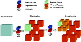
Graphical representation of the 3‐D wavelet transform.

It is well known in neuroimaging that when trying to estimate a signal of a known width, the width of the filter to be used should match that of the signal [Worsley et al., 1996]. However, in practice the signal in neuroimaging is usually of an unknown size and may occur in different places with different sizes, making it difficult to choose any one specific filter. This problem has been known for some time and methods have been proposed to overcome it [Worsley et al., 1996]. Wavelets offer an alternative “data driven” filter size. Each resolution, or level of decomposition, corresponds to a different filter size. Each wavelet coefficient can then be tested as to whether that coefficient is signal or noise, and appropriate steps based on this test can then be taken (see below). This can be viewed as a spatially adaptive model where the data helps determine which filter should be associated with each area.

There are other advantages of transforming the data using the wavelet transform. The properties of the wavelet transform allow more informed modeling of the data as signal tends to be represented by a small number of coefficients, whereas the noise tends to be spread evenly throughout the wavelet coefficients. This is even true when the noise is correlated in the image domain. As can be seen in Figure 2, the wavelet transform can decorrelate the data. Here simulated noise was generated with a 6‐mm Gaussian full‐width at half‐maximum (FWHM). This is often assumed to be the underlying spatial correlation structure in an fMRI dataset. As can be seen, the image space correlation function is a 6‐mm Gaussian kernel. However, when the data are transformed into wavelet space, the correlation between wavelet coefficients is significantly reduced, and thus many statistical procedures that would be difficult to perform on correlated data can now be performed on these essentially uncorrelated wavelet coefficients.

Figure 2.

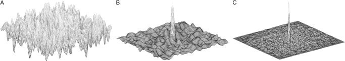
Simulated Gaussian 6‐mm noise image and the corresponding estimated spatial correlations in image space and wavelet space. As can be seen, the wavelet space has greatly reduced correlation.

The two properties above lead to the most significant part of the wavelet analysis. Having performed a wavelet transform of the data, direct application of the inverse wavelet transform returns the original data. Indeed, even if linear temporal modeling is performed (such as the general linear models popular in Statistical Parametric Mapping (SPM) [Ashburner et al., 1999]and other packages), and the subsequent parameter estimates transformed with the inverse wavelet transform, the resulting image space estimates will be identical to those estimates obtained using the same general linear model in image space, as if the wavelet transform was never performed. However, the decorrelation and sparse representation properties of the wavelet transform allow a thresholding step to be undertaken before the return inverse transformation of the parameters.

Thresholding the wavelet coefficients allows the estimates back in image space to have different properties compared with those of the underlying linear model. The temporal linear models of the type used in SPM are concerned with unbiased estimation. This, in effect, means that on average the estimated parameter will be the true value (given that the assumptions of the model are true). Indeed, the estimates obtained from these linear models are the “best linear unbiased estimates,” meaning that the variance of these estimates is minimal for all linear estimators that give unbiased estimates. However, there are different metrics for measuring whether an estimate is good or not. An alternative metric is that of Mean Squared Error (MSE) [Rice, 1995]. Here, both the bias of the estimate and the variance of the estimate are taken into account and their combined total (bias² + variance) is compared. An estimator is said to be better if the MSE is less than another estimator. This can be simply thought of in terms of a target (Figure 3).

Figure 3.

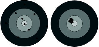
Diagrammatic representation of estimators with different mean squared error properties.

In the first target (left target), the overall average is unbiased (i.e., is in the centre) but the individual estimates can be a long way from the centre itself, whilst in the second target (right target), the average of the estimates is no longer the centre of the target (i.e., the estimates are biased) but each of the individual estimates is close to the centre of the target. Using an MSE metric, the second estimator would be characterized as better than the first estimator even though the second is a little biased. Indeed, SPM first smoothes the data to try to gain better MSE estimates and then uses linear models to fit the data; however, wavelet analysis provides adaptive smoothing compared with the fixed kernel smoothing of SPM. A large reduction in variance can be achieved using a large width filter, but this will lead to large bias.

Wavelet thresholding works on the principle of trying to find estimates that improve the MSE of the parameters. Different thresholding schemes can be used, such as nonlinear thresholding, where a wavelet coefficient is kept or removed depending on whether it is deemed to contain signal, or linear shrinkage, where the wavelet coefficients are shrunk towards zero depending on the level of noise they contain. Depending on the data and the underlying signal under investigation, different thresholders will have better or worse MSE properties. In the analysis of the FIAC data, linear shrinkage was used, as it has been shown to have better MSE properties for neuroimaging data than either unbiased estimators or those of nonlinear thresholders [Turkheimer et al., 2003].

Until recently, it had not been possible to obtain estimates of the variance or statistics of the parameters after the wavelet analysis. However, this problem has now been alleviated in different ways [Aston et al., 2005; Van De Ville et al., 2004], and there are now quantifiable error components associated with these estimates.

The above ideas lead to the following implementation (available in the Phiwave toolbox for SPM). Figure 4 gives the schematic for the analysis. The input data for the analysis is the result of standard spatial preprocessing, but omitting the final stage of spatial smoothing that is common in voxel‐based analyses. First, the wavelet transform of the original preprocessed data is taken. We refer to the wavelet transformed data as being in wavelet space. The resulting wavelet coefficients are then temporally modeled using standard methods, and the associated parameter estimates, their error variances, and residuals are calculated. Using these estimates and error variances in wavelet space, thresholding of the parameters is carried out, as is thresholding of the residuals. The parameters and residuals are then transformed back to the image domain using the inverse wavelet transform to recover parametric images and variance maps in the original image space [Aston et al., 2005].

Figure 4.

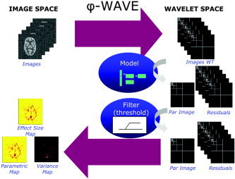
Schematic of the underlying methodology for the PhiWave analysis.

We implement random effects (cross‐subject) analyses using the same approach as standard voxel‐based packages: the input images are contrast images from a preliminary single subject analysis for each subject. The images can be the wavelet space unthresholded contrast images from a first level wavelet analysis, as above. Note that we obtain an identical set of images from taking the wavelet transform of the contrast images from a voxel‐based analysis that has used unsmoothed data.

Here we describe our own implementation of spatial wavelet analysis, instantiated in the Phiwave toolbox. We should also note that there is an excellent alternative method for doing spatial wavelet analysis—WSPM—that is also available as an SPM toolbox. WSPM is based on the methods determined in the article by Van De Ville et al. [2004]. While the principles are a little different from those in this article and the schematic of the Van De Ville et al. approach would vary slightly from ours (including methods to generate p‐values back in the image domain), the overall methodology is again aiming to take advantage of the signal representation properties of the wavelet transform.

Methodology for FIAC Data

In order to compare the results of the Phiwave wavelet analysis with a voxel‐based method, we analysed the FIAC data using a standard Phiwave procedure and a standard SPM2 procedure. The experimental paradigm can be found in the first article in this issue [Dehaene‐Lambertz et al., 2006]. The spatial preprocessing is identical for the two analyses, and was also based on SPM2, as the Phiwave toolbox imports the results of SPM preprocessing. Thus, the preprocessing procedure documented here is not specific to the Phiwave analysis, and is applicable to any dataset with the components contained in the FIAC dataset.

For simplicity, we only present results for the block version of the experiment. The event‐related version can also be analysed in a similar fashion.

Preprocessing.

We have described the preprocessing for these data at http://Phiwave.sourceforge.net/fiac/; this page includes batch scripts to reproduce the analysis. In what follows we refer to subjects using the subject numbers given by their directory in the data provided. For example, the first subject will be fiac0.

First, we excluded session 3 for subject fiac10, as the notes for the dataset commented that the subject was asleep during this session.

All the time series were reviewed with the tsdiffana utility http://www.mrc-cbu.cam.ac.uk/Imaging/Common/ downloads/SPMUtils/tsdiffana.tar.gz. This found a large number of high variance spikes within subject fiac8 and this subject was excluded from subsequent analysis. The datasets were then corrected for slice timing effects, and corrected for EPI distortion using the Fieldmap toolbox http://www.fil.ion.ucl.ac.uk/spm/toolbox/fieldmap/. As subjects fiac0, fiac5, and fiac11 did not have fieldmaps, these were also eliminated from subsequent analysis. The remaining datasets were then realigned and unwarped with the Unwarp toolbox http://www.fil.ion.ucl.ac.uk/spm/toolbox/unwarp/. We segmented the anatomical image for each subject into grey matter, white matter, and cerebrospinal fluid (CSF), and normalized the resulting definition of grey matter to the grey matter MNI template. We then resliced the EPI images to match the template using the normalization parameters.

Statistical analysis in SPM2.

For the SPM http://www.fil.ion.ucl.ac.uk/spm/ analysis, additional 5‐mm Gaussian spatial smoothing was performed on the data for single subject analysis, and 10‐mm Gaussian smoothing for the random effects analysis. We set up a model by defining the five conditions given in the documentation for the data:

• Same Sentence‐Same Speaker (SSt_SSp): a given sentence said by the same speaker was repeated six times;

• Same Sentence‐Different Speakers (SSt_DSp): a given sentence was repeated by six different speakers (three males, three females);

• Different Sentences‐Same Speaker (DSt_SSp): a given speaker produced six different sentences;

• Different Sentences‐Different Speakers (DSt_DSp): six different speakers (three males, three females) produced six different sentences.

• First Sentence in each block (FSt).

We modeled the events from each condition using the standard SPM HRF (Haemodynamic Response Function) method, which generates one regressor for each event, where each regressor consists of delta functions at the time of each event onset convolved with the standard HRF. To this model we added six columns of movement parameters (translations and rotations relative to the first scan in the session), giving 11 columns of regressors per session. We used a 120‐s high pass temporal filter, and ordinary least squares estimation was used in the data fitting.

If we then use the condition labels to refer to the parameter estimates for the regressor for that condition, we can express the main effect of Sentence in the usual way with this contrast: (DSt_DSp + DSt_SSp) – (SSt_DSp + SSt_SSp). The main effect of Speaker is given by (DSt_DSp + SSt_DSp) – (DSt_SSp + SSt_SSp), and the interaction can be expressed by (DSt_DSp – DSt_SSp) – (SSt_DSp – SSt_SSp). One possible interpretation of a positive value for such an interaction could be that there is a greater (more positive) difference between same and different sentences when the speaker also changes than when the speaker stays the same. The contrasts here could be expressed differently or expanded to include those with repetition priming from the first sentence, but as the main interest is that of differential response to speaker and sentences, these will not be reported.

We initially applied the default SPM intensity threshold masking for the SPM analysis. This has the effect of cutting off the activation signal near the edges of the brain. Therefore, it was deemed better not to apply the masking, even though this was a slight departure from the default standard analysis. Thus, the data were reanalysed using only a mask of voxels within the template brain and without threshold intensity masking and these are the SPM analyses presented here.

Phiwave analysis.

The Phiwave analysis consists of selecting a saved SPM model and estimating this in wavelet space. Thus, the temporal model for the Phiwave analysis was identical to the SPM2 model used. Phiwave automatically transforms the unsmoothed image data into wavelet space, before estimating the temporal model. Battle‐Lemarie wavelets, a class of wavelet functions that have been shown to be good for neuroimaging signals [Turkheimer et al., 2000a, b], were used in the transform. Four levels of decomposition were used; the elements in the lowest—and smoothest—level (known as approximation coefficients) were not subject to thresholding, as all these were regarded as signal. After the estimation of the temporal model, all of the other wavelet coefficients (detail coefficients) were subjected to Stein linear shrinkage as shown in Turkheimer et al. [2003]. The procedure for estimating variance maps in Aston et al. [2005]was also applied. These steps are summarized in the schematic of Figure 4.

Website

The associated Phiwave software for use with SPM (as an SPM toolbox) can be found at http://phiwave.sourceforge.net

RESULTS

It should be first noted that most of the results were consistent between the two methods of analysis. This is not particularly surprising, as they are both using parameters determined from the same temporal linear model, and while the spatial smoothing differs, both have previously been shown to model the data well. To illustrate the results of Phiwave analysis compared to SPM, we used the FSt (first sentence) contrast, as we were expecting strong bilateral activation in the auditory cortex at the single subject and random effects levels. We next show the results of the main effects and interaction of the Sentence and Speaker factors. All results are shown in neurological convention.

Figure 5 shows the contrast estimates for both the SPM and the Phiwave analysis for the contrast of first sentence against rest for a single subject, while Figure 6 gives the same images for a random effects analysis. We simply used the first retained subject in the analysis (fiac1) as the example single subject. As can be seen, and as expected, there are large effects bilaterally in the auditory cortices, in both single subjects and also in the overall combined random effect analysis. It can also be seen that there are only small differences in the effects map (top images) between the two analysis methods in this case. The main advantage of using the wavelet shrinkage methods is to improve mean squared error. As can be seen in Figures 5 (middle) and 6 (middle), this is achieved by a large reduction in the variance from the standard analysis to the wavelet analysis. This reduction (in terms of standard deviation) was about 40% for the single subject analysis and 25% for the random effects analysis, on average across the brain. These reductions in variance were consistent or greater across all contrasts, not just the first sentence vs. rest contrast.

Figure 5.

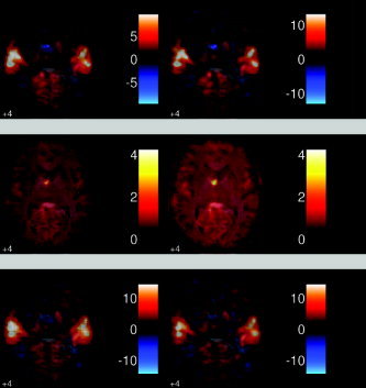
Single subject images for (left) PhiWave and (right) SPM2. This is the contrast of first sentence vs. rest. Effect (top), std of effect (middle), (pseudo)‐t statistic (bottom). As can be seen, there is clear activation in the auditory cortex, as expected. There is also a large reduction of the variance when using the wavelet transform compared with the standard SPM2 analysis.

Figure 6.

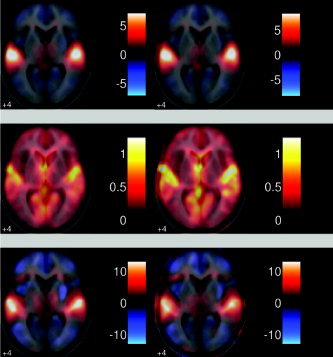
Random effect images for (left) PhiWave and (right) SPM2. This is the contrast of first sentence vs. rest. Effect (top), std of effect (middle), (pseudo)‐t statistic (bottom). As can be seen, there is clear activation in the auditory cortex; this is also seen in the single subject analysis. There is a large reduction of the variance when using the wavelet transform compared with the standard SPM2 analysis.

The pseudo t‐statistics for the single subject analysis can also be calculated (Fig. 5, bottom) and as can be seen, the wavelet statistics are similar to the t‐statistics from the standard analysis. There is slightly more structure present in the map from the wavelet analysis, as the smoothing has been adapted to the data, rather than using a predefined filter.

In Figure 7 the main effects of speaker and sentence type are compared. It can be seen that while there is little main effect of speaker, there is a pronounced left‐sided effect in response to same sentences vs. different sentences. These findings were also observed in the standard analysis, although the pattern was less smooth. Given the nature of the random effects analysis, smoother results might be deemed more appropriate, as there is generally considerable anatomical variance across subjects after standard spatial normalization.

Figure 7.

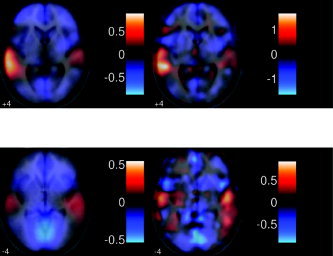
Random effect images (effect size) for (left) PhiWave and (right) SPM2 for the main effects of interest (top) DSt‐SSt and (bottom) DSp‐SSp. As can be seen, there is little effect of different speakers, but there is a large left‐sided effect for different sentences vs. same sentence. These findings were consistent between both methods of analysis.

For some contrasts, the results were not completely consistent between the two types of analysis. This can be most clearly seen in the random effects analysis of the interaction between the main effects of speaker and sentence type, which is shown in Figure 8. Both analyses pick out local effects of interaction, but in the Phiwave analysis, there are, in addition, more disperse, smoother effects that are not clearly seen in the SPM analysis. The Phiwave analysis identifies an interesting network of areas in the ventral visual stream and supplementary motor area, as well as ventral and medial prefrontal cortex.

Figure 8.

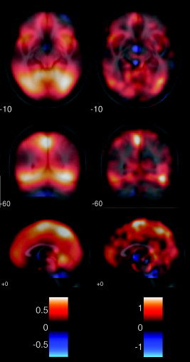
Random effects images (effect size) for (left) PhiWave and (right) SPM2 output for the effect of interaction. There is a large difference between the two methods of analysis. While both show localized effects, there are also large‐scale effects shown in the PhiWave analysis that are not obvious in the SPM2 analysis.

This would imply that different speakers did modulate the responses to the sentence type over rather large areas, rather than a few sharply defined locations. A fixed width 10‐mm smoothing kernel was used in the SPM analysis, while the wavelet analysis adapted the smoothing to the data and therefore was able to reconstruct both small‐ and large‐scale signals efficiently.

DISCUSSION

In this study a practical analysis of the FIAC data was performed using the wavelet techniques that make up the Phiwave analysis package. It has been shown that dramatic reductions in the variance of the contrasts can be achieved through the use of wavelet shrinkage. As the amount of shrinkage is determined from the data, the methodology can be seen to be data adaptive. This is different from standard techniques where the amount of filtering is predetermined before the size of the underlying signal is known.

The differences in the approach to filtering can lead to differences in the estimation of the effects, and this was most noticeable here in the FIAC data with regard to the random effect maps. The standard analysis found effects that were somewhat localized, whereas the Phiwave analysis estimated both localized and also smoother, more dispersed effects.

It should be remembered that when using analysis based on trying to minimize an MSE criterion, the subsequent estimates of the effects may be biased. This can be noticed in the differing ranges for the SPM and wavelet analysis. For wavelet analysis, the size of the effect is reduced, but this gains the advantage that the variance is also greatly reduced. As can be seen, the statistic images are in similar ranges, even though the effects are different sizes, due to the shrinkage steps used to reduce the variance.

Wavelet analysis in the spatial domain provides a powerful tool to search for signals of unknown sizes. The enhancement of analysis provided by these techniques will allow neuroscientists to understand the brain on many scales, as the data no longer needs to be considered using only one size of filter.

REFERENCES

- Ashburner J, Friston K, Holmes AP, Poline JB (1999): Statistical Parametric Mapping (SPM2 ed.). Website (http://www.fil.ion.ucl.ac.uk/spm): Wellcome Department of Cognitive Neurology .
- Aston JAD, Gunn RN, Hinz R, Turkheimer FE (2005): Wavelet variance components in image space for spatio‐temporal neuroimaging data. Neuroimage 25: 159–168. [DOI] [PubMed] [Google Scholar]
- Bullmore E, Fadili J, Breakspear M, Salvador R, Suckling J, Brammer M (2003): Wavelets and statistical analysis of functional magnetic resonance images of the human brain. Stat Methods Med Res 12: 375–399. [DOI] [PubMed] [Google Scholar]
- Cselenyi Z, Olsson H, Farde L, Gulyas B (2002): Wavelet‐aided parametric mapping of cerebral dopamine D2 receptors using the high affinity PET radioligand [11C]FLB 457. Neuroimage 17: 47–60. [DOI] [PubMed] [Google Scholar]
- Dehaene‐Lambertz G, Dehaene S, Anton JL, Campagne A, Ciuciu P, Dehaene GP, Denghien I, Jobert A, LeBihan D, Sigman M, Pallier C, Poline JB (2006): Functional segregation of cortical language areas by sentence repetition. Hum Brain Mapp 27: xx–xx. [DOI] [PMC free article] [PubMed] [Google Scholar]
- Mallat S (1999): A wavelet tour of signal processing. New York: Academic Press. [Google Scholar]
- Müller K, Lohmann G, Zysset S, von Cramon DY (2003): Wavelet statistics of functional MRI data and the general linear model. J Magn Resone Imaging 17: 20–30. [DOI] [PubMed] [Google Scholar]
- Percival DB, Walden AT (2000): Wavelet methods for time series analysis. Cambridge, UK: Cambridge University Press. [Google Scholar]
- Rice JA (1995): Mathematical statistics and data analysis, 2nd ed. Belmont, CA: Duxbury Press. [Google Scholar]
- Ruttimann UE, Unser M, Rawlings RR, Rio D, Ramsey NF, Mattay VS, Hommer DW, Frank JA, Weinberger DR (1998): Statistical analysis of functional MRI data in the wavelet domain. IEEE Trans Med Imaging 17: 142–54. [DOI] [PubMed] [Google Scholar]
- Taubman D, Marcellin M (2001): JPEG2000: image compression fundamentals, standards and practice. Heidleberg: Springer. [Google Scholar]
- Turkheimer FE, Brett M, Visvikis D, Cunningham VJ (1999): Multiresolution analysis of emission tomography images in the wavelet domain. J Cereb Blood Flow Metab 19: 1189–208. [DOI] [PubMed] [Google Scholar]
- Turkheimer FE, Banati RB, Visvikis D, Aston JAD, Gunn RN, Cunningham VJ (2000a): Modeling dynamic PET‐SPECT studies in the wavelet domain. J Cereb Blood Flow Metab 20: 879–93. [DOI] [PubMed] [Google Scholar]
- Turkheimer FE, Brett M, Aston JAD, Leff AP, Sargent PA, Wise RJ, Grasby PM, Cunningham VJ (2000b): Statistical modeling of positron emission tomography images in wavelet space. J Cereb Blood Flow Metab 20: 1610–8. [DOI] [PubMed] [Google Scholar]
- Turkheimer F, Aston JAD, Banati RB, Riddell C, Cunningham VJ (2003): A linear wavelet filter for parametric imaging with dynamic PET. IEEE Trans Med Imaging 22: 289–301. [DOI] [PubMed] [Google Scholar]
- Van De Ville D, Blu T, Unser M (2004): Integrated wavelet processing and spatial statistical testing of fMRI data. Neuroimage 23: 1472–1485. [DOI] [PubMed] [Google Scholar]
- Van De Ville D, Blu T, Unser M (2005): Isotropic polyharmonic b‐splines: scaling functions and wavelets. IEEE Trans Image Proc 14: 1798–1813. [DOI] [PubMed] [Google Scholar]
- Vidakovic B (1999): Statistical modeling by wavelets. New York: John Wiley & Sons. [Google Scholar]
- Worsley K, Marrett S, Neelin P, Evans A (1996): Searching scale space for activation in PET images. Hum Brain Mapp 4: 74–90. [DOI] [PubMed] [Google Scholar]