Exploring predictive and reproducible modeling with the single‐subject FIAC dataset

Abstract

Predictive modeling of functional magnetic resonance imaging (fMRI) has the potential to expand the amount of information extracted and to enhance our understanding of brain systems by predicting brain states, rather than emphasizing the standard spatial mapping. Based on the block datasets of Functional Imaging Analysis Contest (FIAC) Subject 3, we demonstrate the potential and pitfalls of predictive modeling in fMRI analysis by investigating the performance of five models (linear discriminant analysis, logistic regression, linear support vector machine, Gaussian naive Bayes, and a variant) as a function of preprocessing steps and feature selection methods. We found that: (1) independent of the model, temporal detrending and feature selection assisted in building a more accurate predictive model; (2) the linear support vector machine and logistic regression often performed better than either of the Gaussian naive Bayes models in terms of the optimal prediction accuracy; and (3) the optimal prediction accuracy obtained in a feature space using principal components was typically lower than that obtained in a voxel space, given the same model and same preprocessing. We show that due to the existence of artifacts from different sources, high prediction accuracy alone does not guarantee that a classifier is learning a pattern of brain activity that might be usefully visualized, although cross‐validation methods do provide fairly unbiased estimates of true prediction accuracy. The trade‐off between the prediction accuracy and the reproducibility of the spatial pattern should be carefully considered in predictive modeling of fMRI. We suggest that unless the experimental goal is brain‐state classification of new scans on well‐defined spatial features, prediction alone should not be used as an optimization procedure in fMRI data analysis. Hum Brain Mapp, 2006. © 2006 Wiley‐Liss, Inc.

INTRODUCTION

Data from functional magnetic resonance imaging (fMRI) are extremely rich in signal information but poorly characterized in terms of signal and noise structure [e.g., Lange et al.,1999; Skudlarski et al.,1999]. The dominant fMRI analysis methods so far focus on the detection of the spatial activation pattern and take advantage of only part of the signal information of the datasets. Motivated by the latest developments in machine learning, predictive modeling of fMRI data has the potential to expand the amount of information extracted and to enhance our understanding of brain systems by predicting brain states, rather than emphasizing the standard spatial mapping.

There are several other reasons to consider predictive modeling for fMRI data. First, from a Bayesian perspective there is no obvious advantage in estimating a spatial summary map from a priori knowledge of the experiment over trying to estimate these experimental parameters from the input patterns [Morch et al.,1997]. Second, prediction accuracy, which is potentially unbiased through cross‐validation, can be used along with other metrics (e.g., spatial pattern reproducibility) as a data‐dependent means of methodological validation [LaConte et al.,2003]. This validation reduces the likelihood of false insights due to limitations in acquisition or processing by uncoupling the testing of the “quality” of functional neuroimaging results from interpretations based on the neuroscientific knowledge base and associated neuroanatomic hypotheses [Strother et al.,2002,2004]. Third, predictive modeling explicitly uses the assumption that we have more reliable knowledge about the temporal aspects of the data than the spatial activation patterns. This is the same assumption implicitly used for generating Statistical Parametric Images (SPIs), interpreting “data‐driven” results, and modeling the hemodynamic response.

The number of investigations into predictive modeling of neuroimaging data has grown over the years [Haxby et al.,2001; Haynes and Rees,2005; LaConte et al.,2005; Mitchell et al.,2004; Morch et al.,1997; O'Toole et al.,2005]. This parallels the increased use of such machine learning techniques in science [Mjolsness and DeCoste,2001]. For example, the software package NPAIRS (Nonparametric Prediction, Activation, Influence, and Reproducibility reSampling), introduced by Strother, provides a formal predictive modeling framework for exploring multivariate signal and noise structures of neuroimaging data [LaConte et al.,2003; Shaw et al.,2003; Strother et al.,2002,2004]. The high‐dimension, low‐sample characteristics of fMRI data have also attracted the interest of more traditional machine learning groups.

In the context of predictive modeling, the goal of fMRI analysis is to learn a function that predicts a variable of interest (brain states or volume label, e.g., does a volume belong to a block where the subject was listening to the same sentence or to different sentences?) from features (e.g., voxels) of training samples. Given the high dimensionality of the feature space and the small sample size of fMRI datasets, “overfitting” (learning an overly complex classifier that has no predictive power on new samples) is a major issue. One way to avoid this is to use models with a relatively strong bias toward low complexity that are less susceptible to noise. This study considers five such models including linear discriminant analysis (LDA = Canonical Variates Analysis), Gaussian naive Bayes (GNB), GNB_pooled (a variant of GNB), logistic regression (LogReg), and linear support vector machines (SVM). The performance of these models in classifying and differentiating brain states was investigated on the basis of the Functional Imaging Analysis Contest (FIAC) data as a function of preprocessing steps and feature selection methods. A standard GLM analysis was also run as a baseline for comparison. The basic description of the fMRI experiment, subjects, and data acquisition methods related to the FIAC can be found in Dehaene‐Lambertz et al. [2006]. Our study uses only the block data provided for Subject 3.

MATERIALS AND METHODS

Preprocessing

Before feeding the functional data into a predictive model, we aligned each fMRI volume using the 3dVolReg program in AFNI (http://afni.nimh.nih.gov), spatially smoothed each axial slice in these volumes using a 2D Gaussian filter with an in‐plane full‐width half‐maximum (FWHM) of 6 mm, normalized the intensity by grand‐mean‐session scaling [Gavrilescu et al.,2002], and removed temporal trends and experimental block effects within a GLM framework as suggested by Holmes et al. [1997]. The temporal detrending was performed in NPAIRS by using a linear combination of four cosine basis functions with a cutoff value of 2 cycles.

In addition to the above‐noted preprocessing, we also removed several combinations of the following three types of volumes from the data before analysis: 1) volumes acquired during transitions between experimental states; 2) the two volumes following a positive transition to an active experimental state; 3) the remaining baseline volumes. Such volume removal simplifies class assignments, reduces effects of the hemodynamic response function (HRF), and also removes potentially nonstationary first sentence effects. Exceptions or deviations required for specific modeling techniques will be discussed in their respective sections.

A mask for the whole brain was generated using the 3dAutomask program in AFNI and applied prior to processing. In addition, a secondary mask omitting the lower 13 slices of the brain was also included to remove significant artifacts that we could not satisfactorily correct.

Classification Problem

In predictive modeling settings, the analysis of fMRI is essentially a classification problem. There are four conditions for the FIAC data (C1: same sentence, same speaker; C2: same sentence, different speaker; C3: different sentence, same speaker; C4: different sentence, different speaker) [Dehaene‐Lambertz et al., 2006]. Hence, it is natural to treat it as a 4‐class problem with the volumes in the same condition being assigned the same class label (1, 2, 3, or 4). Two 2‐class problems derived from the FIAC are: (1) differentiating between same sentence and different sentences (main sentence effect, reflecting the adaptation of the brain to the linguistic content that is independent of the speaker.); and (2) between same speaker and different speakers (main speaker effect, reflecting the adaptation of the brain to the speaker identity that was independent of the linguistic content). We focused on the main sentence effect in this study since our preliminary study revealed that the main sentence effect was much stronger than the main speaker effect and our primary goal was to compare predictive modeling approaches. In this case, all volumes in C1+C2 (same sentence) were assigned class –1 and those in C3+C4 (different sentences) class 1. For simplicity, we examined the binary classification problem (class = ±1) for all models, focusing on the main sentence effect. The 4‐class classification problem was only investigated using the LDA model.

Resampling Framework and Cross‐Validation

In our cross‐validation resampling framework, data were split into two partitions—a training set and a validation set with each run as the split unit. A cross‐validation procedure was then performed on this single split (only two runs in the FIAC data), generating two prediction accuracy estimates: training with run1 and estimating prediction on run2 and vice versa. The prediction accuracy was calculated as the proportion of the scans that were correctly classified in each validation run. The average of the two prediction accuracies was reported as the final result of the prediction metric (p). Besides the p, we also computed the Pearson's correlation coefficient between the SPIs generated over each split (run) as the spatial pattern reproducibility metric (r), and converted the SPI pair to a Z‐score volume as described by Strother et al. [1998,2002] and Tegeler et al. [1999]. Such reproducible Z‐score SPIs created from pairs of independent SPIs from the two runs will be referred to as rSPIs.

Predictive Models

For all predictive models we removed volume types 1–3 as described in the Preprocessing section.

Model of linear discriminant analysis

LDA looks for the linear transformation of a dataset that maximizes the ratio of between‐class variance to within‐class variance. This model assumes that all classes possess a multivariate Gaussian distribution with identical covariance matrices.

The LDA was performed on a principal component analysis (PCA) basis over each detrended, half‐split data in NPAIRS [Strother et al.,2002]. The number of principal components used controls the model complexity. For each preprocessing combination (smoothing and detrending), the LDA was performed on a variable number of principal components ([2,4,6,8,10,15,20,25,30,40] components were explored for 2‐class, and [5,10,15,20,25,30,35,40,50,60] components for 4‐class). The model (either 2‐class or 4‐class) for each preprocessing was tuned across different numbers of principal components (PC) by two different criteria: maximizing p alone or jointly maximizing r and p (minimizing the Euclidean distance between (1,1) and (r, p)) [LaConte et al.,2003; Shaw et al.,2003; Strother et al.,2004].

Models of GNB, GNB_pooled, LogReg, and SVM

Four more models, GNB, GNB_pooled, LogReg, and linear SVM, were investigated together with feature selection methods.

A voxel‐based simplification of LDA, GNB makes the same assumption as GLM that voxels are independent [Kjems et al., 2002]. It obtains one estimate of variance for each combination of voxel and class. A variant, GNB_pooled, uses data from all classes to estimate variance per voxel. GNB_pooled, therefore, produces a more biased estimate of the variance, but with lower variance of the variance estimate. Both GNBs are considered generative classifiers in that they model the conditional probability distribution of each class and use that with Bayes' rule to produce a predictor [Mitchell et al.,2004], which can be expressed as a linear function of the features. The GNB with pooled variance is a predictive analog of the standard GLM.

LogReg and linear SVM are the two discriminative linear classifiers we considered. Both classifiers directly learn a combination of features that can be used as a predictor. The 2‐class LogReg learns a linear combination of features to predict the ratio of the posterior class probabilities. The version of LogReg used in our study includes an additional regularization parameter—set to 1 in all experiments—that trades off the squared norm of the weight vector within the traditional conditional likelihood objective for LogReg [Hastie et al.,2001; Mitchell1997]. A linear SVM also learns a linear discriminant directly, but with the goal of finding the discriminant that maximizes the margin between examples of two classes. The margin is defined as the distance from the discriminant to the examples closest to it [Hastie et al.,2001; LaConte et al.,2005; Vapnik,1995]. Each of the above four models was applied to the preprocessed half‐split data in both the voxel and PC feature spaces. In the PC space, each model used as features the principal components obtained by applying singular value decomposition (SVD) to both runs simultaneously. This is different from the LDA model, where the PCs were obtained for each run separately to maintain strict training and validation‐set independence.

Feature Selection, Additional Preprocessing, and SPI Visualization

Feature selection is another way to deal with the problem of “overfitting” in fMRI classification. Feature selection is based on the informative extent of each feature measured by a “score” [Mitchell et al.,2004]. For a designated number N, a subset of the features with the top N scores will be selected. The three feature selection methods we used to compute the “score” were: intensity level (ILFS) [Mitchell et al.,2004], nested cross‐validation, and logistic regression [Hastie et al.,2001; Xing et al.,2001]. While the latter two are relatively common in high‐dimension machine learning, ILFS is more specific to fMRI. In ILFS, a one‐tailed t‐statistic was calculated for each voxel, checking the activation for each condition/class against the baseline. For any given condition/class, the voxels were ranked in descending order based on the t‐statistic (the voxel with the largest t‐statistic has rank 1). A final score was then generated as the lowest rank number across all conditions/classes for a given voxel. The feature selections were only performed on the models of GNB, GNB_pooled, LogReg, and linear SVM. Each feature selection method was used to select a varying number of features, based on which a classifier was trained. This selection and classification procedure was performed with 18 different sets of voxels (N from 25–2000) and 10 different sets of PCs (N from 5–200).

For the above four models, in addition to the general preprocessing steps in the Preprocessing section, two additional steps were performed: block averaging (AWB) and standard normalization (mean = 0 and StdDev = 1) of the volume intensity (STDNORM) across voxels. When using block averaging, the volumes in each block, or condition epoch, were averaged to one mean volume, producing four average scans per condition per run. STDNORM was performed on either each mean volume or on all volumes in each block. These two additional steps occurred either in the voxel space or the PC space. The combination of different options for each step in preprocessing (2(detrending: ON/OFF) × 2(AWB: ON/OFF) × 2(STDNORM: ON/OFF) × 2(space: voxel/PC)) resulted in 16 different datasets. Based on each preprocessed dataset, within the resampling framework each model was trained on the whole feature space or a fixed number of features selected by different feature selection methods. For each feature set, one prediction metric (p) was obtained using the cross‐validation procedure. The optimal p is reported across all combinations of feature selection methods and selected‐feature numbers together with the p for no feature selection.

In addition to the estimation of prediction accuracy, attempts were also made to generate spatial patterns for some models with high optimal prediction accuracy. All the classifiers described above use a weighted linear sum of features to reach a decision. The weight of the features can be visualized to see which features the classifier is using and how they influence the decision. This forms an SPI in which the voxel intensity reflects its discriminant weight. If a model is trained in voxel space, the discriminant it computes has as many weights as the number of features (voxels) selected for use. It is quite possible that the features selected during training with one half‐data split may not overlap much with those selected during training with the other half split. If a classifier is trained in PC space, the discriminant it computes again has as many weights as the number of features (components) selected for use (note, the components could either be selected by some feature selection methods or be designated as we did in LDA). However, as each component is a linear combination of voxels in the original space, it is possible to project the weights back so that an “equivalent” discriminant in voxel space is produced that covers the whole brain, reflecting the functional connectivity network. As an example, a detailed mathematical description of the SPI generation from LDA can be found in LaConte et al. [2003] and Strother et al. [2002].

GLM Analysis

A GLM analysis was performed on the block data using the 3dDeconvolve program in AFNI. The design matrix consisted of four columns corresponding to the covariates of interest, the four possible condition types. A voxel‐mean column was also included as a covariate of no interest. Detrending for the GLM analysis was accomplished by including four half‐cosine columns as covariates of no interest where appropriate. Individual SPIs were generated for different contrasts, in addition to an omnibus F‐statistic SPI for all conditions against the baseline. The GLM was implemented in two different ways to test removing volumes vs. using the HRF model. For GLM1 the design matrix was constructed based on a dataset with the type 1 and type 2 volumes described in the Preprocessing section removed. For GLM2 the HRF was modeled as the default Gamma function in AFNI. The four regressors in the design matrix were generated by convolving the reference function for each condition with the Gamma function. GLM2 appeared to produce somewhat stronger activation results and we used it to examine a range of contrasts for both individual and concatenated runs. The contrasts we tested were the main sentence effect (C4+C3‐C2‐C1), separate sentence effects for different (C4‐C2) and the same speakers (C3‐C1), and the largest effect indicated by our 4‐class CVA (C4‐C1). To facilitate comparison with multivariate models and to test run‐to‐run reproducibility, for analysis of individual runs an rSPI was created from a scatter plot of the two runs' SPIs.

Spatial Normalization

To obtain the Talairach coordinates of the activation locations in each region of the brain, we first normalized the structural image to the Talairach space in AFNI, and then coregistered the rSPIs to the Talairach‐normalized structural image with a 7 DOF affine transformation using FLIRT in FSL (http://www.fmrib.ox.ac.uk/fsl/).

If not annotated otherwise, all rSPIs are reported with an absolute Z threshold greater than 3.3 (corresponding to a two‐tailed, uncorrected P = 0.001).

RESULTS

A 4‐class LDA study performed on the whole brain revealed some significant artifacts. Figure 1 demonstrates the first dimension rSPI (Fig. 1a) and the corresponding canonical variate score (CVS) as a function of the class (condition) number (Fig. 1b). The CVS reflects significant condition effects. However, visually examining the rSPI, it seems very likely that these effects are driven by artifacts, possibly due to an interaction between susceptibility and condition‐related movement as opposed to “real” activation. We could not adequately correct for these artifacts. As an expedient feature selection approach to control artifacts, the lower 13 slices of the brain were omitted in the remainder of our predictive model analyses.

Figure 1.

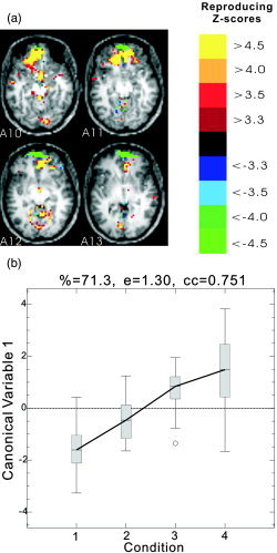
The first‐dimension results of 4‐class LDA analysis on the whole brain of Subject 3. a: Axial slices 10–13 of the Z‐score rSPI (see the Resampling Framework and Cross‐Validation section). b: Plot of canonical variates score (CVS) as a function of the condition. The data were preprocessed by 2D smoothing and detrending with a 1‐cycle cosine‐basis‐function cutoff. The LDA was performed on the first 10 principal components (PCs) of each run. In the CVS plot of each dimension, “%” is the percentage of total variance accounted for, “e” is the canonical eigenvalue, and “cc” is the canonical correlation coefficient (image right = brain left).

The results of prediction accuracy are summarized in Table I for the predictive models of GNB, GNB_pooled, LogReg, and SVM over Subject 3's dataset preprocessed with 16 different schemes. Unbolded and boldface rows contain results without and with block averaging (AWB), respectively. There are two accuracy results provided within each cell. The number within parentheses corresponds to no feature selection (namely, the prediction accuracy when using all available features); the number without parentheses is the optimal prediction accuracy across all combinations of feature selection techniques and selected feature numbers. By comparing results across different preprocessing choices and different models, we find that: (1) the number within parentheses is consistently lower across models and preprocessing schemes, suggesting feature selection assists in building a more accurate predictive model; (2) in either the voxel space or the PC space, detrending with the 2‐cycle cosine‐basis‐function cutoff consistently improves the optimal prediction accuracy value compared to no detrending, for the same preprocessing steps and model; (3) the SVM and LogReg often perform better than either of the GNB models in terms of the optimal prediction accuracy; and (4) the optimal prediction accuracy obtained in the PC space is typically lower than that obtained in the voxel space, given the same model and same preprocessing. However, these findings are only based on the results for a single subject. It would be necessary to analyze all subjects in order to determine whether the conclusions drawn generalize across subjects within this single study.

Table I.

Summary of the prediction accuracies for GNB, GNB_pooled, logistic regression, and linear SVM models

	GNB	GNB‐pooled	LogReg	SVM_linear
No detrending	0.66 (0.45)	0.71 (0.47)	0.74 (0.64)	/
	0.69 (0.50)	0.66 (0.47)	0.72 (0.59)	0.84 (0.56)
No detrending, STDNORM	0.70 (0.66)	0.72 (0.68)	0.72 (0.61)	/
	0.75 (0.72)	0.81 (0.69)	0.78 (0.66)	0.78 (0.62)
Detrended (cutoff: 2 cycles)	0.79 (0.74)	0.79 (0.76)	0.81 (0.76)	/
	0.91 (0.81)	0.94 (0.84)	0.94 (0.88)	0.94 (0.84)
Detrended (cutoff: 2 cycles), STDNORM	0.82 (0.74)	0.81 (0.75)	0.82 (0.78)	/
	0.91 (0.84)	0.91 (0.88)	0.94 (0.88)	0.94 (0.84)
No detrending, PC	0.53 (0.50)	0.61 (0.50)	0.69 (0.50)	0.71 (0.66)
	0.69 (0.50)	0.56 (0.50)	0.69 (0.62)	0.78 (0.50)
No detrending, PC, STDNORM	0.57 (0.47)	0.62 (0.53)	0.66 (0.66)	0.65 (0.65)
	0.62 (0.56)	0.56 (0.41)	0.75 (0.75)	0.75 (0.50)
Detrended (cutoff: 2 cycles), PC	0.64 (0.50)	0.72 (0.72)	0.78 (0.50)	0.82 (0.77)
	0.69 (0.50)	0.75 (0.47)	0.94 (0.81)	0.91 (0.50)
Detrended (cutoff: 2 cycles), PC, STDNORM	0.71 (0.53)	0.77 (0.62)	0.77 (0.77)	0.79 (0.79)
	0.56 (0.53)	0.66 (0.50)	0.78 (0.78)	0.94 (0.66)

Unbolded and boldface rows contain results without and with block averaging (AWB), respectively. The numbers within parentheses correspond to models trained using the entire feature space; the numbers not in parentheses indicate the optimal accuracy across all combinations of feature selection techniques and selected feature numbers.

Figure 2 illustrates the spatial patterns corresponding to the highest optimal prediction metric (0.94) in Table I, obtained by applying SVM to the detrended data with certain features selected in either the voxel space (Fig. 2a) or the PC space (Fig. 2b). In voxel space, 200 voxels were selected by ILFS for each run. The overlap between the two runs is only 10 of 200 voxels, indicating the instability of the feature‐selected spatial pattern. Figure 2a highlights the selected voxels in slices 14–18 when run1 was used as a training set. The overlap voxels are in yellow, while other selected voxels are in red. In PC space, 10 PCs were selected by nested cross‐validation for each run and then passed to the SVM model. The associated Z‐score rSPI had a reproducibility of 0.32 and is shown in Figure 2b.

Figure 2.

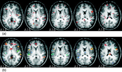
The spatial patterns corresponding to the SVM analysis of the detrended data with features selected in either voxel space (a) or PC space (b) (image right = brain left). In voxel space, 200 voxels were selected by the intensity level method (ILFS) for each run. Panel a highlights the selected voxels in slices 14–18 when run1 was used as a training set. The overlap voxels—those were also selected when run2 was used as a training set—are highlighted in yellow, others in red. In PC space, 10 PCs were selected by nested cross‐validation for each run and then passed to the SVM model. The resultant Z‐score rSPI is shown in panel b. See Figure 1a for the color scale of Figure 2b.

Table II lists the prediction metric (p) accompanied by the reproducibility (r) in parentheses for 2‐ and 4‐class LDAs. The LDA model was tuned either by maximizing the p only or by minimizing the distance from (r, p) to (1,1) (boldface row). For 2‐ and 4‐classes, p should be compared with their different performance levels for random guessing of 0.5 and 0.25, respectively. The reproducibility is dimension‐specific, and only the reproducibility for the first dimension is recorded.

Table II.

The prediction metric (p) accompanied by the reproducibility (r) in parentheses for 2‐ and 4‐class LDAs

	LDA (2 class)	LDA (4 class)
Detrended (cutoff: 2 cycles), PC	0.77 (r: 0.25)	0.39 (r: 0.24)
	0.69 (r: 0.52)	0.33 (r: 0.45)
No detrending, PC	0.66 (r: 0.16)	0.29 (r: 0.13)
	0.63 (r: 0.49)	0.21 (r: 0.16)

LDA model was tuned either by maximizing the p only or by minimizing the distance from (r, p) to (1,1) (boldface row). The reproducibility is dimension‐specific, and only the reproducibility for the first dimension is presented.

Figure 3 illustrates the results for the first three dimensions of the 4‐class LDA analysis on the masked brain (lower 13 slices were dropped). The masked brain was smoothed and detrended with a 2‐cycle cosine‐basis‐function cutoff. The number of the principal components passed to the LDA was 5. This PC number was determined by tuning the model using r and p simultaneously. Selected slices (14–18) of different dimensional rSPIs are shown in Figure 3a (row A: 1st dimension; row B: 2nd dimension; row C: 3rd dimension). Corresponding plots of the CVS as a function of the condition are shown in Figure 3b (from left to right). The first dimension CVS plot, which accounts for 74% of the total variance, illustrates a functional network (rSPI, row A, Fig. 3a) that reflects differences across all four conditions. The positive responses in Fig. 3a are weakest for same speaker same sentence (C1) and strongest for different speakers different sentences (C4). The high reproducibility of the dimension, 0.45, summarizes the strength of the spatial activation pattern associated with these differences. In the first dimensional rSPI, despite some artifacts in the ventricle, high intensity activation foci mainly occur in bilateral superior temporal lobes as well as in the inferior frontal gyrus (Table III). The second dimension accounts for 23% of the total variance, which, despite its low reproducibility of 0.07, illustrates a strong interaction centered in the right superior temporal gyrus. There is a large functional network modulation of the speaker effect for the same sentence with a smaller effect of opposite sign for different sentences. The third dimension looks like a simple speaker effect with very low reproducibility (0.02) and low total variance. The strongest activation in this dimension occurs in the left medial frontal gyrus. Table III reports the Talairach coordinates of the location with the peak Z‐score in each region of the brain for each dimension. These regions are delineated with the dotted black circles in Figure 3a. Targeted region of interest analysis and/or a group analysis in Talairach space is needed to further investigate these initial exploratory findings.

Figure 3.

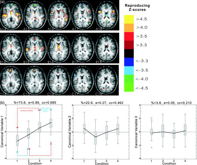
The first three dimensions of 4‐class LDA analysis on the masked brain (lower 13 slices removed to avoid artifacts). The masked brain was smoothed and detrended with a 2‐cycle cosine‐basis‐function cutoff. The number of the principal components passed to the LDA is 5. Selected slices (14–18) of different dimensional rSPIs are shown in panel a (row A: 1st dimension; row B: 2nd dimension; row C: 3rd dimension) (image right = brain left). The dotted black circles in panel a indicate the regions whose peak Z‐score locations are reported in Table III. Corresponding plots of canonical variates score (CVS) as a function of the condition are shown in panel b (from left to right). The “%,” “e,” and “cc” headings on the CVS plots are defined in the legend of Figure 1.

Table III.

Talairach coordinates of the peak Z‐score locations for 4‐class LDA results of Figure 3

Dimension and brain region	Talairach coordinates	Z‐score
1
Right superior temporal gyrus	52, −9, 7	5.63
Left superior temporal gyrus	−54, −38, 7	5.46
Left superior temporal gyrus	−57, −40, 7	4.77
Left medial frontal gyrus	−2, 66, 6	–6.44
Right insula	44, 15, 15	6.15
Left superior temporal gyrus	−48, −41, 16	5.20
Right inferior frontal gyrus	47, 18, 24	6.02
Left precentral gyrus	−47, 8, 25	6.12
2
Right superior temporal gyrus	59, −12, 11	4.94
3
Left medial frontal gyrus	−2, 63, 6	4.12

Figure 4a illustrates the rSPI for GLM2 using the Gamma HRF model. This omnibus F‐statistic–based rSPI is successful in detecting an overall effect of conditions against the baseline. These auditory and language effects are located primarily in the left and right perisylvian regions with a high reproducibility of 0.95 across runs. The correlation of the rSPI for GLM1 with the rSPI from GLM2 is 0.77, suggesting some dependence on removed volumes and the use of the HRF model. In general, the GLM2 results seem to have more activated voxels than for GLM1, so we focused on GLM2. The main sentence effect (C4+C3‐C2‐C1) for GLM2 with concatenated runs is illustrated in Figure 4b, row A. There is little perisylvian activity in slices A14–A16 to compare with the results in Figure 3a, and the few voxels that are weakly activated have uncorrected t values of only 2.5–3.5. Note that Figure 4 includes slices 12 and 13 that were masked out to avoid artifacts in the predictive modeling analyses (cf. Fig. 1a). The other SPIs for concatenated runs with different contrasts are similar, with little evidence of perisylvian activity. Analysis of individual runs was highly variable, with nonreproducible run‐to‐run SPI correlations of 0.08 for (C4+C3‐C2‐C1), 0.09 for (C4‐C2), 0.1 for (C3‐C1), and 0.03 for (C4‐C1). For comparison with the multivariate results in Figure 3 we displayed the SPI from run1 that had the strongest activations for (C4‐C1). There is evidence of perisylvian activity on the left side in slice A12, but only scattered voxels in A14–A16, and the pattern in run2 is quite different, leading to the low run‐to‐run SPI correlation of 0.03. Overall, the GLM seems unable to detect any reliable sentence, or other effect, between runs.

Figure 4.

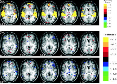
The spatial patterns for the GLM using the Gamma HRF model. a: Axial slices 12–16 of the Z‐score rSPI for the overall effect (four conditions vs. baseline). b: Axial slices 12–16 of the t‐statistic SPI for the main sentence effect with concatenated runs (row A) and the t‐statistic SPI for (Condition4–Condition1) with run1 (row B) (image right = brain left).

DISCUSSION

Advances in the interrelated fields of machine learning, data mining, and statistics have enhanced our capabilities to extract and characterize subtle features in datasets with high dimensionality but small sample size. Nevertheless, artifacts still make predictive modeling of fMRI a challenging task, particularly in individual subjects. Due to the existence of artifacts from different sources, high prediction accuracy alone does not guarantee that the classifier is learning a pattern of brain activity that may be usefully visualized, although cross‐validation methods do provide fairly unbiased estimates of true prediction accuracy. The reproducible spatial‐activation map provides a way to check which pattern of brain activity the model learns, and helps to prevent the model from learning obviously incorrect patterns. A typical example can be seen in the 4‐class LDA analysis of the FIAC data. When 4‐class LDA was performed on the whole brain, the tuned first dimension reproducibility was 0.41, while the prediction metric was 0.49. When 4‐class LDA was performed on the masked brain the overall prediction accuracy was reduced to 0.33. However, the rSPI in Figure 1a illustrates that the higher prediction accuracy from unmasked data was obtained, partly by learning movement‐ and susceptibility‐related artifact patterns. The sharp positive‐negative transition (yellow‐green) in the anterior of slices A10 and A11 is a characteristic eigenimage pattern of a moving boundary, and this occurs most strongly in this dataset, where there are susceptibility artifacts visible in the raw EPI images. To reduce the effect of artifacts on prediction, particularly LDA on a PCA basis, a very careful preprocessing is necessary to reduce structured and random noise variance because it is often much larger than the signal and/or is coupled to the stimulus. These results reinforce and extend the earlier results in Tegeler et al. [1999] comparing GLM and 2‐class LDA, which showed the sensitivity of an LDA to noise variance, particularly vascular artifacts at 4T.

The issue of how best to control excess noise variance through feature selection in multivariate predictive modeling of an fMRI time series is an open research question, although its importance may be somewhat model‐dependent. For example, LaConte et al. [2005] demonstrated that linear SVMs are less influenced by temporal detrending than are LDAs. One option is to select basis components (e.g., PCA component features) on which to build the predictive model. Strother et al. [2004] demonstrated artifact suppression with nonselective PCA tuning for an LDA of an fMRI group study. Formisano et al. [2002] demonstrated how ICA components might be selected to reduce artifacts prior to predictive modeling. Nevertheless we obtained mostly lower prediction results for PCA feature selection compared with spatial‐voxel feature selection in the present study (Table I). Another option is to use feature selection techniques targeted at specific artifacts, such as the mask used in this study. However, all such masks carry the risk of removing some true activation signal, as demonstrated in this study by the GLM results in masked slices A12 and A13 (Fig. 4a). Finally, the need to deal with subject‐dependent, structured artifacts is mitigated in group analyses, where they are likely to appear as somewhat random effects across subjects.

Feature selection definitely improves the predictive performance of the trained models in the experiments reported here, especially in the voxel space. However, given the total number of voxels to pick from, it is quite likely that the voxels selected during training with one run may not overlap much with those selected during training with another run. Our results show that in the voxel space, for an SVM with the optimal prediction accuracy as high as 0.94, the overlap of the 200 selected voxels between the two runs is only 10, indicating associated highly noisy and unreliable spatial patterns. One potential explanation is that more than 200 voxels contain correlated information useful for classification prediction, and therefore two or more different subsets of voxels may both lead to reliable predictions. An alternative explanation is that, given the very high dimension of the data, and the large number of feature subsets considered, it is possible with high probability to find voxel subsets that happen to perform well on cross‐validation tests without reflecting generally stable phenomena. This is related to the trade‐off between reproducibility and prediction that was emphasized by Strother and Hansen [Kjems et al.,2002; LaConte et al.,2003; Shaw et al.,2003; Strother et al.,2002,2004]. The reproducibility reflects the reliability of the SPI, while prediction reflects the generalizability of the model. A more obvious example can be seen in Table II, where the (r, p) values for 2‐ and 4‐class LDA with two different tuning methods are listed. It is very interesting to observe that r improves dramatically, while p only decreased slightly, when the tuning method was switched from maximizing p only to minimizing the distance of (r, p) from (1,1). Therefore, considering r and p simultaneously may be a better tuning choice in predictive modeling of fMRI. In essence, this tuning method gives an investigator a quantitative means of balancing confidence in matching known temporal information of the data with the priority of obtaining interpretable (and reproducible) summary images.

In our research, 2‐ and 4‐class LDAs were applied to the FIAC data analysis within a resampling framework. Both LDAs were able to easily detect the sentence effect that was not seen in the GLM analysis (Fig. 3a, row A vs. Fig. 4b, row A). Four‐class LDA further revealed strong, complex interaction effects with reproducible SPIs that appear to be contaminated with artifacts in the ventricles. A separate study would be needed to fully explore these interactions within and across subjects. Tuning by r and p enhances the robustness of the rSPIs across these LDA models. The first dimension rSPI of the 4‐class LDA (tuning by r and p) is correlated with the rSPI for the 2‐class LDA with correlation coefficients of 0.66 and 0.90 when the 2‐class LDA is tuned by p only, or by (r, p), respectively.

GLM is relatively insensitive to artifacts because it operates on a voxel‐by‐voxel basis. Although some artifactual voxels may be falsely identified as “active,” they do not corrupt the detection of other activated voxels. A similar insensitivity to artifacts will be shared by GNB results, but this seems to be reflected in reduced rather than improved prediction performance (Table I). On the other hand, LDA techniques using a PCA basis are built on the global variance structure in the data, and as a result significant artifacts can readily corrupt the identification of activated voxels and lead to artificially high (if coupled to the stimulus states) and low (if randomly occurring) prediction results. However, with appropriate preprocessing to control artifacts and the overall variance structure we have demonstrated that the LDA may detect activation effects (main sentence effect in 2‐ and 4‐class LDA) that the GLM cannot readily find (Fig. 4b). In addition, the 4‐class LDA provides a result that demonstrates interpretable, multiple complex interaction effects from a single analysis procedure. Nevertheless, such detection within a predictive modeling framework requires careful balancing of activation pattern visualization (i.e., reproducibility) with prediction performance. Unless the experimental goal is brain‐state classification of new scans, prediction alone should not be used as an optimization procedure in fMRI data analysis.

REFERENCES

- Dehaene‐Lambertz G, Dehaene S, Anton JL, Campagne A, Ciuciu P, Dehaene GP, Denghien I, Jobert A, LeBihan D, Sigman M, Pallier C, Poline JB (2006): Functional segregation of cortical language areas by sentence repetition. Hum Brain Mapp 27: xx–xx. [DOI] [PMC free article] [PubMed] [Google Scholar]
- Formisano E, Esposito F, Kriegeskorte N, Tedeschi G, Di Salle F, Goebel R (2002): Spatial independent component analysis of functional magnetic resonance imaging time‐series: characterization of the cortical components. Neurocomputing 49: 241–254. [Google Scholar]
- Gavrilescu M, Shaw ME, Stuart GW, Eckersley P, Svalbe ID, Egan GF (2002): Simulation of the effects of global normalization procedures in functional MRI. Neuroimage 17: 532–542. [PubMed] [Google Scholar]
- Hastie T, Tibshirani R, Friedman J (2001): The elements of statistical learning theory. New York: Springer. [Google Scholar]
- Haxby JV, Gobbini MI, Furey ML, Ishai A, Schouten JL, Pietrini P (2001): Distributed and overlapping representations of faces and objects in ventral temporal cortex. Science 293: 2425–2430. [DOI] [PubMed] [Google Scholar]
- Haynes JD, Rees G (2005): Predicting the stream of consciousness from activity in human visual cortex. Curr Biol 15: 1301–1307. [DOI] [PubMed] [Google Scholar]
- Holmes AP, Josephs O, Buchel C, Friston KJ (1997): Statistical modeling of low‐frequency confounds in fMRI. Neuroimage 5: S480. [Google Scholar]
- Kjems U, Hansen LK Anderson J, Frutiger S, Muley S, Sidtis J, Rottenberg D, Strother SC (2002): The quantitative evaluation of functional neuroimaging experiments: mutual information learning curves. Neuroimage 15: 772–786. [DOI] [PubMed] [Google Scholar]
- LaConte S, Anderson J, Muley S, Ashe J, Frutiger S, Rehm K, Hansen LK, Yacoub E, Hu XP, Rottenberg D, Strother SC (2003): The evaluation of preprocessing choices in single‐subject BOLD fMRI using NPAIRS performance metrics. Neuroimage 18: 10–27. [DOI] [PubMed] [Google Scholar]
- LaConte S, Strother SC, Cherkassky V, Anderson J, Hu XP (2005): Support vector machines for temporal classification of block design fMRI data. Neuroimage 26: 317–329. [DOI] [PubMed] [Google Scholar]
- Lange N, Strother SC, Anderson J, Nielsen F, Holmes AP, Kolenda T, Savoy R, Hansen LK (1999): Plurality and resemblance in fMRI data analysis. Neuroimage 10: 282–303. [DOI] [PubMed] [Google Scholar]
- Mitchell TM (1997): Machine learning. New York: McGraw‐Hill. [Google Scholar]
- Mitchell TM, Hutchinson R, Niculescu R, Pereira F, Wang XR, Just M, Newman S (2004): Learning to decode cognitive states from brain images. Machine Learn 57: 145–175. [Google Scholar]
- Mjolsness E, DeCoste D (2001): Machine learning for science: state of the art and future prospects. Science 293: 2051–2055. [DOI] [PubMed] [Google Scholar]
- Morch N, Hansen LK, Strother SC, Svarer C, Rottenberg DA, Lautrup B, Savoy R, Paulson OB (1997): Nonlinear versus linear models in functional neuroimaging: learning curves and generalization crossover In: Duncan J, Gindi G, editors. Information processing in medical imaging. New York: Springer; p 259–270. [Google Scholar]
- O'Toole AJ, Jiang F, Abdi H, Haxby JV (2005): Partially distributed representations of objects and faces in ventral temporal cortex. J Cogn Neurosci 17: 580–590. [DOI] [PubMed] [Google Scholar]
- Shaw ME, Strother SC, Gavrilescu M, Podzebenko K, Waites A, Watson J, Anderson J, Jackson G, Egan G (2003): Evaluating subject specific preprocessing choices in multisubject fMRI datasets using data‐driven performance metrics. Neuroimage 19: 988–1001. [DOI] [PubMed] [Google Scholar]
- Skudlarski P, Constable RT, Gore JC (1999): ROC analysis of statistical methods used in functional MRI: individual subjects. Neuroimage 9: 311–329. [DOI] [PubMed] [Google Scholar]
- Strother SC, Rehm K, Lange N, Anderson JR, Schaper KA, Hansen LK, Rottenberg DA (1998): Measuring activation pattern reproducibility using resampling techniques In: Carson RE, Daube‐Witherspoon ME, Herscovitch P, editors. Quantitative functional brain imaging with positron emission tomography. San Diego: Academic Press; p 241–245. [Google Scholar]
- Strother SC, Anderson J, Hansen LK, Kjems U, Kustra R, Sidtis J, Frutiger S, Muley S, LaConte S, Rottenberg D (2002): The quantitative evaluation of functional neuroimaging experiments: the NPAIRS data analysis framework. Neuroimage 15: 747–771. [DOI] [PubMed] [Google Scholar]
- Strother SC, LaConte S, Hansen LK, Anderson J, Zhang J, Pulapura S, Rottenberg D (2004): Optimizing the fMRI data‐processing pipeline using prediction and reproducibility performance metrics. I. A preliminary group analysis. Neuroimage 23: S196–S207. [DOI] [PubMed] [Google Scholar]
- Tegeler C, Strother SC, Anderson J, Kim SG (1999): Reproducibility of BOLD based functional MRI obtained at 4T. Hum Brain Mapp 7: 267–283. [DOI] [PMC free article] [PubMed] [Google Scholar]
- Vapnik V (1995): The nature of statistical learning theory. New York: Springer. [Google Scholar]
- Xing EP, Jordan MI, Karp RM (2001): Feature selection for high‐dimensional genomic microarray data In: Brodley C, Danyluk A, editors. Proceedings of the 18th International Conference on Machine Learning. San Francisco, CA: Morgan Kaufmann; p. 601–608. [Google Scholar]