Bayesian comparison of spatially regularised general linear models

INTRODUCTION

Functional Magnetic Resonance Imaging (fMRI) using Blood Oxygen Level Dependent (BOLD) contrast is an established method for making inferences about regionally specific activations in the human brain [Frackowiak et al., 2003]. From measurements of changes in blood oxygenation one uses various statistical models, such as the General Linear Model (GLM) [Friston et al., 1995b], to make inferences about task‐specific changes in underlying neuronal activity.

In this paper we propose analysing fMRI using a Bayesian Model Comparison (BMC) framework based on spatially regularised GLMs. Whilst model comparison can be thought of as a secondary concern, used primarily for fine‐tuning, an alternative perspective places it at the heart of the scientific endeavour. This is because in any mature scientific discipline there will be a candidate set of hypotheses. BMC can then be used to update ones beliefs about the competing hypotheses in light of experimental data. A more prosaic example is the analysis of data from factorial experimental designs using Analyses of Variance (ANOVA). This is a mainstay of scientific research [Winer et al., 1991]. To infer that manipulation of an experimental factor caused a significant effect one compares two models, one with that factor and one without.

In neuroimaging, BMC is used in the analysis of functional integration [Penny et al., 2004]. This allows inferences to be made about effective connectivity and how that connectivity changes as a function of perceptual or cognitive set. In analyses of functional specialisation, BMC has been used to select the optimal order of autoregressive noise models [Penny et al., 2003].

Model comparison can be implemented using classical or Bayesian inference. In classical inference, however, one is restricted to comparing nested models [Gelman et al., 1995]. Whilst this is sufficient for ANOVA, it is suboptimal in other domains. In this paper we show that a non‐nested approach is optimal for the comparison of hemodynamic basis sets.

In previous work we have developed a Bayesian framework that allows inferences to be made about regional activations using Posterior Probability Maps (PPMs) [Penny et al., 2005]. This has been extended by incorporating a spatial prior embodying our knowledge that evoked responses are spatially contiguous [Penny et al., 2005]. A key feature of that work is that it provides an approximation to the model evidence.

In thispaper we show how the model evidence can be used for model comparison and give details of the necessary computations. This provides a unified framework for Bayesian ANOVAs, Cluster of Interest (COI) analyses and the principled selection of signal and noise models. We also describe extensions to the framework that implement spatial and anatomical regularisation of noise process parameters.

The paper is structured as follows. In the next section we describe BMC and show how the model evidence can be appproximated. In later sections we describe our probabilistic model for fMRI and show how approximate inference can proceed. We also describe a variant of the model using ‘tissue‐type priors’ that make use of anatomical information. In the results section the method is applied to simulated data to illustrate the properties of COI analysis and to compare nested versus non‐nested model comparison of hemodynamic basis sets. Results on an event‐related fMRI data set illustrate Bayesian selection of signal and noise models and Bayesian ANOVA.

THEORY

Bayesian Model Comparison

Posterior model probabilities

Given a set of probabilistic models indexed by m = 1 … M and a data set Y, Bayesian Model Comparison (BMC) can be implemented as follows [Kass and Raftery, 1995]. Firstly, one requires a prior distribution over models, p(m). Typically this will be a uniform distribution indicating that no model is favoured a priori. One then needs the evidence for model m, p(Y|m). The evidence is not straightforward to compute but the next section shows how it can be approximated. From the model prior and model evidence one can then compute the posterior probability of model m using Bayes rule

(1)

This posterior distribution can be used in a number of ways. In Bayesian Model Averaging p(m|Y) provides a weighting for combining model predictions. This has been used, for example, to improve EEG source localisation [Trujillo‐Barreto et al., 2004].

In this paper we use p(m|Y) for BMC. In a later section, for example, we compare the evidence of models with different hemodynamic basis sets. All the examples in this paper assume a uniform prior over models ie. p(m) = 1/M. The model with the highest posterior probability will therefore also have the highest evidence. This means that the model evidence alone can also be used for model selection.

Approximating the model evidence

Given that model m has parameters θ, the evidence for model m can be written as

(2)

Taking logs, and writing the log‐evidence as L(m) ≡ log p(Y|m) gives

(3)

If we now take expectations with respect to, what for the moment we will regard as an arbitrary distribution, q(θ|Y,m) we get

(4)

This can be re‐arranged as follows

(5)

where the first term is known as the negative free energy [Neal and Hinton, 1998]

(6)

and the second term is the Kullback Leibler (KL) divergence [Cover and Thomas, 1991], which can be written generically for any probability densities q(x) and p(x) as

(7)

KL measures the discrepancy between two probability densities. It is equal to zero if the densities are identical and greater than zero otherwise. Because KL ≥ 0, Eq. (5) tells us that L(m) ≥ F(m). That is, the log model evidence is bounded below by F, and the closer q(θ|Y,m) is to p(θ|Y,m), the tighter the bound.

Equation (5) describes the fundamental relationship between model evidence, free energy and KL‐divergence. This relationship is used in the inference framework known as Variational Bayes (VB) [Beal, 2003]. In VB, the parameters of an approximate posterior density, q(θ|Y,m) (see later section) are updated to maximise F(m). This therefore maximises a lower bound on the model evidence. A number of methods now use this approach in the analysis of neuroimaging data [Penny et al., 2003, 2005; Sahani and Nagarajan, 2004; Sato et al., 2004; Wolrich et al., 2004].

Model comparison proceeds using F(m) as a surrogate for the model evidence, under the assumption that the bound in Eq. (5) is tight. This will be the case if the approximate posteriors are close to the true posteriors. In our previous work on modelling fMRI time series (see Section 5 in [Penny et al., 2003]) we have used Gibbs sampling to show that this is indeed the case.

It is also possible to approximate the model evidence using sampling methods [Beal, 2003; Gelman et al., 1995]. In the very general context of probabilistic graphical models, Beal and Ghahramani [2003] have shown that the VB approximation of model evidence is considerably more accurate than the Bayesian Information Criterion whilst incurring little extra computational cost. Moreover, model selection using VB is of comparable accuracy to a much more computationally demanding method based on Annealed Importance Sampling [Beal, 2003].

Computing the free energy

In this paper we will use F(m) as an approximation to the log evidence. This will form the basis of all model comparisons. This quantity can also be expressed in a more convenient form. If we expand the joint density p(Y,θ|m) = p(Y|θ,m)p(θ|m) and collect terms it can be written

(8)

where V(m) is the average log likelihood

(9)

and KL[q(θ|Y,m),p(θ|m)] is the divergence between the approximate posterior and the prior. The quantity F(m) therefore comprises two terms: (i) an accuracy term, the average log likelihood, and (ii) a complexity term, the KL divergence. This can be viewed as a complexity term because, as the number of parameters grows (ie. the dimension of θ) so does the KL.

Analysis of fMRI Time Series

To apply the model comparison framework we need a set of models m and for each model we must specify a set of parameters, θ, a prior distribution of those parameters, p(θ|m) and the likelihood p(Y|θ,m). Together, the likelihood and prior define a probabilistic generative model that we describe in the following section.

Generative model

We write an fMRI data set consisting of T time points at N voxels as the T × N matrix Y. In mass‐univariate models [Friston et al., 1995b], these data are explained in terms of a T × K design matrix X, containing the values of K regressors at T time points, and a K × N matrix of regression coefficients W, containing K regression coefficients at each of the N voxels. The model is written

(10)

where E is a T × N error matrix.

It is well known that fMRI data are contaminated with artifacts. These stem primarily from low‐frequency drifts due to hardware instabilities, aliased cardiac pulsation and respiratory sources, unmodelled neuronal activity and residual motion artifacts not accounted for by rigid body registration methods [Wolrich et al., 2001]. This results in the residuals of an fMRI analysis being temporally autocorrelated.

In previous work we have shown that, after removal of low‐frequency drifts using Discrete Cosine Transform (DCT) basis sets, low‐order voxel‐wise autoregressive (AR) models are sufficient for modelling this autocorrelation [Penny et al., 2003]. It is important to model these noise processes as parameter estimation becomes less biased [Gautama and Van Hulle, 2004] and more accurate [Penny et al., 2003]. Together, DCT and AR modelling can account for long‐memory noise processes. Alternative procedures for removing low‐frequency drifts include the use of running‐line smoothers or polynomial expansions [Marchini and Ripley, 2000].

In this paper, we adopt the approach taken in previous work. For a Pth‐order AR model, the likelihood of the data is given by (see equation 10 in [Penny et al., 2003])

(11)

where N() is the Normal density defined in Appendix E, at the nth voxel, a_n is a P × 1 vector of AR coefficients, w_n is a K × 1 vector of regression coefficients and λ_n is the observation noise precision. The vector x_t is the tth row of the design matrix and X_t is a P × K matrix containing the previous P rows of X prior to time point t. The scalar y_tn is the fMRI scan at the tth time point and nth voxel and d_tn = [y _{t − 1,n}, y _{t − 2,n}, …, y _{t − P,n}]^T. This shows that higher model likelihoods are obtained when the prediction error y_tn − x _t w _n is closer to what is expected from the AR estimate of prediction error. Because d_tn depends on data P time steps before, the likelihood is evaluated starting at time point P + 1, thus ignoring the GLM fit at the first P time points.

The voxel wise parameters w_n and a_n are contained in the matrices W and A and the voxel‐wise precisions λ_n are contained in λ. Appendices A, B and C describe the prior distributions over these parameters. Appendix B, for example, describes a prior over regression coefficients that enforces an automatic spatial regularisation using eg. Low Resolution Tomography (LORETA) or Gaussian Markov Random Field (GMRF) priors. These have been described in detail in previous work [Penny et al., 2005]. Together, the likelihood and priors define the generative model, which is portrayed graphically in Fig. 1. This generative model is identical to that described in our previous work [Penny et al., 2005], except that we have augmented the model so that the AR coefficients are regularised as described in the next section.

Figure 1.

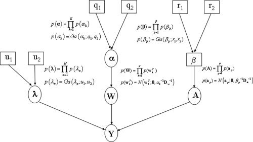
Generative model: The figure shows the probabilistic dependencies underlying our generative model for fMRI data. The quantities in square brackets are constants and those in circles are random variables. The spatial regularisation coefficients α constrain the regression coefficients W. The parameters λ and A define the autoregressive error processes that contribute to the measurements. The spatial regularisation coefficients β constrain the AR coefficients A. The graph shows that the joint probability of parameters and data can be written p(Y, W, A, λ, α, β) = p(Y|W, A, λ)p(W|α)p(A|β)p(λ|u ₁, u ₂)p(α|q ₁, q ₂)p(β|r ₁, r ₂), where the first term is the likelihood and the other terms are the priors. The likelihood is given in Eq. (11) and the priors are defined in greater detail in Appendices APPENDIX A: PRECISIONS, APPENDIX B: REGRESSION COEFFICIENTS, APPENDIX C: AR COEFFICIENTS.

AR priors

It is well established that the amount of temporal autocorrelation in fMRI data varies as a function of voxel position. This can be modelled using voxel‐wise AR processes [Bullmore et al., 1996; Penny et al., 2003; Woolrich et al., 2001; Worsley et al., 2002].

It has also been observed that the autocorrelation varies as a function of tissue type i.e. grey matter, white matter or Cerebro‐Spinal Fluid (CSF). For example, in AR(1) models, larger coefficients are observed in CSF [Penny et al., 2003].

It is an open question, however, as to whether tissue type is sufficient to explain the observed spatial variability. In this paper we address this question from a model comparison perspective by comparing two types of model. Each model regularises the estimation of voxel‐wise AR coefficients in a different way.

The first type of model uses a ‘tissue‐type prior’ that we define as follows. First, each voxel is labelled as belonging to one of S discrete categories. For example, s = {1,2,3} could correspond to the voxel belonging to (1) grey matter, (2) white matter or (3) CSF. This information can be derived from a segmentation of registered structural images [Ashburner and Friston 2003a]. Second, archetypal AR coefficient vectors are associated with each category. This is implemented by specifying a Gaussian distribution for each category. Appendix F describes these priors mathematically and shows how the means and precisions of the Gaussians can be estimated from the data.

The second type of model uses a spatial prior that takes into account voxel position. Following Woolrich et al. [2004] we use a GMRF prior. This has been shown to improve estimation of AR parameters, especially for the lower order coefficients. This prior is defined mathematically in Appendix C. It is also illustrated in the generative model in Figure 1. Similar spatial regularisation procedures, but based on Gaussian kernels, have been proposed in the context of classical inference [Gautama and Van Hulle, 2004; Worsley et al., 2002].

In later sections we show that our model comparison procedures are capable of detecting the correct type of variation (eg. spatial versus tissue‐type), and of indicating which is the better model for fMRI.

Approximate posteriors

This paper uses the VB framework [Beal, 2003] for estimation and inference. This requires the specification of an approximate posterior distribution whose parameters are updated so as to maximise the negative free energy, as described in an earlier section.

This paper uses the algorithm described in previous work [Penny et al., 2005] in which we assume that the approximate posterior factorises over voxels and subsets of parameters. This leads to a set of equations for updating the sufficient statistics of components of the approximate posterior shown in Figure 2. These update equations are also provided in the appendices. These appendices are self‐contained except for a number of quantities that are marked out using the ‘tilde’ notation. These are , , , and that are all defined in Appendix B of [Penny et al., 2003].

Figure 2.

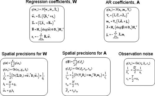
Approximate posteriors: The full approximate posterior distribution is q(W, A, λ, α, β) = [∏${}_{\mathit{\text{n}}\text{=1}}^{\mathit{\text{N}}}$ q(w_n)q(a_n)q(λ_n)] q(α)q(β). The boxes in the figure show each component of the approximate posterior along with update equations for their sufficient statistics.

Derivations of update equations that are new to this paper (see e.g. Appendixes C and F) have been omitted but follow the standard variational approach, which is also described in Appendix A of [Penny et al., 2005].

The central quantity of interest in fMRI analysis is our estimate of effect sizes, embodied in contrasts of regression coefficients. A key update equation in our VB scheme is, therefore, the approximate posterior for the regression coefficients. This is given by Eq. (B4) in the appendix. For the special case of temporally uncorrelated data we have

(12)

where B is a spatial precision matrix and r_n is the weighted sum of neighboring regression coefficient estimates.

This update therefore indicates that the regression coefficient estimate at a given voxel regresses towards those at nearby voxels. This is the desired effect of the spatial prior and it is preserved despite the factoristion over voxels in the approximate posterior. Equation (12) can be thought of as the combination of a temporal prediction X ^T y_n and a spatial prediction from r_n. Each prediction is weighted by its relative precision to produce the optimal estimate ŵ_n. In this sense, the VB update rules provide a spatio‐temporal deconvolution of fMRI data. Moreover, the parameters controlling the relative precisions, and , are estimated from the data. This means that our effect size estimates derive from an automatically regularised spatio‐temporal deconvolution.

Computing the free energy

The negative free energy, F(m), will be used to approximate the model evidence and can be computed using the expression in Eq. (8). It comprises two types of term: the average log likelihood and the KL terms. Appendix D shows how the average log likelihood is computed. For the KL terms we have (dropping the m's)

(13)

where W are regression coefficients, A are AR coefficients, λ are observation noise precisions and α and β are the spatial regularisation coefficients for W and A, respectively (Fig. 1). Appendix E shows in detail how each KL term is computed. It is also possible to re‐arrange the computation of F(m) to make it more efficient, as a number of terms in the average log‐likelihood cancel with those in the KL expressions (see e.g. Miskin and Mackay, 2000). We have not used this re‐arrangement, however, as it compromises the readability and extendability of the implementation.

When comparing models with the same type of spatial prior (ie. same D_w and D_a), and the same number of regression coefficients, K, and the same number of AR coefficients, P, there is no need to compute terms involving log |D_w| or log |D_a|. This saves time, especially for slices with large numbers of voxels. Otherwise, this log‐determinant must be computed.1 This can be implemented by eigendecomposition and then taking the sum of the log of eigenvalues greater than machine precision. This last step is necessary as the matrices are not full rank [Penny et al., 2005].

Because our approximation to the model evidence depends on the aforementioned KL terms, it will also depend on the constants that define the priors at the highest level of the model. These are the priors p(λ_n), p(α_k) and p(β_p), which have associated constants q ₁, q ₂, r ₁, r ₂, u ₁ and u ₂ (see Appendix A). In previous work, however, we have shown for example that the optimal AR model order is robust to variations in over several orders of magnitude (see Section 5.2 in [Penny et al., 2003]).

Unique contributions

It is possible to decompose the evidence for each model into a sum of unique contributions from each voxel

(14)

where

(15)

The computation of these voxel‐specific terms is described in detail in Appendices D and E.

Breaking the evidence down into contributions from each voxel has two advantages. First, the update equations need only be applied at voxels whose contribution, U_n(m), is still increasing. We envisage that this could speed the estimation process, although this has yet to be implemented. Second, the differences in voxel‐wise contributions between two models can be used to plot PPMs. For example, given two models with equal priors the posterior probability of model 2 at voxel n is given by

(16)

Because U_n(m) is a contribution to the log evidence rather than the log‐evidence per se, maps based on U_n(m) are ‘pseudo’‐PPMs rather than PPMs proper. Nevertheless, they should be useful in characterising regionally specific effects. This method is used in the context of Bayesian ANOVAs in a later section.

The pseudo‐PPMs we have defined are conceptually different from PPMs proper. They are not a numerical approximation to proper PPMs. This is because our models are spatially extended and the model evidence is only defined for a slice of spatially extended data. In the abscence of spatial correlation pseudo‐PPMs will correspond to proper PPMs.

Hemodynamic basis sets

It is well known that the shape of the hemodynamic response varies from voxel to voxel and from subject to subject [Zarahn et al., 1997]. This is accounted for in the context of GLM analyses by characterising the response using a hemodynamic basis set [Frackowiak et al., 2003]. For example, Friston et al. [1998] proposed the use of a ‘canonical’ basis function composed of a sum of gamma functions. This can be augmented to include two other basis functions, the derivative of the canonical with respect to time and the derivative with respect to dispersion. Together, these basis functions constitute an ‘Informed’ basis set [Henson, 2003]. For event‐related designs, other authors have proposed ‘selective averaging’ procedures. These are formally equivalent to the use of a Finite Impulse Response (FIR) basis set [Henson, 2003].

In this paper we consider use of the following hemodynamic basis sets. Unless otherwise specified the basis functions cover a 32 s period post‐stimulus. We use the seven standard options available in the Statistical Parametric Mapping (SPM) software [SPM, 2002] (i) Inf‐1: the canonical response, (ii) Inf‐2: the canonical plus temporal derivative, (iii) Inf‐3: the canonical plus temporal and dispersion derivatives, (iv) F: a Fourier basis set with 10 sinusoids covering 20s, (v) FH: as (iv) but with Hanning windows, (vi) Gamm3: a set of three Gamma basis functions and (vii) FIR: a finite impulse response with 10 2‐second windows.

FACE fMRI DATA

This paper uses an event‐related fMRI data set acquired by Henson et al. [2002]. This data and a full description of the experiments and pre‐processing are available from http://www.fil.ion.ucl.ac.uk/spm/data/. The data were acquired during an experiment concerned with the processing of images of faces [Henson et al., 2002]. This was an event‐related study in which greyscale images of faces were presented for 500 ms, replacing a baseline of an oval chequerboard that was present throughout the interstimulus interval (Fig. 3). Some faces were of famous people and were therefore familiar to the subject and others were not. Each face in the database was presented twice. This paradigm is a two‐by‐two factorial design where the factors are familiarity and repetition. The four experimental conditions are ‘U1’, ‘U2’, ‘F1’ and ‘F2’, which are the first or second (1/2) presentations of images of familiar ‘F’ or unfamiliar ‘U’ faces. The design is shown pictorially in Figure 3.

Figure 3.

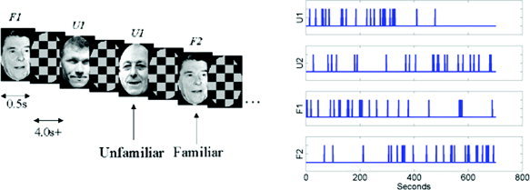
Face paradigm: (a) Experimental stimuli and (b) time series of stimuli presentation. [Colour figure can be viewed in the online issue, which is available at www.interscience.wiley.com.]

Images were acquired from a 2T VISION system (Siemens, Erlangen, Germany), which produced T2*‐weighted transverse Echo‐Planar Images (EPIs) with BOLD contrast. Whole brain EPIs consisting of 24 transverse slices were acquired every 2 s, resulting in a total of T = 351 scans. All functional images were realigned to the first functional image using a six‐parameter rigid‐body transformation. To correct for the fact that different slices were acquired at different times, time series were interpolated to the acquisition time of the reference slice. Images were then spatially normalized to a standard EPI template using a nonlinear warping method [Ashburner and Friston, 2003].

To implement a classical SPM analysis using Random Field Theory one usually spatially smooths the data at this stage [Brett et al., 2003]. But because our model incorporates a spatial prior that automatically determines the optimal amount of spatial regularization, this smoothing step is unnecessary.

We then computed the global mean value, g, over all time series, excluding non‐brain voxels, and scaled each time series by the factor 100/g. This makes the units of the regression coefficients ‘percentage of global mean value’. Each time series was then high‐pass filtered using a set of discrete cosine basis functions with a filter cut‐off of 128 s.

A structural scan was also acquired. This was normalised to the mean functional image and segmented into grey matter, white matter and CSF using the algorithm described in [Ashburner and Friston, 2003b]. Analysis of the functional data was restricted to within‐brain voxels, as identified by the structural segmentation.

RESULTS

Simulated Data

Comparing noise models

In this section we compare different assumptions about the prior distribution of AR coefficients using simulated data. The use of spatial GMRF priors assumes that AR coefficients vary smoothly across a slice, whereas the use of tissue‐type priors assumes that they vary about a small number of typical values. The simulations use first‐order AR models for simplicity. If the Signal to Noise Ratio (SNR) is sufficiently high, and our approximation, F, to the model evidence is sufficiently accurate then we should be able to use F to identify which prior was used to generate the data.

The leftmost column in Fig. 4 shows four different profiles of AR(1) coefficients. The first three profiles have one, two and three different typical values and the fourth has values that vary continuously as a function of position.

Figure 4.

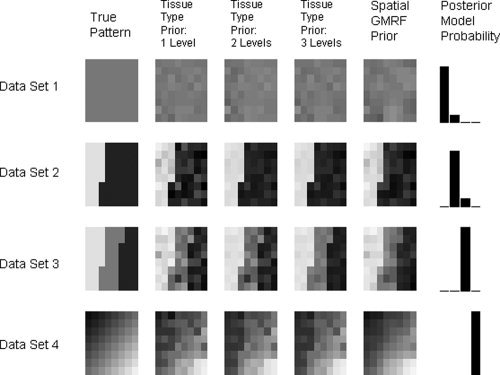
AR(1) images for synthetic data: Each row in this figure corresponds to analysis of a different data set. The leftmost column shows the AR(1) profile used to generate the data. The second, third and 4th columns show AR profiles as estimated by models with tissue‐type priors having 1, 2 and 3 (known) discrete levels, respectively. The fifth column shows the estimated profiles from models with spatial GMRF priors. The final column shows bar plots of the posterior model probabilities. The first three bars correspond to models with tissue‐type priors having 1, 2 and 3 levels and the fourth bar corresponds to the spatial GMRF model. These results show that our approximation to the model evidence can correctly detect the type of structure in the coefficients.

For each AR(1) profile we generated data as follows. We used a design matrix comprising two regressors, the first being a boxcar with a period of 20 scans and the second a constant. The design matrix, X, is therefore of dimension T × K (K = 2) and we chose T = 100 scans. We then used a K × N element regression coefficient matrix, W, whose elements were all set to 0.5. We chose N = 64 so that the coefficients could be reshaped into 8 × 8 images for display purposes. From this, we generated a simulated fMRI signal XW of dimension T × N. We also generated a simulated noise fMRI signal by first generating a Gaussian IID noise sequence with mean zero and precision λ = 1. For each voxel n, we then introduced a noise correlation as determined by the value of the AR coefficient at that voxel. The simulated data Y then comprised the simulated fMRI signal plus the simulated fMRI noise. Overall, we generated four data sets having the profile of AR(1) coefficients shown in Figure 4.

We then fitted each data set with four different models. The corresponding estimated profiles are shown in columns two to five in Figure 4. Columns two to four are estimates from tissue‐type priors with 1, 2 and 3 different categories, respectively. The fifth column contains estimates from a model with spatial GMRF priors. The final column shows the posterior model probabilities, p(m|Y). These posterior probabilities are computed using the constraint Σ_i p(m_i|Y) = 1, where i indexes the model and p(m_i|Y) ∝ p(Y|m_i) ∝ F(m_i) (under flat model priors p(m_i)). These show that the appproximation to the model evidence (see earlier section) is sufficiently accurate for the method to correctly detect the type of spatial structure in the data.

The estimate of F(m_i) entailed assigning each voxel to the appropriate ‘tissue‐type’ for the first three models. This is a component that is eschewed by the AR model with spatial GMRF priors.

As noted in an earlier section, our approximation to the model evidence is dependent on the constants that define the priors at the highest level of the model. We investigated this dependence by repeating the model fitting using different values for the relevant constants. Varying the prior mean precision of AR coefficients between 1 and 100 did not have a major effect on the choice of optimal model order.

COI analysis

If one has a strong prior hypothesis about the potential location of an activation then a Region Of Interest (ROI) analysis can be made. A region comprising a number of voxels is first chosen. This is often identified using localizer contrasts or scans (see e.g. [Kanwisher et al., 1999]). A single time series is then extracted using Principal Component Analysis or Singular Value Decomposition [Buchel and Friston, 1997], the mean operator or multiplication with a user‐specified activation shape [Brett et al., 2002]. Analysis is then based on this single ‘summary’ time series.

This section describes an alternative approach that we call COI analysis. Again, a region comprising a number of voxels is first chosen but the analysis is based on all time series in that region. The approach may also be viewed as a Bayesian cluster‐level inference as it shares the fundamental property of classical cluster level inference that anatomical specificity is traded off for increased sensitivity [Friston et al., 1995a].

To illustrate the properties of a COI analysis, we use simulations based on the experimental design of the face fMRI data in which models with different design matrices are compared. Design matrix 1, a ‘null’ model, comprises a column of 1s to model the mean response at a voxel. Design matrix 2 has a single additional experimental condition that was the presentation of a face regardless of factor or level. This was convolved with the canonical hemodynamic response function. Evidence in favour of a model using design matrix 2 allows one to infer that there was a response to faces.

Two types of data were generated, type 1 data sets using design matrix 1 and type 2 data sets using design matrix 2. Both types of data were generated for two‐dimensional clusters containing N = 1, 4, 9, 16 and 25 voxels. For each size of cluster we generated 500 data sets of each type. Overall, 2 × 5 × 500 = 5,000 data sets were generated. Both types of data were generated using regression coefficients fixed at unity across the patch. For data type 2 this represents a cluster of voxels that is uniformly active. The observation noise variance was set so that a range of sensitivities would be observed. This was achieved using a voxel‐wise SNR of 0.2 (we define SNR as the ratio of signal to noise standard deviation). This is very small for fMRI. The same observation noise variance was used for both types of data.

For each data set we then fitted four models: design matrices 1 and 2 with spatial GMRF priors and design matrices 1 and 2 with shrinkage priors. These shrinkage priors have been used in previous work [Friston et al., 2002] and do not make use of spatial information. A cluster was declared to be ‘active’ if the posterior probability of the model using design matrix 2 was greater than 0.999. We then computed the sensitivity and specificity of the inference over the 500 instances for each N. Overall, 4 × 5,000 = 20,000 models were fitted.

The specificity was found to be 100% for all sizes of cluster and for both types of prior. Figure 5 shows a plot of sensitivity as a function of number of voxels. This indicates that the effect is too weak to be detected at the single voxel level. But the signal is increasingly detectable as the cluster size increases. This shows the power of cluster‐level inference. Weak, diffuse signals can be detected at the ‘cluster‐level’ that cannot be detected at the ‘voxellevel’. The figure also shows that use of a spatial prior markedly increases this sensitivity. For the cluster containing 9 voxels the sensitivity is increased by over 30%.

Figure 5.

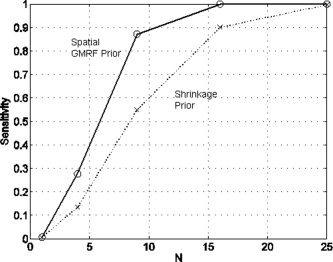
COI analysis for a uniformly activated region: The figure shows of a plot of sensitivity versus number of voxels in the cluster, N, for models using a spatial prior (circles and solid line) and a shrinkage prior (crosses and dotted line).

In a second set of simulations we repeated the above process but the regression coefficients were set to conform to a non‐uniformly activated cluster. A spatial Gaussian shape was chosen. The SNR was again chosen to obtain a range of sensitivities. This was achieved using SNR = 0.4. We again generated two types of data sets, with 500 instances of each type for each value of N.

Each data set was then fitted with six models: design matrices 1 and 2 with spatial GMRF priors, design matrices 1 and 2 applied to mean cluster activity, and design matrices 1 and 2 applied to the Principal Component (PC) of cluster activity. The first two models are used to assess the COI approach and the last four to assess two different ROI approaches. Clearly, the spatial parameters are redundant when modelling univariate summaries of regional responses like the mean or regional eigenvariate.

Clusters were again declared to be ‘active’ if the posterior probability of the model using design matrix 2 was greater than 0.999. Figure 6 shows a plot of sensitivity as a function of number of voxels, for each of the three approaches. Sensitivity reaches a peak for the cluster having 9 voxels. It then falls off due to the Gaussian nature of the spatial activation profile. This is seen most severely for the ROI approaches. Sensitivity is lowest using the mean time series and slighty higher using the PC time series. For the largest cluster, the COI approach is 20–30% more sensitive than the ROI approaches.

Figure 6.

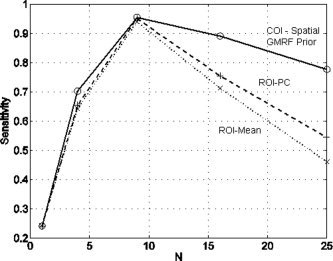
COI analysis for a non‐uniformly activated region: The figure shows of a plot of sensitivity versus number of voxels in the cluster, N, for a model using a spatial prior (circles and solid line), ROI analysis using the mean voxel time series (crosses and dotted line) and an ROI analysis using the principal component time series (plusses and dashed line).

These properties hold for all types of model comparison, whether it be an inference about a main effect, interaction (see later section) or selection of a hemodynamic basis set.

Comparing hemodynamic basis sets

This section describes the properties of nested versus non‐nested model comparison in the context of selecting an optimal hemodynamic basis set. As in the previous section, we use simulations based on the experimental design of the face fMRI data. Two types of data set are generated. The design matrix of type 1 data comprises the time series of delta functions, indicating the presentation of a face, regardless of factor or level, convolved with Inf‐3, the Informed basis set (see earlier section). Type 2 data sets use the same time series of delta functions but convolved with an FIR basis set having 10 time bins. Both types of data used design matrices also containing a constant term.

Type 2 data sets used FIR coefficients that were set to resemble the canonical response but with a pronounced undershoot. These non‐canonical undershoots have been observed by the authors in previous work, and so make an interesting hypothetical signal. Type 1 data sets were generated by projecting noise‐free type 2 data onto the Inf‐3 basis set. Type 2 data therefore contains a subtle effect that can be captured by an FIR basis but not by Inf‐3. Noise‐free versions of each type of data are shown in Figure 7. The difference between these noise‐free time series constitutes our signal of interest.

Figure 7.

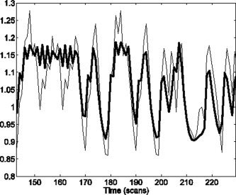
Noise‐free time series: From type 2 data (thin line), generated from an FIR model, and type 1 data (thick line), generated from a best fitting Informed basis set model. These data were used to compare the sensitivity of nested versus non‐nested model comparison, in the context of selecting an optimal hemodynamic basis set.

Noise was then added to each type of data set, as in the previous section, such that the noise level would provide a range of sensitivities. This was achieved using SNR = 0.6. Again, 500 data sets of each type were generated for each cluster size. Overall, 2 × 5 × 500 = 5,000 data sets were generated.

We then fitted three different models to each data set. Model 1 used an Inf3‐basis, model 2 an FIR basis and model 3 used an augmented design matrix containing both an Inf3 and FIR basis. Model 1 is therefore ‘nested’ within model 3. Comparing the evidence of model 2 to model 1 constitutes a non‐nested model comparison, whereas comparing the evidence of model 3 to model 1 constitutes a nested model comparison. The equivalent nested model comparison in classical inference is a standard approach for comparing basis sets in functional imaging using the ‘extra sum of squares’ principle [Henson et al., 2001].

Figure 8 plots the sensitivity of nested and non‐nested model comparison approaches. First, we note that the subtle undershoot effect cannot be detected at the voxel level. But as the clusters get larger the effect becomes increasingly detectable. Moreover, it is clear from the figure that non‐nested model comparison is more sensitive. For the cluster with 9 voxels, for example, the non‐nested approach is nearly twice as sensitive.

Figure 8.

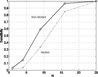
Nested versus non‐nested: The figure shows of a plot of sensitivity versus number of voxels in the cluster, N, for non‐nested model comparison (circles and solid line) versus nested model comparison (crosses and dotted line).

Face fMRI Data

Comparing noise models

This section compares spatial versus tissue‐type AR priors on the face fMRI data. We used a GLM with a design matrix where each level of each factor is represented separately. Each event type was convolved with the Inf‐2 basis set. An additional constant term gives 9 regressors.

We then compared a number of approaches for specifying the AR component of the model. Whilst the model evidence can be used to select the optimal model order, as shown in Penny et al. (2003), the focus of this section is on comparing spatial versus tissue‐type priors. We therefore used an AR model order of P = 1 for all comparisons.

We compared four different priors. The first three are tissue‐type priors which use (i) a single Gaussian for all voxels, (ii) three Gaussians, one for voxels in grey matter, one for white matter and one for CSF, (iii) two Gaussians, one for voxels in CSF (as defined using a spatially smoothed and thresholded CSF mask) and the other for the remaining voxels and (iv) a spatial GMRF prior. Prior (iii) was included in an attempt to improve the correspondence between the observed structure in the functional data (AR images) and the segmentation obtained from the structural data. Various spatial smoothing and thresholding operators were fine‐tuned so as to obtain the best results possible.

Figure 9 shows the estimated AR coefficients for priors (iii) and (iv) for selected slices. The corresponding images for priors (i) and (ii) are visually very similar to the prior (iii) images. Estimates using the GMRF prior are smoother, as one would expect. We now turn to a comparison of the model evidence.

Figure 9.

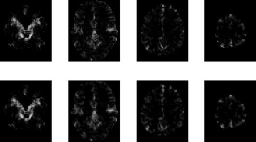
AR(1) images for face data: The top row shows estimated profiles from a tissue‐type prior (smoothed CSF versus other, prior (iii)) and the bottom row shows the estimated profiles from models with spatial GMRF priors. Columns in this figure show results for slices z = −27, 3, 33 and 63 mm.

Prior (i) had the lowest evidence in 95% slices. This indicates that there is tissue‐type structure in the pattern of AR coefficients (as priors (ii) and (iii) had higher evidence). Whilst this is evident from the images themselves and is widely recognised, our framework allows this inference to be made using a statistical test by evaluating the posterior beliefs that correspond to the differences in evidence. This posterior belief was unity for 95% slices.

Prior (ii) had the third highest evidence in 70% slices and prior (iii) had the second highest evidence in 70% of slices. This reflects our extensive efforts to improve the correspondence between the observed structure in the functional data (AR images) and the segmentation obtained from the structural data.

Despite these efforts, however, models with the spatial GMRF prior had the highest evidence in all slices examined. This shows that although tissue‐type effects are strong, they are not sufficient to explain the observed spatial variability in temporal autocorrelation.

Analysis of variance

We now present a Bayesian Analysis of Variance (ANOVA) for the face fMRI data. The presentation of faces conforms to a factorial design with two factors, familiarity and repetition. There are therefore four putative effects of interest: (i) the average effect of presenting faces, (ii) the main effect of repetition (iii) the main effect of familiarity and (iv) the interaction between repetition and familiarity.

As described in [Winer et al., 1991] (see also [Henson and Penny, 2003]), ANOVA is fundamentally a model comparison procedure. To test for our putative effects we therefore fitted a number of models to the data. For each model, all experimental conditions were modelled by convolving the appropriate stimulus functions with the Inf‐2 hemodynamic basis set. The design matrix of Model 1, a ‘null’ model, comprised a column of 1s to model the mean response at each voxel. Model 2 had a single additional experimental condition, which was the presentation of a face regardless of factor or level. Model 3 had two conditions, first or second repetition regardless of familiarity. Model 4 had two conditions, familiar or unfamiliar regardless of repetition. Model 5 had a design matrix containing all the conditions from models 3 and 4 (i.e. both main effects but no interaction). Model 6 had a ‘full’ design matrix comprising four conditions where each level of each factor is entered separately (i.e. all effects).

Voxel‐wise contributions to the approximate log‐evidence were computed for each model, U_n(m). These were then compared to assess putative experimental effects. For (i) the average effect of presenting faces we compared models 1 and 2, for (ii) the main effect of repetition we compared models 2 and 3, for (iii) the main effect of familiarity we compared models 2 and 4 and for (iv) the interaction between repetition and familiarity we compared models 5 and 6.

Figure 10 shows a map of the average effect of presenting faces for selected slices. Figure 11 shows a map of the main effect of repetition. In each figure the top row shows a map of the relevant difference in contribution to the approximate log‐evidence, U_n(m ₁) − U_n(m ₂), and the bottom row shows the same but thresholded so that the corresponding posterior probability, computed using Eq. (16), is greater than 0.999. For this subject there is a large bilateral occipital and fusiform response to the main effect of faces (Fig. 10) but no repetition effect (Fig. 11). The familiarity and interaction effects were also absent in this subject and so have not been presented.

Figure 10.

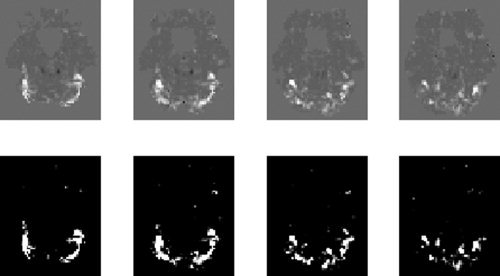
Average effect of faces: The top row shows maps of the difference in contributions to the log evidence, U_n(2)−U_n(1), for slices z = −24, −21, −18 and −15 mm. The bottom row shows the same map but thresholded so that only effects with a posterior probability greater than 0.999 (difference in log evidence = 4.6) survive.

Figure 11.

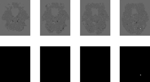
Main effect of repetition: The top row shows maps of the difference in contributions to the log evidence, U_n(3)−U_n(2), for slices z = −24, −21, −18 and −15 mm. The bottom row shows the same maps but thresholded so that only effects with a posterior probability greater than 0.999 (difference in log evidence = 4.6) survive.

Comparing hemodynamic basis sets

This section compares models with different hemodynamic basis sets. We use the seven options described in earlier section. The basis functions were convolved with stimulus functions corresponding to all four experimental conditions.

The approach is illustrated on COIs from three regions centred on left occipital cortex (LOC) x = −45, y = −60, z = −24 mm, right occipital cortex (ROC) x = 45, y = −66, z = −24 mm and sensorimotor cortex x = 36, y = −9, z = 66 mm. All COIs were 9 mm spheres and contained 83, 41 and 33 voxels, respectively. We also optimised the Hanning‐windowed Fourier and FIR basis sets by selecting the number of time‐bins and bin‐size that gave the highest model evidence.

Despite this the model evidence favours strongly an Informed basis set for all of the regions, as shown in Figure 12. The set Inf‐2 is preferred for LOC and Inf‐3 for the others. The differences in log evidence provide posterior probabilities of unity in favour of the most probable model. We also repeated the analyses with smaller COIs, but the results were much the same, with the informed basis sets always being preferred with high posterior probability (≥ 0.95).

Figure 12.

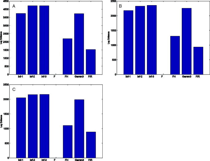
Comparing hemodynamic basis sets: The bar plots show the log‐evidence for each hemodynamic basis set for COIs in (a) LOC x = −45, y = −60, z = −24 mm, (b) ROC x = 45, y = −66, z = −24 mm and (c) Sensorimotor Cortex x = 36, y = −9, z = 66 mm. The evidence values have been normalised (by subtraction) so that the minimal log‐evidence is zero. [Colour figure can be viewed in the online issue, which is available at www. interscience.wiley.com.]

DISCUSSION

We have presented a unified framework for the analysis of fMRI data based on Bayesian comparison of spatially regularised GLMs. This allows for Bayesian ANOVAs, COI analysis and the principled selection of signal and noise models.

COI analysis is similar to an ROI approach but all time series in a region are used rather than a single ‘representative’ time series. Our simulations have shown that, for non‐uniformly activated regions the COI approach is substantially more sensitive. The COI approach may also be viewed as a Bayesian cluster‐level inference as it shares the fundamental property of classical cluster‐level inference that anatomical specificity is traded‐off for increased sensitivity. As is the case for classical inference, Bayesian cluster‐level inferences are more sensitive to weak, diffuse activations than are voxel‐level inferences. For diffusely activated regions this sensitivity increases with number of voxels in the region. Moreover, the use of spatial regularisation increases that sensitivity yet further. Unlike classical cluster‐level inferences [Friston et al., 1995a], a primary ‘height’ threshold is not required.

Bayesian ANOVAs can be implemented in two ways (i) using COI analysis or (ii) to produce pseudo PPMs for the whole image volume. The term ‘pseudo’ is used as these probabilities are based on contributions to the model evidence rather than the model evidence per se. These PPMs show voxels expressing overall effects, main effects or interactions.

In previous work we have shown how PPMs can be used to make inferences about regionally specific effects [Friston et al., 2002]. The approach is based on computing the probability that a contrast of parameter estimates is larger than a user‐specified effect size. For example, in primary sensory areas only effect sizes greater than 1% of global brain activity may be deemed biologically relevant. PPMs based on Bayesian ANOVAs, however, do not require the specification of an effect size threshold. This can be viewed as an advantage or a disadvantage depending on your perspective. On the one hand, imagers are unable to describe the effects that interest them so precisely, but on the other, they have one less parameter to specifiy.

A disadvantage of the Bayesian ANOVA approach, which we have described, is that a family of models must be fitted, which is obviously more computationally demanding than fitting a single model. This is not a problem for a COI analysis where models can be fitted in seconds, but it is potentially a problem for the production of PPMs. Fitting the six models required to produce a full ANOVA took 3 h of computer time.

An alternative to PPMs here is to make inferences based on F‐maps, as is standard in neuroimaging [Kiebel, 2003]. It is also possible to make ANOVA‐like Bayesian inferences about effect sizes based on multivariate Gaussian posteriors. The generic approach is described in Box and Tiao [1992].

We have also shown how our framework can be used for the principled selection of signal and noise models. We have illustrated its use on a single‐subject event‐related fMRI study of face processing. The following observations are therefore specific to our analysis of this data. Whether or not they apply generically to fMRI remains to be seen.

The framework was applied to determine the optimal regularisation method for an AR model of fMRI noise processes. Two types of regularisation were compared: (i) a spatial prior which assumes that AR coefficients vary smoothly across the brain and (ii) a ‘tissue‐type’ prior which assumes they vary about a small number of tissue‐specific values. BMC showed spatial priors to be better. Our results therefore show that tissue type is not sufficient to explain the observed spatial variability in temporal autocorrelation. The largest single source of this variability appears to be the strong autocorrelation observed close to the cerebral arteries, as shown for example in the plots on the left‐most side of Figure 9. Unless one has angiographic data, these regions are not easily delineated. The spatial prior approach can, however, automatically accomodate these variations.

The framework was also applied to determine the optimal basis set for describing the hemodynamic response. We have shown that the previously established method of nested‐model comparison [Henson et al., 2001] is sub‐optimal. Application of the optimal non‐nested framework revealed the ‘informed basis set’ to be the optimal choice in a number of COIs.

We now turn to a discussion of future work. Application of tissue‐type‐priors to regression coefficients is one simple extension. This would use zero mean Gaussians with prior variances that depend on tissue type. Low prior variances in CSF and white matter could be implemented using equivalents of the Gamma priors in Appendix F. Whether these models would be better than the spatial GMRF priors in this paper (based entirely on functional data) is an issue that can be resolved using the model comparison framework. In a similar vein, we are currently working on spatial‐basis set priors, that include e.g. wavelets, as an alternative to GMRFs.

APPENDIX A: PRECISIONS

Priors

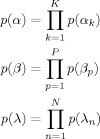
We use Gamma priors on the precisions α, β and λ

(A1)

(A2)

where () is defined in Appendix E. Gamma priors were chosen as they are conjugate priors for Gaussian error models. The parameters are set to q ₁ = r ₁ = u ₁ = 10 and q ₂ = r ₂ = u ₂ = 0.1. These parameters produce Gamma densities with a mean of 1 and a variance of 10. The robustness of model selection to the choice of these parameters is discussed in an earlier section.

Posteriors

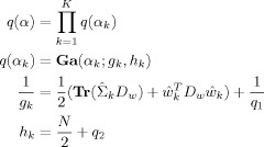
The approximate posteriors are also Gamma densities. For the precisions of the regression coefficients, we have

(A3)

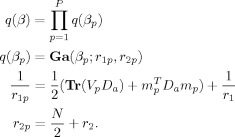
For the precisions of the AR coefficients, we have

(A4)

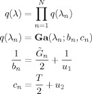
For the precisions on the observation noise, we have

(A5)

where is the expected prediction error defined in Appendix B of Penny et al. [2003].

APPENDIX B: REGRESSION COEFFICIENTS

Priors

For the regressions coefficients, we have

(B1)

where D_w is a spatial precision matrix. This can be set to correspond to e.g. a LORETA or GMRF prior, as described in earlier work [Penny et al., 2005]. These priors are specified separately for each slice of data. Specification of three‐dimensional spatial priors (i.e. over multiple slices) is desirable from a modelling perspective but is computationally too demanding for current computer technology.

We also write w_v = (W), w_r = (W^T), w_v = H_ww_r where H_w is a permutation matrix. This leads to

(B2)

where B is an augmented spatial precision matrix given by

(B3)

This form of the prior will be used in the derivation of KL‐divergences in Appendix E.

The aforementioned Gaussian priors underly GMRFs and LORETA and have been used previously in fMRI [Penny and Flandin, 2005] and EEG [Marqui et al., 1994]. They are by no means, however, the optimal choice for imaging data. In EEG, for example, much interest has focussed on the use of L^p‐norm priors [Auranen et al., in press] instead of the L ²‐norm implicit in the Gaussian assumption. Additionally, we are currently investigating the use of wavelet priors. This is an active area of research and will be the topic of future publications.

Posteriors

We have

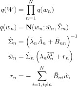(B4)

where is defined as in Eq. (B3) but uses instead of α. The quantities à _n and are expectations related to autoregressive processes and are defined in Appendix B of Penny et al. [2003]. In the absence of temporal autocorrelation we have à _n = X^T X and . The above density can be written as a distribution over w_v

(B5)

where and . This form of the posterior will be used in the derivation of KL‐divergences in Appendix E.

APPENDIX C: AR COEFFICIENTS

Priors

Similarly, for the AR coefficients, we have

(C1)

Again, D_a is a user‐defined spatial precision matrix, a_v = (A), a_r = (A^T) and a_v = H_aa_r where H_a is a permutation matrix. We can write

(C2)

where J is an augmented spatial precision matrix

(C3)

This form of the prior will be used in the derivation of KL‐divergences in Appendix E.

Posteriors

We have

(C4)

where

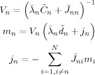(C5)

and is defined as in Eq. (C3) but is used instead of β. The subscripts in J _ni denote that part of J relevant to the nth and ith voxels. The quantities and are expectations that are defined in Eq. (50) of Penny et al. [2003]. The distribution over A can be re‐written as

(C6)

where m ${}_{\mathit{\text{v}}}^{\mathit{\text{T}}}$ = [m ${}_{\text{1}}^{\mathit{\text{T}}}$,m ${}_{\mathit{\text{n}}}^{\mathit{\text{T}}}$,..m ${}_{\mathit{\text{N}}}^{\mathit{\text{T}}}$] and V_v = (V ₁, V_n,…,V_N). This form of the posterior will be used in the derivation of KL‐divergences in Appendix E.

APPENDIX D: AVERAGE LIKELIHOOD

The average log‐likelihood for model m is given by

(D1)

where

(D2)

where ψ() is the digamma function [Press et al., 1992] and the quantity is defined in Eq. (77) of Penny et al. [2003]. This expression is identical to that given in Eq. (92) of Penny et al. [& 2003].

APPENDIX E: KL DIVERGENCES

Normal Densities

The multivariate Normal density is given by

(E1)

The KL divergence for Normal densities q(x) = (x; μ_q, Σ_q) and p(x) = (x; μ_p, Σ_p) is

(E2)

where |Σ_p| denotes the determinant of the matrix Σ_p.

Gamma Densities

The Gamma density is defined as

(E3)

For Gamma densities q(x) = (x; b_q, c_q) and p(x) = Ga(x; b_p, c_p) the KL‐divergence is

(E4)

where Γ() is the Gamma function [Press et al., 1992].

Precisions

For α, β and λ these divergences are straightforward to calculate as they reduce to a sum of KL‐divergences between gamma densities which have a known form and are computationally simple to evaluate.

(E5)

(E6)

(E7)

Regression Coefficients

For the regression coefficients, we have

(E8)

The only problematic term here is log | |. But we note that (i) H_w is a permutation matrix and so it will not affect determinants and (ii) if X is an m × m matrix and Y is an n × n matrix then (X ⊗ Y) = (X)ⁿ (Y)^m. We can therefore write

(E9)

We can also write

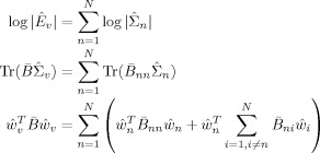(E10)

We can therefore write the divergence as a sum of ‘unique contributions’ from voxel n

(E11)

(E12)

The subscripts in B _ni denote that part of B relevant to voxels n and i.

AR Coefficients

For the AR coefficients, we can use the same approach

(E13)

Writing as a sum over ‘unique contributions’ from each voxel gives

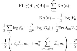(E14)

APPENDIX F: AR COEFFICIENTS WITH TISSUE‐TYPE PRIORS

AR Priors

We introduce the label s. For example s = {1,2,3} could correspond to grey matter, white matter and CSF. We also introduce the indicator function γ_ns which is 1 if voxel n belongs to category s and zero otherwise. N _s = ∑_s γ_ns is the number of voxels in the sth category. S is the number of categories. A ‘tissue‐type’ prior is then defined as

(F1)

where

(F2)

and a_s is the archetypal vector of AR coefficients for voxel type s, and β_s is the corresponding precision vector. This prior is like a Gaussian mixture model but one where the labelling is known.

In this paper, the parameters a_s and β_s are estimated from the data on a slice‐by‐slice basis. We use a Gamma prior on the precisions (see later section). For simplicity, there is no prior on a_s.

AR Posteriors

We have

(F3)

where

(F4)

and

(F5)

AR Precision Priors

We define the precision for the sth structure type and pth AR coefficient, β_sp, as the pth element of β_s. We then have

(F6)

AR Precision Posteriors

The posterior is given by

(F7)

(F8)

AR Means

The archetypal AR coefficient vectors are estimated using

(F9)

KL Divergences

(F10)

APPENDIX G: IMPLEMENTATION NOTE

The algorithm we have described is implemented in SPM version 5 and can be downloaded from SPM [2002]. Computation of a number of quantites (e.g. , and defined in appendices C and D) is now much more efficient than in previous versions [Penny et al., 2005]. These improvements are described in a separate document [Penny and Flandin, 2005]. To analyse a single session of data (e.g. the face fMRI data) takes about 30 minutes on a typical modern PC.

REFERENCES

- Ashburner J, Friston KJ ( 2003a): Image segmentation In: Frackowiak RSJ, Friston KJ, Frith C, Dolan R, Friston KJ, Price CJ, Zeki S, Ashburner J, Penny WD, editors. Human Brain Function, 2nd ed. Academic Press. [Google Scholar]
- Ashburner J, Friston KJ ( 2003b): Spatial normalization using basis functions In: Frackowiak RSJ, Friston KJ, Frith C, Dolan R, Friston KJ, Price CJ, Zeki S, Ashburner J, Penny WD, editors. Human Brain Function, 2nd ed. London: Academic Press. [Google Scholar]
- Auranen T, Nummenmaa A, Hammalainen M, Jaaskelainen I, Lampinen J, Vehtari A, Sams M ( 2005): Bayesian analysis of the neuromagnetic inverse problem with lp norm priors. Neuroimage 26(3): 870–884. [DOI] [PubMed] [Google Scholar]
- Beal M ( 2003): Variational algorithms for approximate Bayesian inference. PhD thesis, Gatsby Computational Neuroscience Unit, University College London.
- Beal M, Ghahraman Z ( 2003): The variational Bayesian EM algorithms for incomplete data: With application to scoring graphical model structures In: Bernardo J, Bayarri M, Berger J, Dawid A, editors. Bayesian Statistics 7. Cambridge University Press. [Google Scholar]
- Brett M, Anton JK, Valabregue R, Poline JB ( 2002): Region of interest analysis using an SPM toolbox. In: Eighth International Conference on Functional Mapping of the Human Brain, June 2–6, Sendai, Japan, 2002. Availabel on CD‐ROM in Neuroimage, Vol 16, No 2, abstract 497.
- Brett M, Penny WD, Kiebel SJ ( 2003): Introduction to random field theory In: Frackowiak RSJ, Friston KJ, Frith C, Dolan R, Friston KJ, Price CJ, Zeki S, Ashburner J, Penny WD, editors. Human Brain Function, 2nd ed. London: Academic Press. [Google Scholar]
- Box GEP, Tiao GC ( 1992): Bayesian Inference in Statistical Analysis. New York: Wiley. [Google Scholar]
- Buchel C, Friston KJ ( 1997): Modulation of connectivity in visual pathways by attention: Cortical interactions evaluated with structural equation modelling and fMRI. Cereb Cortex 7: 768–778. [DOI] [PubMed] [Google Scholar]
- Buckley MJ ( 1994): Fast computation of a discretized thin‐plate smoothing spline for image data. Biometrika 81: 247–258. [Google Scholar]
- Bullmore M, Brammer M, Williams S, Rabe‐Hesketh S, Janot N, David A, Mellers J, Howard R, Sham P ( 1996): Statistical methods of estimation and inference for functional MR image analysis. Magn Reson Med 35: 261–277. [DOI] [PubMed] [Google Scholar]
- Cover TM, Thomas JA ( 1991): Elements of Information Theory. Wiley. [Google Scholar]
- Frackowiak RSJ, Friston KJ, Frith C, Dolan R, Price CJ, Zeki S, Ashburner J, Penny WD ( 2003): Human Brain Function, 2nd ed. Academic Press. [Google Scholar]
- Friston KJ, Fletcher P, Josephs O, Holmes AP, Rugg MD, Turner R ( 1998): Event‐related fMRI: Characterizing differential responses. Neuroimage 7: 30–40. [DOI] [PubMed] [Google Scholar]
- Friston KJ, Glaser DE, Henson RNA, Kiebel SJ, Phillips C, Ashburner J ( 2002): Classical and Bayesian inference in neuroimaging: Applications. Neuroimage 16: 484–512. [DOI] [PubMed] [Google Scholar]
- Friston KJ, Holmes AP, Poline JB, Price CJ, Frith C ( 1995a): Detecting activations in PET and fMRI: Levels of inference and power. Neuroimage 40: 223–235. [DOI] [PubMed] [Google Scholar]
- Friston KJ, Holmes AP, Worsley KJ, Poline JB, Frith C, Frackowiak RSJ ( 1995b): Statistical parametric maps in functional imaging: A general linear approach. Hum Brain Mapp 2: 189–210. [Google Scholar]
- Gautama T, Van Hulle MM ( 2004): Optimal spatial regularisation of autocorrelation estimates in fMRI analysis. Neuroimage 23: 1203–1216. [DOI] [PubMed] [Google Scholar]
- Gelman A, Carlin JB, Stern HS, Rubin DB ( 1995): Bayesian Data Analysis. Boca Raton: Chapman and Hall. [Google Scholar]
- Henson RNA ( 2003): Analysis of fMRI time series In: Frackowiak RSJ, Friston KJ, Frith C, Dolan R, Friston KJ, Price CJ, Zeki S, Ashburner J, Penny WD, editors. Human Brain Function, 2nd ed. Academic Press. [Google Scholar]
- Henson RNA, Penny WD ( 2003): ANOVAs and SPM. Technical report, Wellcome Department of Imaging Neuroscience.
- Henson RNA, Rugg MD, Friston KJ ( 2001): The choice of basis functions in event‐related fMRI. Neuroimage 13( Suppl 1): 127. [Google Scholar]
- Henson RNA, Shallice T, Gorno‐Tempini ML, Dolan RJ ( 2002): Face repetition effects in implicit and explicit memory tests as measured by fMRI. Cereb Cortex 12: 178–186. [DOI] [PubMed] [Google Scholar]
- Kanwisher N, Stanley D, Harris A ( 1999): The fusiform face area is selective for faces not animals. Neuroreport 10: 183–187. [DOI] [PubMed] [Google Scholar]
- Kass RE, Raftery AE ( 1995): Bayes factors. J Am Stat Assoc 90: 773–795. [Google Scholar]
- Kiebel SJ ( 2003): The general linear model In: Frackowiak RSJ, Friston KJ, Frith C, Dolan R, Friston KJ, Price CJ, Zeki S, Ashburner J, Penny WD, editors. Human Brain Function, 2nd ed. Academic Press. [Google Scholar]
- Marchini J, Ripley B ( 2000): A new statistical approach to detecting significant activation in function MRI. Neuroimage 12: 168–193. [DOI] [PubMed] [Google Scholar]
- Marqui RP, Michel C, Lehman D ( 1994): Low resolution electromagnetic tomography: A new method for localizing electrical activity of the brain. Int J Psychophysiol 18: 49–65. [DOI] [PubMed] [Google Scholar]
- Miskin JW, MacKay DJC ( 2000): Ensemble learning for blind source separation In: Roberts SJ, Everson R, editors. ICA: Principles and Practice. Cambridge University Press. [Google Scholar]
- Neal RM, Hinton GE ( 1998): A view of the EM algorithm that justifies incremental, sparse, and other variants In: Jordan MI, editor. Learning in Graphical Models. Kluwer. [Google Scholar]
- Penny WD, Flandin G ( 2005): Bayesian analysis of single‐subject fMRI: SPM implementation. Technical report,Wellcome Department of Imaging Neuroscience.
- Penny WD, Kiebel SJ, Friston KJ ( 2003): Variational Bayesian inference for fMRI time series. Neuroimage 19(3): 727–741. [DOI] [PubMed] [Google Scholar]
- Penny WD, Stephan KE, Mechelli A, Friston KJ ( 2004): Comparing dynamic causal models. Neuroimage 22(3): 1157–1172. [DOI] [PubMed] [Google Scholar]
- Penny WD, Trujillo‐Barreto N, Friston KJ ( 2005): Bayesian fMRI time series analysis with spatial priors. Neuroimage 24: 350–362. [DOI] [PubMed] [Google Scholar]
- Press WH, Teukolsky SA, Vetterling WT, Flannery BVP ( 1992): Numerical Recipes in C. Cambridge: Cambridge University Press, UK. [Google Scholar]
- Sahani M, Nagarajan SS ( 2004): Reconstructing MEG sources with unknown correlations In: Saul L, Thrun S, Schoelkopf B, editors. Advances in Neural Information Processing Systems, Vol 16 Cambridge, MA: MIT. [Google Scholar]
- Sato M, Yoshioka T, Kajihara S, Toyama K, Goda N, Doya K, Kawato M ( 2004): Hierarchical Bayesian estimation for MEG inverse problem. Neuroimage 23: 806–826. [DOI] [PubMed] [Google Scholar]
- SPM ( 2002): Wellcome Department of Imaging Neuroscience. Available at http://www.fil.ion.ucl.ac.uk/spm/software/.
- Trujillo‐Barreto N, Aubert‐Vazquez E, Valdes‐Sosa PA ( 2004): Bayesian model averaging in EEG/MEG imaging. Neuroimage 21: 1300–1319. [DOI] [PubMed] [Google Scholar]
- Winer BJ, Brown DR, Michels KM ( 1991): Statistical Principles in Experimental Design. New York: McGraw‐Hill. [Google Scholar]
- Woolrich MW, Ripley BD, Brady M, Smith SM ( 2001): Temporal autocorrelation in univariate linear modelling of fMRI data. Neuroimage 14(6): 1370–1386. [DOI] [PubMed] [Google Scholar]
- Woolrich MW, Behrens TE, Smith SM ( 2004): Constrained linear basis sets for HRF modelling using Variational Bayes. Neuroimage 21: 1748–1761. [DOI] [PubMed] [Google Scholar]
- Worsley KJ, Liao CH, Aston J, Petre V, Duncan GH, Morales F, Evans AC ( 2002): A general statistical analysis for fMRI data. Neuroimage 15. [DOI] [PubMed] [Google Scholar]
- Zarahn E, Aguirre GK, D'Esposito M ( 1997): Empirical analysis of BOLD fMRI statistics 1. Spatially unsmoothed data collected under null‐hypothesis conditions. Neuroimage 5: 179–197. [DOI] [PubMed] [Google Scholar]