A Bayesian approach to determining connectivity of the human brain

Abstract

Recent work regarding the analysis of brain imaging data has focused on examining functional and effective connectivity of the brain. We develop a novel descriptive and inferential method to analyze the connectivity of the human brain using functional MRI (fMRI). We assess the relationship between pairs of distinct brain regions by comparing expected joint and marginal probabilities of elevated activity of voxel pairs through a Bayesian paradigm, which allows for the incorporation of previously known anatomical and functional information. We define the relationship between two distinct brain regions by measures of functional connectivity and ascendancy. After assessing the relationship between all pairs of brain voxels, we are able to construct hierarchical functional networks from any given brain region and assess significant functional connectivity and ascendancy in these networks. We illustrate the use of our connectivity analysis using data from an fMRI study of social cooperation among women who played an iterated “Prisoner's Dilemma” game. Our analysis reveals a functional network that includes the amygdala, anterior insula cortex, and anterior cingulate cortex, and another network that includes the ventral striatum, orbitofrontal cortex, and anterior insula. Our method can be used to develop causal brain networks for use with structural equation modeling and dynamic causal models. Hum Brain Mapp, 2005. © 2005 Wiley‐Liss, Inc.

INTRODUCTION

The central nervous system consists of billions of interconnected neurons and neuronal ensembles. These connections can exist intraregionally or can cross the entire brain. These intra‐ and interregional neuronal connections form the basis of neural processing in the human brain. Traditional activation studies focus on determining distributed patterns of brain activity associated with specific tasks. However, we can more thoroughly understand brain function by studying the interaction of distinct brain regions, as a great deal of neural processing is performed by an integrated network of several regions of the brain. Moreover, gaining a better understanding of these functional networks may also shed light on how different neurological illnesses or psychiatric disorders affect the brain.

Functional neuroimaging methods such as functional MRI (fMRI) allow us to examine relationships between spatially distinct regions of the human brain. These relationships can be described in terms of functional connectivity or effective connectivity. Friston et al. [1993] define functional connectivity as the “temporal correlations between spatially remote neurophysiological events” and effective connectivity as “the influence one neuronal system exerts over another.” Functional connectivity refers only to a relationship, or association, between two distinct brain regions. Effective connectivity, however, allows us to assess the degree of influence of one brain region over another.

One common approach used to determine effective connectivity of the brain is structural equation modeling (SEM) [McIntosh and Gonzalez‐Lima, 1994]. SEM takes advantage of changes in the covariances among neural elements to conduct a path analysis of a predefined anatomically connected regional brain network. SEM of functional neuroimaging data gives path coefficients between these predefined regions. The interpretation of the path coefficient for the path from brain region A to brain region B is the expected change in activity of region B given a unit change in region A [McIntosh and Gonzalez‐Lima, 1994]. One of the drawbacks of SEM is that it requires prior specification of a causal structural model that consists of a limited number of brain regions. McIntosh and Gonzalez‐Lima [1994] thus consider SEM to be a data‐driven, but hypothesis‐constrained, approach.

A more recent approach, developed explicitly for the analysis of functional imaging time series, is dynamic causal modeling (DCM) [Friston et al., 2003; Penny et al., 2004b]. In DCM the brain is treated as a deterministic nonlinear dynamic system that utilizes external stimuli to produce changes in brain activity. The measured responses are used to estimate model parameters that represent the effective connectivity between brain regions. A significant distinction between DCM and SEM is that DCM treats stimuli as known variables, whereas SEM treats the input as stochastic. Like SEM, however, DCM is used to test a specific predetermined hypothesis and is thus not an exploratory technique. By applying model selection [Penny et al., 2004a] and path analysis [Bullmore et al., 2000] techniques to DCM and SEM, functional connectivity analyses using DCM and SEM become somewhat more data‐driven, blurring the line between data and hypothesis‐driven approaches. (See Penny et al. [2004b] for a detailed comparison of SEM and DCM.)

We develop a purely data‐driven, hypothesis‐unconstrained approach which allows us to determine hierarchical functional brain networks based on functional connectivity and relative probabilities of elevated activity. Figure 1 presents a schematic illustration that conceptually describes a functional network of four brain voxels generically labeled w, x, y, and z. Although Figure 1 describes a network of only four voxels, we are able to apply our methodology to the set of all intracranial voxels. We use shading to denote a voxel exhibiting elevated activity (an elevated functional MR signal) and all connecting bars are potentially bidirectional. In our model we employ our fMRI data to construct a binary map that indicates whether each voxel exhibits elevated activity at a given time point. Voxels w and z become active together and inactive together; thus, we consider them as functionally connected, as sister voxels in the hierarchical network. Given some positive functional connectivity between voxel a and voxel b, if a exhibits elevated activity for a subset of the period in which b exhibits elevated activity, we consider b to be ascendant to a in the hierarchical network consisting of b and a. In Figure 1, while x, y, and w are functionally connected, voxels x and y exhibit elevated activity to a subset of the stimuli for which w exhibits elevated activity, suggesting that w is ascendant to x and y in our hierarchical functional network. w can be thought of as a central node in the network. It may also be possible to interpret ascendancy as a measure of influence, thus enabling our hierarchical functional networks to be used in modeling frameworks such as SEM and DCM.

Figure 1.

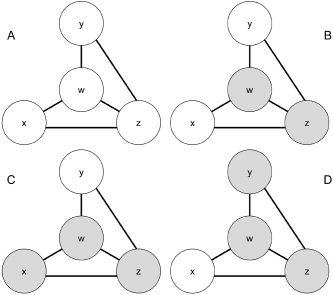
Functional network consisting of functionally connected brain voxels, w, x, y, and z. Shading for a given voxel indicates elevated activity. w and z are ascendant to x and y, thus x and y can be thought of as satellite voxels to the central voxels, w and z. A, B, C, and D represent different time points in the voxel time series of w, x, y, and z.

We develop a descriptive and inferential statistical method which makes use of this interpretation of joint and marginal activation probabilities of voxel pairs to determine two quantities: the amount of functional connectivity between two brain regions, and the degree of ascendancy over one another. We use a Bayesian approach, which allows us to account for anatomical relationships in the brain as well as known functional relationships from previous studies [Cordes et al., 2000; Hampson et al., 2002; Lowe et al., 1998; Xiong et al., 1999]. We are able to conduct posterior inference determining significant levels of connectivity and ascendancy by way of posterior probability maps (PPMs). Conducting inference with PPMs allows us to provide an upper bound on the rate of false discovery of significant functional connections [Friston and Penny, 2003]. We illustrate the use of our connectivity analysis using data from an fMRI study of social cooperation among women who played an iterated Prisoner's Dilemma game.

DATA

Iterated Prisoner's Dilemma Game

The iterated Prisoner's Dilemma game has been used in various disciplines to model social cooperation [Axelrod and Hamilton, 1981; Boyd, 1998; Nesse, 1990; Trivers, 1971]. Rilling et al. [2002] attempt to determine local brain regions that support the cognitive processes relating to cooperative, reciprocally altruistic relationships by examining regional brain activations with fMRI as subjects play the iterated Prisoner's Dilemma game with a partner outside the scanner. The iterated Prisoner's Dilemma problem involves two players who have the choice of either cooperating (C) with each other or defecting (D). We denote game outcomes in the format, XY, where X is the decision of player A and Y is the decision of player B. Depending on the decisions of both players, each receives a payoff proportional to the rewards shown in Table I. Results from the activation study conducted by Rilling et al. [2002] show that mutual cooperation is associated with consistent activation in brain regions linked to reward processing: nucleus accumbens, the caudate nucleus, ventromedial frontal/orbitofrontal cortex, and rostral anterior cingulate cortex.

Table I.

Prisoner's Dilemma payoff matrix

		Player A
		Cooperate	Defect
Player B	Cooperate	$2(2)	$3(0)
	Defect	$0(3)	$1(1)

Payoff to player A is the first number in each cell and the payoff to player B is in parentheses.

Experimental Design

Rilling et al. [2002] scan 17 female subjects (mean age = 23.8 years, range 20–30) after familiarizing them with the iterated Prisoner's Dilemma game. Each subject plays three sessions of the game. Each of the three sessions consists of 20–23 rounds of the Prisoner's Dilemma game. For the first 12 s of each round, the payoff matrix (Table I) is projected onto a screen that player A (inside the scanner) is able to see. The payoff to the player in the scanner is the first number in each cell and the payoff to the partner is in parentheses. Within the first 12 s of each game, players A and B both select whether to cooperate or defect. The partner's choice and game outcome is revealed 12 s after the game starts and is displayed for 9 s.

In two of the three sessions the player inside the scanner is told that their partner is a woman who they have previously met. In the remaining session, the player is told that their playing partner is a preprogrammed computer strategy. In fact, the playing partner for each of the three sessions is the same preprogrammed computer strategy that makes cooperate and defect choices according to predefined probabilities. (Refer to Rilling et al. [2002] for a more detailed description of the experimental design.)

Our data consists of 480 functional volumes for each of 17 subjects along with the decision and outcome for each subject and each round. There are four possible outcomes for a round: both players cooperate (CC), player A cooperates while player B defects (CD), player B defects while player A cooperates (DC), and both players defect (DD). The data for each voxel within a specific volume represents a surrogate measure of neural activity during that scan. We assume that the data for each voxel within a specific volume for a specific subject is normally distributed, which is a typical assumption for statistical modeling of fMRI data [Friston et al., 2002]. After convolution with a prespecified hemodynamic response function, our experimental design matrix for Subject 1 in our study takes the form shown in Figure 2. OCC‐ODD represent the game results during the first open‐ended (20–23 possible games) session, for which the subject was told her playing partner was a computer. HCC‐HDD represent the game results during the session when the player was told her partner was a human. CCC‐CDD represents the game results during the session when the player was correctly told that her partner was in fact a computer strategy.

Figure 2.

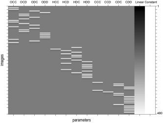
Design matrix for Subject 1. The first 12 columns represent experimental design covariates. The column labeled linear represents a linear detrending covariate.

Image Acquisition and Data Preprocessing

A 1.5 T Philips NT scanner is used to acquire T ₂‐weighted scans coronally with blood oxygen level‐dependent (BOLD) contrast. Rilling et al. [2002] acquire 27 slices, 6 mm in thickness, perpendicular to the anterior–posterior commissural line (repetition time = 3,000 ms, echo time = 28 ms, flip angle = 90°, 64 × 64 matrix). Functional images from each of three game sessions are collected sequentially with 1‐min intervening rest periods. A total of 480 volumes are collected for each of the 17 subjects. From here on, we let M equal the number of volumes per subject and S equal the number of subjects in the study.

We preprocess all of the data using SPM2 (http://www.fil.ion.ucl.ac.uk/spm/) by initially performing motion correction of images to the first functional scan within subject using a six‐parameter rigid body transformation and subsequently spatially normalizing the realigned images to the Montreal Neurological Institute (MNI) template by applying a 12‐parameter affine transformation followed by nonlinear warping using basis functions [Ashburner and Friston, 1999]. We bypass spatial smoothing to avoid further inducing nonneurophysiologically related spatial correlation.

METHODS

Determining Voxel Activation

We construct a general linear model which takes the form:

(1)

for each subject's voxel time series, where Y _M×1 is a column vector of the global mean adjusted functional MR signals for a single voxel [Friston et al., 1995]. The columns of X model the effects of interest, in this case the game outcome (CC, CD, DC, DD) for each of the three sessions, while the columns of H model confounding effects. K _M×p is a discrete cosine transform matrix with p harmonic periods up to, in our case, 62 s. K adjusts for possibly confounding low frequency trends in the data. W is a “pre‐whitening” matrix generated from an estimate of the matrix, V, of the intrinsic autoregressive correlation between ϵ_i and ϵ_j, where W′W = V ⁻¹ [Marchini and Smith, 2003]. Data from each voxel is pooled to generate a precise estimate of the serial correlations as we assume that V is the same at all voxels of interest. Because of this precision, we are able to assume that V is known [Kiebel and Holmes, 2003]. SPM2 assumes the form of V to be the first‐order autoregressive plus white noise model (AR(1)+wn) [Purdon and Weisskoff, 1998] and estimates the three hyperparameters of the covariance structure (two global parameters and one voxel‐wise parameter) by restricted maximum likelihood (ReML) [Kiebel and Holmes, 2003].

We define elevated activity in a voxel due to effects of interest by determining whether the data, adjusted for all known confounds exceeds a given threshold. Specifically, we denote R = WY − K − WH and define a vector of binary values for indicating whether elevated activity occurs for each scan, with respect to a constant c, by:

(2)

where σ² is the variance of W × ϵ. A is a column vector, where the mth element is 1 if the corresponding element of R is larger than c × σ; and the mth element of A is 0 otherwise. Our method defines a voxel as active if the associated level of activity is c standard deviations above what is expected under the null hypothesis that β = 0. Larger values of c identify voxels with more elevated levels of activity. We choose c = 1 when analyzing the Prisoner's Dilemma data.

We fit model (1) separately for all V voxels and for each of the S subjects. Let A _vsm be the indicator for elevated voxel activity as defined above for voxel v, subject s, and measurement m, and R _vsm indicate the corresponding level of activity. R _v indicates the entire time‐series for voxel v adjusted for all known confounds.

Bivariate Bernoulli Bayesian Model: A Dirichlet‐Multinomial Approach

We construct a bivariate Bernoulli Bayesian model for the joint activation of each pair of brain voxels using a multinomial likelihood with a Dirichlet prior distribution. The data we consider to model the joint activation probability for voxels a and b can be expressed as:

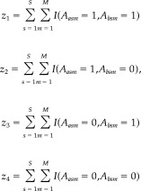(3)

for i = 1…4 and I(.) is the indicator function. z ₁ can be interpreted as the number of times that both a and b experience an elevated fMR signal over each scan of each subject. The multinomial likelihood of our data takes the form:

(4)

where the elements of θ are defined as:

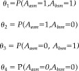(5)

for any subject s and measurement m. We assume each repeated measure on the same voxel pair is independent over time and across subjects.

Following a Bayesian formulation, we express our prior belief about θ by defining a Dirichlet prior which takes the form:

(6)

where all θ_i ≥ 0 and ∑${}_{\mathit{\text{i}}\text{= 1}}^{\text{4}}$θ_i = 1. Our posterior distribution, p(θ|z), is Dirichlet with parameters γ_i = α_i + z _i − 1 for i = 1…4.

Our interpretation of functional connectivity and the hierarchical nature of the connectivity (i.e., ascendancy) stems from Figure 1. As the relative difference between P(A _a|A _b) and P(A _a) increases and, conversely, the relative difference between P(A _b|A _a) and P(A _b) increases, the less independent and more functionally connected the two voxels are. Our functional connectivity metric allows us to determine ascendancy between a and b by the ratio of their respective marginal activation probabilities given significant functional connectivity between the two. Specifically, for two functionally connected voxels a and b, we say that a is ascendant to be whenever the marginal activation probability of a is larger than that of b. Our measure of functional connectivity suggests that voxels with vastly different probabilities of elevated activity can be functionally connected in the circumstance that one voxel becomes activated a subset of the time the other becomes active. Figure 3 illustrates these interpretations for three hypothetical voxel pairs (a ₁,b ₁), (a ₂,b ₂), and (a ₃,b ₃) for which the relative marginal activation probabilities are known. As the joint activation probability tends further from its expected value under independence, the functional connectivity grows larger. We utilize functions of the posterior probability distribution, p(θ|z), to determine the degree of functional connectivity between a voxel pair and the degree of ascendancy of one voxel on the other.

Figure 3.

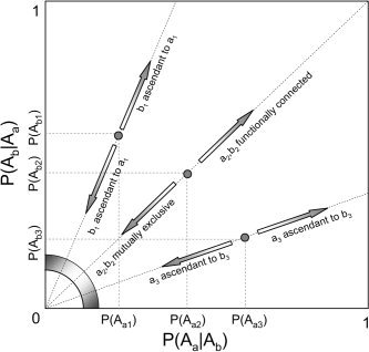
Three voxel pairs (a ₁,b ₁), (a ₂,b ₂), and (a ₃,b ₃) are illustrated, each with a different hierarchical relationship. As the slope of the line from the origin to (P(A _a),P(A _b)) gets further from 1, the degree of ascendancy between the voxel pair increases.

The hyperparameter, α_4×1, is a column vector that can be interpreted as a weight on θ_4×1. For the Prisoner's Dilemma study, we use the flat prior, α_4×1 = 0 _4×1, for each intracranial voxel pair. This suggests no prior information regarding the connectivity of any voxel pair and that any significant connectivity and ascendancy result is driven completely by the data.

Although we utilize flat priors in our analysis of the Prisoner's Dilemma data, it is possible to incorporate previously obtained functional or anatomical information through α. We provide a general outline in the Discussion regarding these alternative procedures for specifying α.

Descriptive and Inferential Methods

We describe the functional connectivity and ascendancy between each pair of brain voxels by functions of θ, which defines the joint distribution of elevated activity between two voxels, measured dichotomously. Our statistics are based on the interpretation of connectivity and ascendancy illustrated in Figure 3.

Functional connectivity

We develop a measure of association to describe functional connectivity based on the posterior distribution, p(θ|z), by considering a 2 × 2 table (Table II) with fixed marginal activation probabilities.

Table II.

Joint activation probabilities for voxels a and b

		Voxel a
		Active	Inactive
Voxel b	Active	θ1	θ3	θ1 + θ3
	Inactive	θ2	θ4	θ2 + θ4
		θ1 + θ2	θ3 + θ4	1

Existing measures of association for 2 × 2 tables, such as Cohen's Kappa [Cohen, 1960], do not treat the marginal totals as fixed, and are thus inappropriate to establish a measure of functional connectivity in our case. Cover and Thomas [1991] describe a measure which allows us to determine the mutual information, MI(a,b), between voxel pair (a,b); however, the problem of not considering fixed marginal totals remains. MI(a,b) may be relatively low in the case that a becomes active a subset of the time for which b is active. Our interpretation of this case would be a high functional connectivity with b ascendant to a.

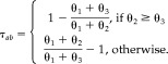
We formulate a new measure of association, κ, which ranges from −1 to 1, given a fixed pair of marginal activation probabilities. κ is defined as follows:

(7)

where E = (θ₁ + θ₂) (θ₁ + θ₃), max(θ₁) = min(θ₁ + θ₂, θ₁ + θ₃), min(θ₁) = max(0,2θ₁ + θ₂ + θ₃ − 1), and:

(8)

The numerator of κ measures the difference between the joint activation probability and the expected joint activation probability under independence, while the denominator is simply a weighted normalizing constant forcing κ to range from −1 to 1. min(θ₁ + θ₂, θ₁ + θ₃) represents the maximum value of P(A _a,A _b) given P(A _a) and P(A _b), while max(0,2θ₁ + θ₂ + θ₃ − 1) represents the minimum value of P(A _a,A _b) given P(A _a) and P(A _b). For two voxels that become active out of phase with each other, functional connectivity will be small, as κ considers joint activation probabilities as a measure of connectivity. Thus, a large κ between voxels a and b and between voxels b and c is not sufficient to demonstrate a connectivity between a and c, as is the case with a correlation approach [Stephan, 2004].

In contradistinction to Cohen's Kappa and its variants, given marginal activation probabilities of a and b, θ₁ + θ₂, and θ₁ + θ₃, respectively, our measure κ equals 1 when the joint activation probability of a and b, θ₁, is maximized. Thus, κ equals 1 when θ₂ or θ₃ equals 0. Conversely, κ equals −1 when θ₁ or θ₄ equals 0. κ satisfies the three key properties suggested by Piatetsky‐Shapiro [1991] for a measure of association:

• 1κ = 0 if voxels a and b are statistically independent.
• 2κ monotonically increases with P(A _a,A _b) as P(A _a) and P(A _b) remain fixed.
• 3κ monotonically decreases with P(A _a) when P(A _b) and P(A _a,A _b) remain fixed, and conversely, κ monotonically decreases with P(A _b) when P(A _a) and P(A _a,A _b) remain fixed.

We are able to obtain an estimate of p(κ|z) through sampling of the posterior Dirichlet distribution, p(θ|z). We conduct Bayesian inference on κ by estimating P(κ > e) > p, where e is a given effect size and p is a given probability cutoff. We estimate P(κ > e) > p by sampling from p(θ|z), calculating κ from each sample, and determining the proportion of samples for which κ > e.

Ascendancy

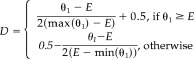
Given that voxels a and b are functionally connected (κ is significantly different from 0), we can interpret a measure of ascendancy based on the ratio of P(A _a) and P(A _b). Our measure of ascendancy, τ_ab, takes the following form:

(9)

τ_ab ranges from −1 to 1. Given κ ≠ 0, a positive value of τ_ab indicates that a is ascendant to b, while a negative value of τ_ab indicates that b is ascendant to a.

We are able to obtain an estimate of p(τ|z) by sampling from the posterior Dirichlet distribution, p(θ|z). We conduct Bayesian inference on τ by estimating P(τ > e) > p in a similar manner to the estimation of P(κ > e) > p.

RESULTS

Prisoner's Dilemma Results

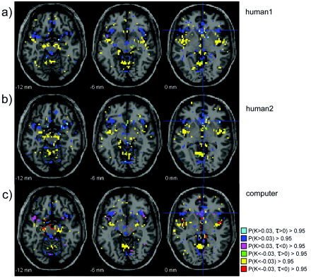
The Prisoner's Dilemma task is an interactive game that is expected to engage neural systems involved in social cognition [Adolphs, 2003]. In view of the amygdala's critical role in social cognition, the first seed is placed within the right amygdala (MNI coordinate 26, −1, −12). Our Prisoner's Dilemma experiment consists of three runs, two in which the participant is playing the game with presumed human playing partners and a third in which the participant is interacting with a computer partner. Given that subjects cooperate significantly more often with human partners [Rilling et al., 2002], we expect to observe similar patterns of connectivity for the two human runs and that these would, in turn, differ somewhat from the pattern observed for the computer run. For both human runs we observe strong positive connectivity between amygdala and anterior insula cortex (Fig. 4a,b), a region with which the amygdala has dense anatomical connections in monkeys [Stefanacci and Amaral, 2002] and which has shown activation in other social cognitive tasks [Sanfey et al., 2003; Winston et al., 2002]. Also of interest for both human runs is the negative connectivity with the rostral anterior cingulate cortex, an area implicated in emotion regulation [Davidson and Putnam, 2000] that may suppress amygdala activity. Only in the computer run (Fig. 4c) does a hierarchical relationship emerge between the amygdala, the anterior insula, and the rostral ACC, where the amygdala is ascendant to both the anterior insula and rostral ACC.

Figure 4.

Functional connectivity from seed placed in the right amygdala (MNI: 26 −1 −12).

A second seed is placed in the anteroventral striatum (MNI coordinates: 5, 18, 0), a region that uniquely activates to PD outcomes involving mutual cooperation with human partners [Rilling et al., 2002]. For all three runs this seed shows positive connectivity with orbitofrontal cortex (OFC) and anterior insula, and negative connectivity with posterior insula (Fig. 5). Positive connectivity with OFC is of interest given that OFC also activates in response to mutual cooperation in the PD game and, like the ventral striatum, receives midbrain dopamine projections involved in registering reward and reward prediction errors [Schultz, 1998]. The connectivity between ventral striatum and insula agrees with known anatomical connectivity data from monkeys [Haber and McFarland, 1999]. As for the amygdala seed, human and computer runs consistently differ in the pattern of hierarchy, with the computer run showing stronger ascendancy of amygdala over the insula. These differing patterns of ascendancy for human and computer runs are noteworthy, given that participants were significantly less likely to cooperate with computer vs. putative human partners, suggesting that they were adopting different psychological states in the two conditions. Overall, the validity of our method is attested to by the similarity of the results across the three separate runs, coupled with their agreement with anatomical connectivity data from monkeys and their compatibility with existing models of the neural bases of social cognition.

Figure 5.

Functional connectivity from seed placed in the anteroventral striatum (MNI: 5 18 0).

Simulation Results

We conduct a simulation study to analyze how well κ and τ can be determined for various signal‐to‐noise ratios (SNRs) and to compare our method to a traditional correlation approach. We simulate fMR data from four voxels by utilizing a single subject design matrix (Table II), X, from the prisoner's dilemma data. We assign the β parameters given in Table III to the four simulated voxels, w, x, y, and z, to create a simulated activation profile Y _i = Xβ_i + σ${}_{\mathit{\text{i}}}^{\text{2}}$, where β_i is the model parameter vector given in the row of Table III corresponding to voxel i and σ${}_{\mathit{\text{i}}}^{\text{2}}$ is i.i.d. N(0,σ²) noise. Y _i is thus a 480 × 1 vector. We assume that the voxel response is constant for each stimulus and for each voxel. We simulate the activation profile with various values of σ² to achieve three distinct SNRs where SNR is:

(10)

or the mean ratio of the mean signal (XB _i) of each of the four simulated voxels to the standard deviation of the white noise. We select an elevated activity cutoff level of c = 1 to determine κ and τ. To compare the variability of κ and correlation and to gain an understanding of how values of κ compare to the more well‐known correlation measure, we present correlation results as calculated by:

(11)

in Table IV.

Table III.

Activation profile for simulated voxels w, x, y, and z

	Stimulus
	OCC	OCD	ODC	ODD	HCC	HCD	HDC	HDD	CCC	CCD	CDC	CDD
w	1	1	1	1	1	1	1	1	1	1	1	1
x	0	0	0	1	0	0	0	1	0	0	0	1
y	0	0	1	0	0	0	1	0	0	0	1	0
z	0	1	1	1	0	1	1	1	0	1	1	1

We set the linear detrending parameter and intercept term to 0 for the purpose of simulation.

Table IV.

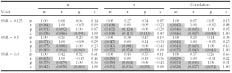
Means of κ, τ, and correlation over 1,000 simulations given in upper triangles

Corresponding standard deviations (std) in parentheses and given in lower triangles. κ_ij = κ_ji and τ_ij = −τ_ji for all i,j. std(κ_ij) = std(κ_ji) and std(τ_ij) = std(τ_ji) for all i,j.

From Table III we simulate a functional network such that w can be thought of as a central node, which is activated during any Prisoner's Dilemma game result. x is activated during each game where both players defect, while y activates for games where player A defects and player B cooperates. z activates for each result except when both players cooperate. Given our definitions of functional connectivity and ascendancy illustrated in Figure 3, w is ascendant to x, y, and z, while z is ascendant to x and y. z can be considered a satellite of a central node, w, and in turn, x and y can be considered satellites of z. Our results over 1,000 simulated activation profiles of the 4 voxels are given in Table IV. Connectivity results using simple correlation approach are also given in Table IV. Although our simulated network consists of only four voxels, our Prisoner's Dilemma data application constructs functional networks from the set of all intracranial voxels.

Voxels w and z have a mean κ of 0.61 when the SNR is 1.0, and the strength of the relationship appears to diminish as the SNR decreases. An ascendancy of w over z is revealed (τ = 0.11) when the SNR = 1.0 and this hierarchical relationship can be observed for all three SNRs. The means of τ are, in general, quite robust to changes in the SNR. The standard deviations of κ, τ, and correlation over the 1,000 simulation trials are given in the lower triangles of Table IV. As the SNR increases, the variability of each measure decreases at a similar rate. As could be expected, the standard deviations for κ are generally larger than the corresponding standard deviations for correlation as κ is calculated after dichotomization of the voxel time‐series. Our simulation results suggest that we are able to extract functional connectivity and ascendancy results for various SNRs.

DISCUSSION

We develop a purely data‐driven, hypothesis‐unconstrained approach which allows us to determine hierarchical functional brain networks based on functional connectivity and relative probabilities of elevated activity. We use a Bayesian approach that allows us to account for prior information on correlations between voxel pairs. We assess the relationship between a pair of voxels, a and b, in terms of two novel measures, κ and τ, which describe the functional connectivity and degree of ascendancy, respectively, between the voxels. κ is based on the joint bivariate distribution of probabilities of elevated activity between two voxels. The calculation of κ is based on the conditional activation probabilities P(A _a|A _b) and P(A _b|A _a) and the corresponding marginal distributions P(A _a) and P(A _b). We can interpret P(A _a|A _b) as the probability that a exhibits elevated activity given that b exhibits elevated activity after controlling for all known confounding effects. Given κ is significantly different from 0, i.e., a and b are functionally connected, τ indicates the degree of ascendancy between a and b by measuring the degree of dissimilarity between P(A _a) and P(A _b). In this manner, we are able to construct a hierarchical functional network consisting of central nodes, sister nodes, and satellite nodes, where central nodes are ascendant to satellite nodes and merely functionally connected to sister nodes. The interpretation of ascendancy and our hierarchical network structure as a directed graph of influence is appealing and can be tested by means of DCM and SEM. Interpretation of ascendancy as influence should be exercised with caution, as the conditional and marginal probability statements we consider do not directly imply physiological influence.

We specify a noninformative prior for the hyperparameter α in our analysis of the Prisoner's Dilemma data. Alternatively, one may incorporate prior functional or anatomical information into the selection of α. One approach defines α based on two measures: n _p, which determines the relative weight of the prior over the likelihood, and ρ_ab, a prior tetrachoric [Harris, 1988] correlation between the elevated activity indicators, A _a and A _b. Given the prior estimate of ρ_ab, e.g., from previous resting state fMRI studies [Cordes et al., 2000; Salvador et al., 2005], we can determine a prior estimate of the joint activation probability P(A _a,A _b) and finally α_ab. We know that:

(12)

Under a prior assumption that R _a and R _b are normally distributed with variance equal to 1, we can calculate ρ${}_{\mathit{\text{A}}{}_{\mathit{\text{a}}}\mathit{\text{aA}}{}_{\mathit{\text{b}}}}$ from its given tetrachoric correlation (see Appendix). We compute our prior parameters, α, from P(A _a), P(A _b), P(A _a,A _b), and n _p using the following expression:

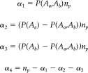(13)

A second approach is to incorporate anatomical information into the selection of α. We may proceed by a parameterization of the voxel‐pairwise correlations, ρ_ab = e ${}^{\text{− ϕ}\mathit{\text{d}}{}_{\mathit{\text{ab}}}}$, where ϕ is some positive constant and d _ab is a dissimilarity measure which depends on the type of brain tissue (cerebrospinal fluid, gray matter, white matter). These and other methods for specifying potentially informative priors represent an important area of future research.

The main focus of our method is the data‐driven construction of hierarchical functional brain networks via a Bayesian paradigm. However, an extension would be to consider an SEM consisting of the six brain regions identified by our analysis: the amygdala, anterior insula, posterior insula, rostral ACC, anteroventral striatum, and OFC. We can construct unidirectional SEM paths based on significant ascendancy among pairs of brain regions. For example, we would construct a path from the amygdala to the anterior insula and another from the amygdala to the rostral ACC for the structural equation model describing functional and effective connectivity in the case of an assumed computer partner. We would construct bidirectional paths based on brain regions discovered to be merely functionally connected. This approach to determining brain regions for SEM and DCM is not intended to supplant the standard psychophysiological interaction approach [Friston et al., 1997], but is merely a possible extension to our method.

The study of functional neural networks in the human brain is important to understand cognitive behavior. It may be the case that several brain regions work as a causal network to perform a task such as working memory, rather than a single brain region working independently. Analysis of the fluctuations in these causal networks may be an important tool needed to gain a better understanding of cognitive function. Comparing these causal networks under the same conditions across a normal subject group and a symptomatic subject group may also allow us to uncover new information about certain psychiatric disorders.

R _a and R _b are standard normal variables with correlation ρ. A _a = I(R _a > c) and A _b = I(R _b > c) where I(.) is the indicator function. Let ϕ(x) equal the standard normal cumulative distribution function, E(x) equal the expected value of x, and VAR(x) equal the variance of x.

(14)

(15)

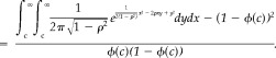(16)

REFERENCES

- Adolphs R (2003): Cognitive neuroscience of human social behaviour. Nat Rev Neurosci 4: 165–178. [DOI] [PubMed] [Google Scholar]
- Ashburner J, Friston KJ (1999): Nonlinear spatial normalization using basis functions. Hum Brain Mapp 7: 254–266. [DOI] [PMC free article] [PubMed] [Google Scholar]
- Axelrod R, Hamilton WD (1981): The evolution of cooperation. Science 211: 1390–1396. [DOI] [PubMed] [Google Scholar]
- Boyd R (1998): Is the repeated Prisoner's Dilemma a good model of reciprocal altruism? Ethol Sociobiol 9: 211–212. [Google Scholar]
- Bullmore E, Horwitz B, Honey G, Brammer M, Williams S, Sharma T (2000): How good is good enough in path analysis of fMRI data? Neuroimage 11: 289–301. [DOI] [PubMed] [Google Scholar]
- Cohen JA (1960): A coefficient of agreement for nominal scales. Educ Psych Meas 20: 37–46. [Google Scholar]
- Cordes D, Haughton VM, Arkanakis K, Wendt GJ, Turski PA (2000): Mapping functionally related regions of brain with functional connectivity MRI (fcMRI). Am J Neuroradiol 21: 1636–1644. [PMC free article] [PubMed] [Google Scholar]
- Cover TM, Thomas JA (1991): Elements of information theory. New York: John Wiley & Sons. [Google Scholar]
- Davidson RJ, Putnam KM (2000): Dysfunction in the neural circuitry of emotion regulation — a possible prelude to violence. Science 289: 591–594. [DOI] [PubMed] [Google Scholar]
- Friston KJ, Penny W (2003): Posterior probability maps and SPMs. Neuroimage 19: 1240–1249. [DOI] [PubMed] [Google Scholar]
- Friston KJ, Frith CD, Liddle PF, Frackowiak RS (1993): Functional connectivity: the principal component analysis of large (PET) data sets. J Cereb Blood Flow Metab 13: 5–14. [DOI] [PubMed] [Google Scholar]
- Friston KJ, Holmes AP, Poline J‐B, Grasby PJ, Williams SCR, Frackowiak RSJ, Turner R (1995): Analysis of fMRI time‐series revisited. Neuroimage 2: 45–53. [DOI] [PubMed] [Google Scholar]
- Friston KJ, Buechel C, Fink GR, Morris J, Rolls E, Dolan RJ (1997): Psychophysiological and modulatory interactions in neuroimaging. Neuroimage 6: 218–229. [DOI] [PubMed] [Google Scholar]
- Friston KJ, Penny W, Phillips C, Kiebel S, Hinton G, Ashburner J (2002): Classical and Bayesian inference in neuroimaging: theory. Neuroimage 16: 465–483. [DOI] [PubMed] [Google Scholar]
- Friston KJ, Harrison L, Penny W (2003): Dynamic causal modelling. Neuroimage 19: 1273–1302. [DOI] [PubMed] [Google Scholar]
- Haber SN, McFarland NR (1999): The concept of the ventral striatum in nonhuman primates. Ann N Y Acad Sci 877: 33–48. [DOI] [PubMed] [Google Scholar]
- Hampson M, Peterson BS, Skudlarski P, Gatenby JC, Gore JC (2002): Detection of functional connectivity using temporal correlations in MR images. Hum Brain Mapp 15: 247–262. [DOI] [PMC free article] [PubMed] [Google Scholar]
- Harris B (1988): Encyclopedia of statistical sciences, vol. 9 Tetrachoric correlation coefficient. New York: John Wiley & Sons; p 223–225. [Google Scholar]
- Kiebel S, Holmes A (2003): The general linear model In: Frackowiak RSJ, Friston KJ, Frith, Dolan R, Price CJ, Zeki S, Ashburner J, Penny WD, editors. Human brain function, 2nd ed. New York: Academic Press. [Google Scholar]
- Lowe MJ, Mock BJ, Sorenson JA (1998): Functional connectivity in single and multislice echoplanar imaging using resting state fluctuations. Neuroimage 7: 119–132. [DOI] [PubMed] [Google Scholar]
- Marchini JL, Smith SM (2003): On bias in the estimation of autocorrelations for fMRI voxel time‐series analysis. Neuroimage 18: 83–90. [DOI] [PubMed] [Google Scholar]
- McIntosh AR, Gonzalez‐Lima F (1994): Structural equation modeling and its application to network analysis in functional brain imaging. Hum Brain Mapp 2: 2–22. [Google Scholar]
- Nesse RM (1990): Evolutionary explanations of emotions. Hum Nat 1: 261–289. [DOI] [PubMed] [Google Scholar]
- Penny WD, Stephan KE, Mechelli A, Friston KJ (2004a): Comparing dynamic causal models. Neuroimage 22: 1157–1172. [DOI] [PubMed] [Google Scholar]
- Penny WD, Stephan KE, Mechelli A, Friston KJ (2004b): Modelling functional integration: a comparison of structural equation and dynamic causal models. Neuroimage 23: S264–S274. [DOI] [PubMed] [Google Scholar]
- Piatetsky‐Shapiro G (1991): Discovery, analysis and presentation of strong rules In: Piatetsky‐Shapiro G, Frawley WJ, editors. Knowledge discovery in databases. Cambridge, MA: MIT Press; p 2299–2248. [Google Scholar]
- Purdon P, Weisskoff R (1998): Effect of temporal autocorrelation due to physiological noise and stimulus paradigm on voxel‐level false positive rates in fMRI. Hum Brain Mapp 6: 239–249. [DOI] [PMC free article] [PubMed] [Google Scholar]
- Rilling JR, Gutman DA, Zeh TR, Pagnoni G, Berns G, Kilts C (2002): A neural basis for social cooperation. Neuron 35: 395–405. [DOI] [PubMed] [Google Scholar]
- Salvador R, Suckling J, Coleman MR, Pickard JD, Menon D, Bullmore E (2005): Neurophysiological architecture of functional magnetic resonance images of human brain. Cereb Cortex (in press). [DOI] [PubMed] [Google Scholar]
- Sanfey AG, Rilling JK, Aronson JA, Nystrom LE, Cohen JD (2003): The neural basis of economic decision‐making in the Ultimatum Game. Science 300: 1755–1758. [DOI] [PubMed] [Google Scholar]
- Schultz W (1998): Predictive reward signal of dopamine neurons. J Neurophysiol 80: 1–27. [DOI] [PubMed] [Google Scholar]
- Stefanacci L, Amaral DG (2002): Some observations on cortical inputs to the macaque monkey amygdala: an anterograde tracing study. J Comp Neurol 45: 301–323. [DOI] [PubMed] [Google Scholar]
- Stephan K (2004): On the role of general system theory for functional neuroimaging. J Anat 205: 443–470. [DOI] [PMC free article] [PubMed] [Google Scholar]
- Trivers R (1971): The evolution of reciprocal altruism. Q Rev Biol 46: 35–57. [Google Scholar]
- Winston JS, Strange BA, O'Doherty J, Dolan RJ (2002): Automatic and intentional brain responses during evaluation of trustworthiness of faces. Nat Neurosci 5: 277–282. [DOI] [PubMed] [Google Scholar]
- Xiong J, Parsons LM, Gao JH, Fox PT (1999): Interregional connectivity to primary motor cortex revealed using MRI resting state images. Hum Brain Mapp 8: 151–156. [DOI] [PMC free article] [PubMed] [Google Scholar]