

Abstract
The present work aims at analyzing the structure of cortical connectivity during the attempt to move a paralyzed limb by a group of spinal cord injured (SCI) patients. Connectivity patterns were obtained by means of the Directed Transfer Function applied to the cortical signals estimated from high resolution EEG recordings. Electrical activity were estimated in normals (Healthy) and SCI patients on twelve regions of interest (ROIs) coincident with Brodmann areas. Degree distributions showed the presence of few cortical regions with a lot of outgoing connections in all the cortical networks estimated irrespectively of the frequency band investigated. For both of the groups (SCI and Healthy), bilateral cingulate motor area (CMA) acts as hub transmitting information flows. The efficiency index, allowed to assert the ordered properties of such estimated cortical networks in both populations. The comparison of such estimated networks with those obtained from random networks, elicited significant differences (P < 0.05, Bonferroni‐corrected for multiple comparisons). A statistical comparison (ANOVA) between SCI patients and healthy subjects showed a significant difference (P < 0.05) between the local efficiency of their respective networks. For three frequency bands (theta 4–7 Hz, alpha 8–12 Hz, and beta 13–29 Hz) the higher value observed in the spinal cord injured population entails a larger level of internal organization and fault tolerance. This fact suggests a sort of compensative mechanism as local response to the alteration in their MIF areas, which is probably due to the indirect effects of the spinal injury. Hum Brain Mapp, 2007. © 2007 Wiley‐Liss, Inc.
Keywords: efficiency, degree distributions, digraph, DTF, high resolution EEG, spinal cord injured
INTRODUCTION
The concept of functional connectivity is viewed as central for understanding the organized behavior of anatomic regions in the brain during their activity. This organization is thought to be based on the interaction between different and differently specialized cortical sites. Cortical connectivity estimation aims at describing these interactions as connectivity patterns, which reflect direction and strength of the information flows between the cortical areas involved. In order to achieve this, several methods were applied on data gathered using both hemodynamic and electromagnetic techniques (Brovelli et al., 2004; Buchel and Friston, 1997; Gevins et al., 1989; Urbano et al., 1998). So far, the estimation of functional connectivity on EEG signals has been addressed by applying either linear or non‐linear methods which can both disclose the direct flow of information between scalp electrodes in time domain, although with different computational demands (Clifford, 1987; Inouye et al., 1995; Nunez, 1995; Stam and van Dijk, 2002; Tononi et al., 1994). In the latest years, a multivariate spectral technique called Directed Transfer Function (DTF) was proposed (Kaminski et al., 2001) to determine directional influences between any given pair of channels in a multivariate data set. This estimator is able to characterize at the same time direction and spectral properties of the brain signals, requiring only one multivariate autoregressive (MVAR) model to be estimated from all the EEG channel recordings. The DTF technique has been demonstrated (Kaminski et al., 2001) to rely on the key concept of Granger causality between time series (Granger, 1969), according to which an observed time series x(n) results in another series y(n), if the knowledge of x(n)'s past significantly improves prediction of y(n); if the relation between time series is not reciprocal, then x(n) may cause y(n), without y(n) necessarily yielding x(n). This lack of reciprocity provides the direction of the information flow between elements.
High Resolution EEG
Recently this multivariate method was applied to cortical waveforms estimated on realistic brain models by high resolution EEG recordings (Astolfi et al., in press; Babiloni et al., 2005). In fact, high resolution EEG techniques include the use of a large number of scalp electrodes, realistic models of the head derived from structural magnetic resonance images (MRIs) and advanced processing methodologies related to the solution of the linear inverse problem. These methodologies allow the estimation of cortical current density from sensor measurements (Grave de Peralta and Gonzalez Andino, 1999). Thus, functional connectivity estimation aims at describing brain interactions among several cortical areas with their direction and strength. The structure of these patterns allows us to treat them as real networks and to make some considerations about their topology by means of the graph theory.
Graph Theory
Since a graph is a mathematical representation of a network, which is essentially reduced to nodes and connections between them, a way to characterize topographical properties of real complex networks was proposed using a graph theoretical approach (Sporns et al., 2004; Strogatz, 2001; Wang and Chen, 2003). It was realized that functional connectivity networks estimated from EEG or magnetoencephalographic (MEG) recordings can be analyzed with tools that have been already generated for the treatments of graphs as mathematical objects (Stam, 2004). This is interesting since the use of mathematical indexes for summarizing some graph properties allows for the generation and the testing of particular hypotheses on the physiologic nature of the functional networks estimated from high resolution EEG recordings.
Small‐World Networks
Watts and Strogatz have shown that graphs with many local connections and few random long distance connections are characterized by a high cluster index C and a short path length L (Watts and Strogatz, 1998). Such near optimal models are designated as “small‐world” networks.
Many types of real networks have been shown to share these small‐world features (Strogatz, 2001). Patterns of anatomical connectivity in neuronal networks are particularly characterized by high clustering and a small path length (Watts and Strogatz, 1998). Networks of functional connectivity based upon fMRI BOLD signals or MEG recordings have also been shown to have small‐world features (Salvador et al., 2005; Stam, 2004). Recently, a more general setup has been tested in order to investigate real networks (Boccaletti et al., 2006). Global and local efficiency are similar to the path length and cluster index respectively, but they are more suitable for weighted and unconnected graphs. One of the advantages of the efficiency‐based formalism is that a single measure, the efficiency E (instead of the two different measures L and C used in the Watts‐Strogatz formalism), is sufficient to define the small‐world behavior (Latora and Marchiori, 2001).
Scale‐Free Networks
Besides, some real networks are mostly found to be very unlike the random graph in their degree distributions. It was demonstrated that such degree distributions follow a power law trend (Barabàsi and Albert, 1999). Those networks, called “scale‐free”, also exhibit the small‐world phenomenon, but tend to contain few nodes that act as highly connected “hubs”, although most of the nodes have low degrees. Scale‐free networks are very peculiar in how they respond to damages. An interesting characteristic of such networks is that they are extremely tolerant of random failures. In fact they can absorb random failures up to about 75% of their nodes before they collapse; however, they are more vulnerable to intentional attacks on their “hubs”. Attacks that simultaneously eliminate as low as about 18% of a scale‐free network's hubs can collapse the whole structure (Albert et al., 2000).
The use of graph tools seems to be particularly adequate to characterize functional connectivity patterns estimated with the DTF algorithm from high resolution EEG or MEG data. In particular, these tools were applied to a set of high resolution EEG data during the execution of a foot movement in a healthy population and during the attempt of the same movement in a group of spinal cord injured (SCI) patients. The question is whether the “architecture” of the functional connectivity in SCI patients, evaluated by graph analysis, may differ from healthy behavior. We wonder if SCI patients could show a more efficient cortical network in order to compensate the altered behavior of their primary motor areas because the spinal injury.
By using tools derived from graph theory, some indexes related to the topology of the cortical networks estimated were derived.
In particular, the main experimental questions investigated in this work are the following:
-
1
Is the efficiency index significantly different in the cortical connectivity networks estimated from normal and SCI subjects during the performance of the same task?
-
2
If it does exist, is such a difference dependent on the frequency contents of the cortical activity?
-
3
Are the efficiency values estimated in the two populations' networks different from those obtained in “random” graphs having the same dimensions?
METHODS
High Resolution EEG Recordings in SCI Patients and Healthy Subjects
All experimental subjects participating in the study were recruited by advertisement. Informed consent was obtained from each subject after the explanation of the study, which was approved by the local institutional ethics committee.
The healthy group consisted of five volunteers (age, 26–32 years; five males). They had no personal history of neurological or psychiatric disorder, were not taking medication, and were not abusing alcohol or illicit drugs.
The SCI group consisted of five patients (age, 22–25 years; two females and three males). Spinal cord injuries were of traumatic aetiology and located at the cervical level (C6 in three cases, C5 and C7 in two cases, respectively); patients had not suffered a head or brain lesion associated with the trauma leading to the injury.
For EEG data acquisition, subjects were comfortably seated on a reclining chair, in an electrically shielded, dimly lit room. They were asked to perform a brisk protrusion of their lips (lip pursing) while they were performing (healthy subjects) or attempting (SCI patients) the right foot movement.
The choice of this joint movement was suggested by the possibility to trigger the SCI patients' attempt at foot movement. In fact patients are not able to move their limbs; however they could move their lips. By attempting a foot movement associated with a lips protrusion, they provided an evident trigger after the volitional movement activity. Such a trigger has been recorded to synchronize the period of analysis for both the populations considered.
The task was repeated every 6–7 s, in a self‐paced manner, and the 100 single trials recorded were used for the estimate of functional connectivity by means of the Directed Transfer Function (DTF, see following paragraph). A 96‐channel system (BrainAmp, Brainproducts, Germany) was used to record EEG and EMG electrical potentials by means of an electrode cap and surface electrodes respectively. The electrode cap was built according to an extension of the 10‐20 international system to 64 channels. Structural MRIs of the subject's head were taken with a Siemens 1.5T Vision Magnetom MR system (Germany).
Cortical Activity and Functional Connectivity Estimation
Cortical activity from high resolution EEG recordings was estimated using realistic head models and cortical surface models with an average of 5,000 dipoles, uniformly disposed. Estimation of the current density strength, for each one of the 5,000 dipoles, was obtained by solving the Linear Inverse problem, according to techniques described in previous papers (Astolfi et al., in press; Babiloni et al., 2005). By using the passage through the Tailairach coordinates system, twelve Regions Of Interest (ROIs) were then obtained by segmentation of the Brodmann areas (B.A.) on the accurate cortical model utilized for each subject. Bilateral ROIs considered in this analysis are the primary motor areas for foot (MIF) and lip movement (MIL), the proper supplementary motor area (SMAp), the standard pre‐motor area (BA6), the cingulated motor area (CMA) and the associative area (BA7). As an example for the different steps involved in the generation of the high resolution EEG model employed in this study, Figure 1 presents a superimposition of the electrode montage with actual head structures as well as the cortical areas employed as regions of interest.
Figure 1.
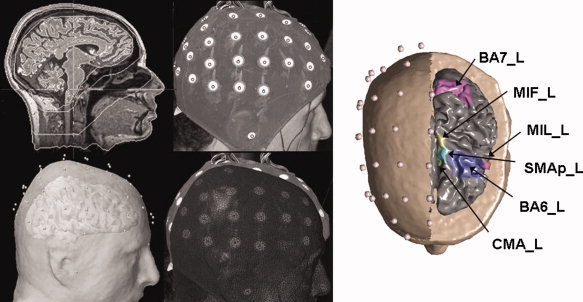
Left: Four steps involved in the generation of the Lead Field matrix for the estimation of cortical current density from EEG recordings. From left to right, from top to the bottom: MRI images from a healthy subject, generation of the head models and superimposition with electrodes cap. On the right of the figure the Regions of Interest (ROIs), taken into account for successive connectivity estimations, are illustrated. Cortical activity was estimated on the cortical areas of interest from the high resolution EEG recordings performed in both the populations. [Color figure can be viewed in the online issue, which is available at www.interscience.wiley.com]
For each EEG time point, the magnitude of the 5,000 dipoles composing the cortical model was estimated by solving the associated Linear Inverse problem (Grave de Peralta and Gonzalez Andino, 1999). Then average activity of dipoles within each ROI was computed. In order to study the preparation for an intended foot movement, a time segment of 1.5 s before the lips pursing was analyzed; lips movement was detected by means of an EMG.
Although motor responses could be analyzed at the same way, we would concentrate on the “intention‐to‐move” time interval in order to have results that could be used successively in the Brain Computer Interface context. BCI is a recent field of research in which brain signals related to movement intention can be suitably treated to control external devices. This fact would improve the condition of SCI patients in a next future.
Resulting cortical waveforms, one for each predefined ROI, were then simultaneously processed for the estimation of functional connectivity by using the Directed Transfer Function. DTF is a full multivariate spectral measure, used to determine the directed influences between any given pair of signals in a multivariate data set (Kaminski et al., 2001). In order to be able to compare the results obtained for data entries with different power spectra, the normalized DTF was adopted. It expresses the ratio of influence of element j to element i with respect to the influence of all the other elements on i. Equations used for the implementation of the DTF applied on data analysis are described in previous papers (Astolfi et al., 2005; Babiloni et al., 2005). Application of this method to the ROIs waveforms returns a cortical network for each frequency band of interest: (theta 4–7 Hz, alpha 8–12 Hz, beta 13–29 Hz, 30–40 Hz). Only estimated DTF connections that are statistically significant (at P < 0.001) after a contrast with the surrogate distribution of DTF values on the same ROIs obtained with a Montecarlo procedure were considered for the network to be analyzed with graph theory's tools. This procedure enables us to consider only those functional links that are not due to chance.
As an example of the networks estimated for the two populations analyzed, Figure 2 shows the average cortical network estimated in the beta frequency band for the SCI group and for the healthy group during the motor attempt/execution of the task. The Figure shows the average intensity of 30% of the greater connections belonging to two experimental subjects at least. The cortex of one particular subject was used for display purposes, being the computations performed on the realistic ROIs of each individual cortex. One arrow from the cortical region X to the cortical region Y describes the existence of a stable causal relation between them. Estimated cortical waveform in the X region “Granger”‐causes the estimated cortical waveform in the Y region, in the particular frequency range.
Figure 2.
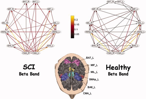
Average connectivity networks among ROIs, for SCI group (upper left) and healthy group (upper right), obtained from DTF in the Beta frequency band during the foot‐lip task. They show the 30% of the most powerful edges. Only edges shared by at least two experimental subjects are shown. Nodes follow the disposition of ROIs on the cortex, represented at the bottom of the figure. Head is seen from above, with nose towards the bottom of the page; left hemisphere is on the right part of the figure. Flows direction is represented by an arrow, while intensity is coded by its color and size. Each node is labeled with the ROI acronym. [Color figure can be viewed in the online issue, which is available at www.interscience.wiley.com]
Graph Analysis
Application of graph theory to small networks is rather new when compared to standard application of such theory in biological context. However, recently the need for the use of graph analysis applied to small networks has been underlined (Hilgetag et al., 2000; Stam et al., 2006a, b). Although application of graph theory to 28 raw EEG signals has been already addressed (Micheloyannis et al., 2006), we underline that achieving cortical waveforms allows the possibility to represent nodes as particular Brodmann areas of the cortex (Babiloni et al., 2005). The use of raw EEG signals, in the context of graph theory, returns less powerful results since nodes within the network represent electrodes on the scalp, which could have indirect links with the cortical areas beneath them.
In order to achieve topological features, a cortical network has to be converted into a directed unweighted graph (digraph). In this study, connection matrix contains DTF values for each directed pair of ROIs and can be converted to an adjacency matrix A by considering a threshold T that represents the number of the most powerful connections to be considered. If the number of links in the DTF matrix exceeds T, less powerful connections will be removed until that threshold is reached. Also, T can be expressed as connection density, that is, the ratio between the number of all the effective connections and the number of all possible connections within the graph. In order to study the topology of the networks at different connection densities or costs (Latora and Marchiori, 2003), a range of values (0.1, 0.15, 0.2, 0.25, 0.3, 0.35, 0.4, 0.45, 0.5) was explored.
Once the cortical network has been converted, it is possible to characterize the digraph in terms of its degrees, degree distributions, global, and local efficiency.
Degrees and Distributions
The simpler attribute for a graph's node is its degree of connectivity, that is, the total number of connections with other nodes. The arithmetical average of all node's degree 〈k〉 is called mean degree of the graph. Indeed, this mean value gives little information about the behavior of degree within the system. Hence, it is useful to introduce P(k), the fraction of vertices in the graph that have degree k. Equivalently, P(k) is the probability that a vertex chosen uniformly at random has degree k. A plot of P(k) for any given network can be constructed by making a histogram of the degrees of vertices. This histogram is the degree distribution for the graph and it allows better understanding of the degree allocation in the system. Here, because the graph is directed, the in‐degree k in and the out‐degree k out for each node must be considered separately. They represent the total number of connections incoming (afferent) to a vertex and outgoing (efferent) from the same vertex, respectively. Degrees have obvious functional interpretations. A high degree‐in indicates that a neural region is influenced by a large number of other areas, while a high degree‐out indicates a large number of potential functional targets. For large networks both distributions P in (k) and P out (k) over the entire digraph may be inspected for scale‐free attributes such as power laws (Albert and Barabási, 2002). Besides, contrasting biological degree distributions with those obtained from same‐sized random digraphs could reveal interesting differences.
Efficiency
Efficiency is a quantity recently introduced (Latora and Marchiori, 2001) to measure how efficiently the nodes of the network communicate when they exchange information in parallel.
It is computed from the distance matrix D, which contains distances between each pair of nodes, defined as the length of the shortest path between them (Harary, 1969); if there is no path linking a pair of vertices, the distance is infinite. Computationally, D can be determined using several algorithms with different time complexity. Here, the Floyd‐Warshall algorithm (1962), which computes for each pair of vertices the minimum weight among all paths between the two vertices, was applied.
The efficiency eij in the communication between vertices i and j can then be defined to be inversely proportional to their shortest distance: eij = 1/dij. When there is no path in the graph between i and j, dij = ∞ and consistently, eij = 0.
Global efficiency of A can be defined as
| (1) |
where N is the number of vertices composing the graph. Note that 1/L (inverse of the characteristic path length) can be seen as first approximation of E glob.
Since efficiency is also defined for disconnected graphs, the local properties of A can be characterized by evaluating for each vertex i the efficiency of A i, the sub‐graph of the neighbors of i. Local efficiency is the average of all the sub‐graphs' global efficiencies:
| (2) |
This quantity plays a role similar to that of the clustering coefficient C, previously used in literature. Since node i does not belong to the sub‐graph A i, local efficiency E loc reveals how much the system is fault‐tolerant; thus it shows how efficient the communication is between the first neighbors of i when i is removed.
The definition of small‐world can now be rephrased and generalized in terms of the information flow: small‐world networks have high E glob and E loc, that is, they are very efficient in global and local communication. This definition is valid both for unweighted and weighted graphs, and can also be applied to disconnected or non‐sparse graphs or both.
Contrast Between Groups
Analysis of variance (ANOVA) was used in order to find significant differences between the indices of efficiency computed in the two populations for all the frequency bands. ANOVA was chosen since it is known to be robust with respect to the departure of normality and homoscedasticity of data being treated (Zar, 1984). Separate ANOVAs were conduced for each of the two variables E glob and E loc, computed in each frequency band relevant for this study. Statistical significance was put at 0.05 and main factors of the ANOVAs were the “between” factor GROUP (with two levels: SCI and Healthy) and the “within” factor BAND (with four levels: theta, alpha, beta, and gamma). Greenhouse and Geisser correction was used for the protection against the violation of the sphericity assumption in the repeated measure ANOVA. Besides, post‐hoc analysis with the Duncan's test and significance level at 0.05 was performed. All the statistical analysis was performed with the software Statistica©, StatSoft, Inc.
Contrast With Random Graphs
The contrast between functional networks obtained from the two experimental groups and random digraphs having the same number of nodes and connections of the cortical networks was investigated. These graphs were generated distributing a fixed number of connections between randomly chosen couple of nodes (Latora and Marchiori, 2003). A set of 1,000 random digraphs was collected and the respective distributions of global and local efficiency values were calculated. A hypothesis testing procedure was employed in order to detect significant differences between average values of the random digraphs and average values of the experimental digraphs. The large amount of random values assures the normality of their distributions, then it was separately performed a z‐test for each average value of global and local efficiency gathered from the two populations in each frequency band.
Significance level was posed at 0.05 (Bonferroni corrected for multiple comparisons) and it was determined whether an average value obtained from an experimental group in a particular band, could belong to a normal distribution of 1,000 values with a known standard deviation.
RESULTS
All results displayed are relative to networks with a threshold applied equals to 0.3. This means that all digraphs analyzed have the same number of connections representing the 30% of the most powerful links within the network. This particular value represents the median of an interval of thresholds (from 0.1 to 0.5, see Graph Analysis) for which results remain significantly stable. In all the networks investigated, values of degrees for each node increase or decrease proportionally to the threshold selected. Thus all differences among graphs' degrees are maintained.
Moreover, according to the previous description in Contrast Between Groups, global and local efficiency of the two populations for each of the following thresholds were statistically compared. It has been seen that the only significant (P < 0.05) differences were due to local efficiency in a sub‐interval ranging from 0.2 to 0.4. The stability of results is then clear in a range of ±10% around the chosen value. Trends of average local efficiencies at different values of threshold in the two experimental populations for a representative frequency band, are shown in Figure 3.
Figure 3.
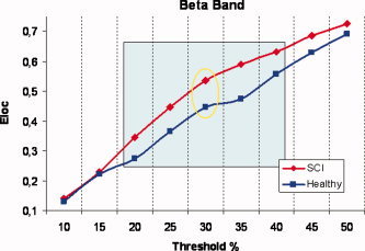
Average values of local efficiency at different values of threshold in the two experimental populations for the representative beta frequency band. Red line represents values for SCI networks while blue line refers to Healthy networks. The square inside displays the sub‐interval of thresholds for which E loc remains significantly (P < 0.05) different between the two groups. Yellow ellipse localizes the threshold used (30%) in order to illustrate all following results. [Color figure can be viewed in the online issue, which is available at www.interscience.wiley.com]
Degrees
Figure 4 shows results relative to the average incoming connections (in‐degree) and the average outgoing connections (out‐degree) for the ROIs of the SCI population in four different frequency bands analyzed. Level of involvement has to be considered separately for incoming connections and outgoing connections. Contrast between degrees “in” and “out” of the normal population, during the preparation to the movement execution, is presented in Figure 5.
Figure 4.
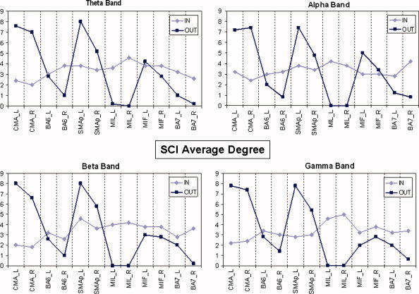
Average degrees of SCI group in the frequency bands analyzed. Light blue line represents degree‐in, while dark blue refers to degree‐out. On the abscissas ROIs label are displayed; on the ordinates there are degree values. [Color figure can be viewed in the online issue, which is available at www.interscience.wiley.com]
Figure 5.
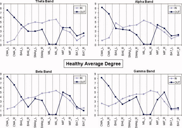
Average degrees of the healthy group in all the frequency bands analyzed. Same conventions than in Figure 4. [Color figure can be viewed in the online issue, which is available at www.interscience.wiley.com]
Direct comparisons of the data presented in Figures 4 and 5 show that for all the frequency bands there is a strong involvement of SMAp areas in SCI population during the attempt to move the paralyzed limb, which is not so evident in the healthy subjects. The absolute level of incoming connections in each single ROI seems rather similar in the two populations. Anyway some differences appear in BA7 areas, where in‐degree is higher in the SCI group irrespectively of the frequency band.
The number of outgoing connections for cingulate motor areas (CMA) is very high for both of the two experimental groups, while no connections seem to come from the primary motor areas of the lips (MIL). In particular, in the beta frequency band, healthy subjects present a remarkable flow coming from their primary motor areas (MIF), while a large number of links in the SCI patients come out from the SMAp areas.
Degree Distributions
As outlined in the Methods section, mean degrees are just indicative of the global behavior of a digraph's connectivity. For a more detailed analysis, it is necessary to compute two degree distributions P in and P out for each of the networks obtained. At the top of Figure 6 average trends of the degree distributions are shown for SCI and Healthy groups, in a representative frequency band. Histogram values were normalized to the size of the digraph, which is the number of the elements within the network (12 ROIs). An interesting result is that in‐degree and out‐degree distributions show different trends within each group. Right‐skew tails of out‐degree distribution indicates the presence of few nodes with a very high level of outgoing connections, while for the in‐degree distribution there are no ROIs in the network with more than six (seven in some other bands) incoming connections.
Figure 6.
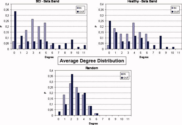
Average trends of degree distributions are shown for SCI (upper‐left) and healthy (upper‐right) group in the beta frequency band. In‐degree distribution P in is represented by light blue bars, while dark blue bars refer to out‐degree distribution P out. In order to have comparable results the histogram values were normalized to the number of the elements within the network (12 ROIs). Average degree distributions of five random digraphs, are shown in the bottom part of the Figure with the same previous conventions. [Color figure can be viewed in the online issue, which is available at www.interscience.wiley.com]
This unsettling, found in each of the two experimental groups and frequency band, is an attribute of the real networks that cannot be observed in random graphs. At the bottom of Figure 6, average degree distributions obtained from a set of five random digraphs are shown; it is evident the absence of “hubs” either for efferent and afferent flows.
Contrast Between Groups
In order to catch inter‐individual variance of the results, values of indexes employed (E glob, E loc) were computed for cortical networks estimated on each experimental subject (spinal cord injured and healthy), in the four frequency bands.
Average values of the SCI and healthy population are then reported in the Figures 7 and 8 respectively, in the four frequency bands.
Figure 7.
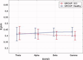
Average values of global efficiency (E glob) for the levels of “within” factor BAND, grouped by SCI and healthy subjects. No statistically significant differences were found between normal subjects and SCI patients. Vertical bars denote 0.95 confidence intervals. [Color figure can be viewed in the online issue, which is available at www.interscience.wiley.com]
Figure 8.
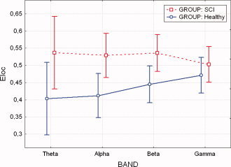
Average values of local efficiency (E loc) for the levels of “within” factor BAND, grouped by SCI and Healthy subjects. A statistically significant difference (P < 0.05) was noted between normal subjects and SCI patients. Vertical bars denote 0.95 confidence intervals. [Color figure can be viewed in the online issue, which is available at www.interscience.wiley.com]
Successively, a contrast between values of the two populations was addressed by using the Analysis of Variance (ANOVA), as summarized below.
Global efficiency
ANOVA performed on the E glob variable showed no significant differences for the main factors GROUP and BAND. In particular “between” factor GROUP was found having an F value of 0.83, P = 0.392 while the “within” factor BAND was found having an F value of 0.002 and P = 0.99.
Local efficiency
ANOVA performed on the E loc variable revealed a strong influence of the between factor group (F = 32.67, P = 0.00045); while the BAND factor and the interaction between GROUP X BAND were found not significant (F = 0.21 and F = 0.91 respectively, P values equal to 0.891 and 0.457).
Post‐hoc tests revealed a significant difference between the two examined experimental groups (SCI, Healthy) in theta, alpha, and beta band (P = 0.006, 0.01, 0.03 respectively). It can be observed (Fig. 8) that the average values of the local efficiency in the SCI subjects are significantly higher than those obtained in the Healthy group, for the three frequency bands.
Contrast With Random Graphs
Figure 9 shows the contrast between the values obtained for global and local efficiency in the two populations studied with those obtained in a set of 1,000 random digraphs, having the same number of nodes and arcs.
Figure 9.
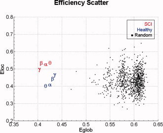
Scatter plot of global and local efficiency. All the average values are grouped by SCI patients (red symbols) and healthy subjects (blue symbols) while black dots represent the distribution of 1000 random digraphs. Greek symbols characterize the frequency bands involved in the study. [Color figure can be viewed in the online issue, which is available at www.interscience.wiley.com]
To state the statistical significance of the differences observed in the mean values of those indexes, separate z‐tests, at the significance level of 0.05 (Bonferroni‐corrected for multiple comparisons), were performed and are summarized in the Table I.
Table I.
z‐Values of the 16 contrasts performed with a z‐test with significance level at 0.05 (Bonferroni‐corrected for multiple comparisons)a
| z‐values | SCI‐theta | SCI‐alpha | SCI‐beta | SCI‐gamma | Healthy‐theta | Healthy‐alpha | Healthy‐beta | Healthy‐gamma |
|---|---|---|---|---|---|---|---|---|
| E glob | 237.45 | 250.13 | 262.88 | 267.07 | 249.81 | 238.21 | 225.95 | 223.4 |
| E loc | −57.714 | −53.314 | −57.025 | −38.936 | 15.99 | 11.051 | −7.163 | −21.674 |
All contrasts were significant (P < 0.001); so respective percentiles are not reported. Positive/negative z‐values indicate that the mean value of the random distribution is higher/lower than the average value of an experimental group in a particular frequency band.
Results show that for both of the experimental groups (SCI and healthy) and in all the frequency bands employed, global efficiency is significantly lower than the random mean value. Instead, local efficiency for the SCI group in every band is significantly higher than the random one. The same behavior appears for the healthy population in each frequency band except for theta and alpha that contrarily show lower values of local efficiency when compared with the random distribution.
DISCUSSION
The possibility to adopt a mathematical approach notably improves the capability of detecting relevant features in real complex networks. In this sense, graph theory can help the analysis of connectivity patterns estimated from high resolution EEG by means of MVAR methods.
Analysis performed on the cortical networks estimated from the group of normal and SCI patients revealed that both groups present few nodes with a high out‐degree values. This property is valid in the networks estimated for all the frequency bands investigated. In particular, cingulate motor areas (CMAs) ROIs act as “hubs” for the outflow of information in both groups, SCI and healthy. This means that removal of CMAs from the estimated patterns will cause a collapsing of the whole cortical network, thus corrupting the characteristic behavior of the preparation to the effecting of this experimental task. In addition, while SCI patients show a remarkable flow outgoing from their SMAp areas in the beta frequency band, healthy subjects show a relevant outflow from the MIF areas in the same frequency band.
Although the presence of “hubs” in the out‐degree distributions of all the cortical digraphs could suggest a power‐law trend, we cannot formally assert their scale‐free properties, according to actual procedures (Boccaletti et al., 2006), because the small size of the networks involved prevents us from achieving a reliable degree distributions.
Results suggest that spinal cord injuries affect the functional architecture of the cortical network sub‐serving the volition of motor acts mainly in its local feature property. In fact, SCI patients have shown significant differences from healthy subjects in this index; this could be due to a functional reorganization phenomenon, generally known as brain plasticity (Raineteau and Schwab, 2001). The higher value of local efficiency E loc suggests a larger level of the internal organization and fault tolerance (Sivan et al., 1999). In particular, this difference can be observed in three frequency bands, theta, alpha and beta, which are already known for their involvement in electrophysiologic phenomena related to the execution of foot movements (Pfurtscheller and Lopes da Silva, 1999). A high local efficiency implies that the network tends to form clusters of ROIs which hold an efficient communication. These efficient clusters, noticed in the SCI group, could represent a compensative mechanism as a consequence of the partial alteration in the primary motor areas (MIF) due to theeffects of the spinal cord injury. Instead, it seems that the global level of integration between the ROIs within the network do not differ significantly from the healthy behavior. This could mean that spinal cord injuries do not affect the global efficiency of the brain which attempts to preserve the same external properties observed during the foot‐lip task in the cortical networks of healthy subjects.
By perusing data presented in both Table I and Figure 9, it is clear that cortical networks estimated in this study are not structured like random networks. Instead, well ordered properties arise from most of the digraphs obtained from each experimental group and frequency band. In fact, they show similar values of global and local efficiency and more precisely fault tolerance is privileged with respect to global communication. These results indicate that cortical networks behave globally in the same way as they behave locally. Moreover, these real digraphs show a lower global efficiency and a higher local efficiency than respective values obtained from random digraphs. This fact suggests during the experimental task brain networks tend to follow an ordered spatial topology rather than a small‐world or a random architecture. Here, random digraphs are generated with the same number of nodes and edges of the connectivity patterns obtained. Anyway, in order to have more robust comparisons algorithms that also preserve the degree distributions are available and recently applied to cortical networks (Sporns and Zwi, 2004).
Theoretical graph approach can be a very useful tool, able to catch some global and local features in the functional connectivity patterns estimated from the high resolution EEG. Degrees together with their distributions, global and local efficiency, point out some aspects in the structure of cortical network that cannot be easily noticed and that allow comparison of different networks between different task or subjects. In addition, appropriate algorithms that also take into account the actual values of connectivity strengths estimated by the DTF procedures could be adopted, in order to further increase the efficacy of the analysis proposed (Latora and Marchiori, 2003).
On the basis of these experimental results obtained from the application of graph theory tools to the functional connectivity networks estimated by using advanced high resolution EEG and DTF algorithms, we have possible answers to the experimental questions posed in the introduction section.
In particular:
-
1
It seems that there are significant differences in the cortical functional connectivity networks between SCI patients and healthy subjects. Such differences are related to the internal organization of the network and its fault tolerance, which in SCI patients appears to be higher than in normal subjects, as suggested by the significant increase of the local efficiency.
-
2
Differences in this functional connectivity networks are higher in the theta, alpha and beta frequency bands, which are already known to be involved in the phenomena related to the execution of motor acts.
-
3
All functional connectivity networks extracted from the two experimental groups showed ordered properties and significant differences from “random” networks having the same characteristic sizes.
In conclusion, graph analysis tools described here seem to be instruments that are adequate to study distinctive features of functional connectivity networks, estimated with the use of advanced high resolution EEG methodologies.
Acknowledgements
This work reflects only the authors' views; funding agencies are not liable for any use that may be made of the information contained herein.
REFERENCES
- Albert R,Barabasi A ( 2002): Statistical mechanic of complex networks. Rev Mod Phys 74: 47–97. [Google Scholar]
- Albert R,Jeong H,Barabasi A ( 2000): Error and attack tolerance of complex networks. Nature 406: 378–382. [DOI] [PubMed] [Google Scholar]
- Astolfi L,Cincotti F,Mattia D,Babiloni C,Carducci F,Basilisco A,Rossini PM,Salinari S,Ding L,Ni Y,He B,Babiloni F ( 2005): Assessing cortical functional connectivity by linear inverse estimation and directed transfer function: Simulations and application to real data. Clin Neurophysiol 116: 920–932. [DOI] [PubMed] [Google Scholar]
- Astolfi L,Cincotti F,Mattia D,Marciani MG,Baccalà L,De Vico Fallani F,Salinari S,Ursino M,Zavaglia M,Ding L,Edgar JC,Miller GA,He B,Babiloni F: A comparison of different cortical connectivity estimators for high resolution EEG recordings. Hum Brain Mapp DOI 10.1002/HBM.20263, June 2006 (in press). [DOI] [PMC free article] [PubMed] [Google Scholar]
- Babiloni F,Cincotti F,Babiloni C,Carducci F,Basilisco A,Rossini PM,Mattia D,Astolfi L,Ding L,Ni Y,Cheng K,Christine K,Sweeney J,He B ( 2005): Estimation of the cortical functional connectivity with the multimodal integration of high resolution EEG and fMRI data by directed transfer function. Neuroimage 24: 118–131. [DOI] [PubMed] [Google Scholar]
- Boccaletti S,Latora V,Moreno Y,Chavez M,Hwang DU ( 2006): Complex networks: Structure and dynamics. Phys Rep 424: 175–308. [Google Scholar]
- Barabasi AL,Albert R ( 1999): Emergence of scaling in random networks. Science 286: 509–512. [DOI] [PubMed] [Google Scholar]
- Brovelli A,Ding M,Ledberg A,Chen Y,Nakamura R,Bressler SL ( 2004): Beta oscillations in a large‐scale sensorimotor cortical network: Directional influences revealed by Granger causality. Proc Natl Acad Sci USA 101: 9849–9854. [DOI] [PMC free article] [PubMed] [Google Scholar]
- Buchel C,Friston KJ ( 1997): Modulation of connectivity in visual pathways by attention: Cortical interactions evaluated with structural equation modeling and fMRI. Cereb Cortex 7: 768–778. [DOI] [PubMed] [Google Scholar]
- Clifford CG ( 1987): Coherence and time delay estimation. Proc IEEE 75: 236–255. [Google Scholar]
- Gevins AS,Cutillo BA,Bressler SL,Morgan NH,White RM,Illes J,Greer DS ( 1989): Event‐related covariances during a bimanual visuomotor task. II. Preparation and feedback. Electroencephalogr Clin Neurophysiol 74: 147–160. [DOI] [PubMed] [Google Scholar]
- Granger CWJ ( 1969): Investigating causal relations by econometric models and cross‐spectral methods. Econometrica 37: 424–438. [Google Scholar]
- Grave de Peralta Menendez R,Gonzalez Andino SL ( 1999): Distributed source models: Standard solutions and new developments In: Uhl C,editor. Analysis of Neurophysiological Brain Functioning. Berlin: Springer Verlag; pp 176–201. [Google Scholar]
- Harary F ( 1969): Graph Theory. Reading, MA: Addison‐Wesley. [Google Scholar]
- Hilgetag CC,Burns GAPC,O'Neill MA,Scannell JW,Young MP ( 2000): Anatomical connectivity defines the organization of clusters of cortical areas in the macaque monkey and the cat. Philos Trans R Soc Lond B Biol Sci 355: 91–110. [DOI] [PMC free article] [PubMed] [Google Scholar]
- Inouye T,Iyama A,Shinosaki K,Toi S,Matsumoto Y ( 1995): Inter‐site EEG relationships before widespread epileptiform discharges. Int J Neurosci 82: 143–153. [DOI] [PubMed] [Google Scholar]
- Kaminski M,Ding M,Truccolo WA. Bressler S ( 2001): Evaluating causal relations in neural systems: Granger causality, directed transfer function and statistical assessment of significance. Biol Cybern 85: 145–157. [DOI] [PubMed] [Google Scholar]
- Latora V,Marchiori M ( 2001). Efficient behaviour of small‐world networks. Phys Rev Lett 87: 198701. [DOI] [PubMed] [Google Scholar]
- Latora V,Marchiori M ( 2003): Economic small‐world behavior in weighted networks. Eur Phys J B 32: 249–263. [Google Scholar]
- Micheloyannis S,Pachou E,Stam CJ,Vourkas M,Erimaki S,Tsirka V ( 2006): Using graph theoretical analysis of multi channel EEG to evaluate the neural efficiency hypothesis. Neurosci Lett 402: 273–277. [DOI] [PubMed] [Google Scholar]
- Nunez PL ( 1995): Neocortical Dynamics and Human EEG Rhythms. New York: Oxford University Press. [Google Scholar]
- Raineteau O,Schwab M ( 2001): Plasticity of motor systems after incomplete spinal cord injury. Nat Rev Neurosci 2: 263–273. [DOI] [PubMed] [Google Scholar]
- Pfurtscheller G,Lopes da Silva FH ( 1999): Event‐related EEG/MEG synchronization and desynchronization: Basic principles. Clin Neurophysiol 110: 1842–1857. [DOI] [PubMed] [Google Scholar]
- Salvador R,Suckling J,Coleman MR,Pickard JD,Menon D,Bullmore E. ( 2005). Neurophysiological architecture of functional magnetic resonance images of human brain. Cereb Cortex 15: 1332–1342. [DOI] [PubMed] [Google Scholar]
- Sivan E,Parnas H,Dolev D ( 1999): Fault tolerance in the cardiac ganglion of the lobster. Biol Cybern 81: 11–23. [Google Scholar]
- Sporns O,Zwi JD ( 2004): The small world of the cerebral cortex. Neuroinformatics 2: 145–162. [DOI] [PubMed] [Google Scholar]
- Sporns O,Chialvo DR,Kaiser M,Hilgetag CC ( 2004). Organization, development and function of complex brain networks. Trends Cognit Sci 8: 418–425. [DOI] [PubMed] [Google Scholar]
- Stam CJ ( 2004): Functional connectivity patterns of human magnetoencephalographic recordings: A 'small‐world' network? Neurosci Lett 355: 25–28. [DOI] [PubMed] [Google Scholar]
- Stam CJ,van Dijk BW ( 2002): Synchronization likelihood: An unbiased measure of generalized synchronization in multivariate data sets. Phys D 163: 236–251. [Google Scholar]
- Stam CJ,Jones BF,Manshanden I,van Cappellen van Walsum AM,Montez T,Verbunt JP,de Munck JC,van Dijk BW,Berendse HW,Scheltens P ( 2006a): Magnetoencephalographic evaluation of resting‐state functional connectivity in Alzheimer's disease. Neuroimage 32: 1335–1344. [DOI] [PubMed] [Google Scholar]
- Stam CJ,Jones BF,Nolte G,Breakspear M,Scheltens P ( 2006b). Small‐world networks and functional connectivity in Alzheimer's disease. Cereb Cortex 17: 92–99. [DOI] [PubMed] [Google Scholar]
- Strogatz SH ( 2001): Exploring complex networks. Nature 410: 268–276. [DOI] [PubMed] [Google Scholar]
- Tononi G,Sporns O,Edelman GM ( 1994): A measure for brain complexity: Relating functional segregation and integration in the nervous system. Proc Natl Acad Sci USA 91: 5033–5037. [DOI] [PMC free article] [PubMed] [Google Scholar]
- Urbano A,Babiloni C,Onorati P,Babiloni F ( 1998): Dynamic functional coupling of high resolution EEG potentials related to unilateral internally triggered one‐digit movements. Electroencephalogr Clin Neurophysiol 106: 477–487. [DOI] [PubMed] [Google Scholar]
- Zar JH ( 1984): Biostatistical Analysis. Englewood Cliffs, NJ: Prentice Hall. [Google Scholar]
- Wang XF,Chen G ( 2003): Complex networks: Small‐world, scale‐free and beyond. IEEE Circuits Syst Mag 3: 6–20. [Google Scholar]
- Watts DJ,Strogatz SH ( 1998): Collective dynamics of 'small‐world' networks. Nature 393: 440–442. [DOI] [PubMed] [Google Scholar]