Assessing the influence of scanner background noise on auditory processing. I. An fMRI study comparing three experimental designs with varying degrees of scanner noise

INTRODUCTION

Functional MRI (fMRI) provides noninvasive imaging of brain activation without the use of radioactive tracers, contrast agents, or electrodes. More and more research groups use this technique to explore the human brain for both basic research and clinical applications. However, assessing auditory functions in the MR environment is problematic because the process of image acquisition generates a high‐amplitude MR‐scanner background noise (SBN) [Cho et al., 1997; Counter et al., 1997; McJury et al., 1995, 2000; Price et al., 2001; Shellock et al., 1994, 1998]. The goal of this study was to directly compare two methods that have been developed to minimize the effects of SBN on auditory fMRI studies, and to compare these to a conventional method in fMRI research that employs continuous scanning. The main question was whether these various methods yield different results (e.g., patterns and intensity of activation) under similar experimental conditions. A follow‐up question assessed whether one or another result appeared more likely to be valid, and whether the different methods included specific advantages or disadvantages. Superior or inferior measurement of auditory activations could have major influences on the outcomes of auditory fMRI research.

The SBN can be quite loud. Indeed, several studies reported noise levels of more than 100 dB SPL (sound pressure level) for the SBN, which corresponds approximately to listening to a jackhammer from close distance. SBN amplitude varies depending on factors such as the pulse sequence applied or the number of slices acquired [for reviews, see Amaro et al., 2002; Moelker and Pattynama, 2003]. Furthermore, several studies revealed a positive relation between field strengths and noise increase [e.g., Counter et al., 2000; Price et al., 2001]. Thus, SBN becomes an increasingly important factor as more imaging centers perform research at or above 3.0 T.

SBN can impede auditory functional neuroimaging in at least two ways: 1) SBN can interfere with participants accurately hearing auditory stimuli, and 2) SBN can provoke activation that masks stimulus or task‐driven cortical responses of experimental interest. With regard to interference with auditory perception of stimuli, the presence of SBN can lead to increased pure tone hearing thresholds as well as decreased performance in humans and experimental animals [e.g., Ulmer et al., 1998b], especially if auditory stimulation contains frequencies similar to those measured for the SBN [e.g., Scarff et al., 2004].

With regard to interference with activation, SBN itself (real or recorded) leads to increased activations of auditory [e.g., Bandettini et al., 1998] and language areas [Ulmer et al., 1998a], and resembles a typical hemodynamic response function (HRF) induced by an auditory stimulus [e.g., Glover et al., 1999; Hall et al., 2000]. Furthermore, the SBN‐induced activation seems to be highly variable among subjects [Ulmer et al., 1998a].

The SBN may also lead to altered auditory cortical response due to increased baseline levels [e.g., Talavage and Edmister, 2004]. This SBN‐induced masking of the BOLD response describes a reduction of the signal intensities or spatial spread within auditory areas as a result of differences of the SBN‐induced activation in the experimental and baseline condition (e.g., a task without auditory stimulation, a task with lower cognitive demands, or simply silence). Simply listening to SBN evokes strong signal increases within auditory areas and adding SBN to an auditory task does not enhance the signal to the same degree, which means that the activations provoked by an auditory stimulus and SBN are not additive [Gaab et al., 2006; Talavage and Edmister, 2004]. This effect of an elevated baseline leads to a reduction of signal intensities when contrasting experimental condition and baseline. Several studies reported SBN‐induced masking of the blood oxygenation level‐dependent (BOLD) response in designs with increased SBN that led to differences in the auditory response pattern as well as decreases in the spatial spread or signal intensities for activated auditory regions and revealed increased signal intensities in designs with less or no SBN [e.g., Baumgart et al., 1996; di Salle et al., 2001; Hall et al., 1999; Shah et al., 1999, 2000; Yetkin et al., 2003]. Furthermore, these SBN‐induced saturation effects seem to change with the frequency of the presented tones [e.g., Langers et al., 2005].

Nevertheless, most fMRI studies contrast at least two active conditions (e.g., music and language) and if SBN is present in both conditions it could be that the SBN effects would cancel out. That this is not the case was revealed by Tomasi et al. [2005], who varied both the degree of SBN and the working memory (WM) load. There were WM load‐dependent increases in BOLD signals that correlated negatively with increased SBN throughout the WM network. This suggests that two tasks differing in their cognitive demands may be influenced by SBN to a different degree. Furthermore, Tomasi et al. [2005] showed that increased scanner noise led to increased activations in several extratemporal brain areas such as the inferior, medial, and superior frontal lingual gyrus, the fusiform gyrus, and the cerebellum and decreased activations in the anterior cingulate. This additional activation as well as suppression in extratemporal regions has also been shown for the visual and motor cortex [e.g., Cho et al., 1998; Loenneker et al., 2001; Zhang and Chen, 2004].

Besides engineering modifications of the MRI scanner hardware and improved headphone systems [for reviews, see Amaro et al., 2002; Moelker and Pattynama, 2003], a variety of different scanning methods to reduce SBN has been developed to overcome the above‐described interferences [for reviews, see Amaro et al., 2002; Moelker and Pattynama, 2003]. These “silent” methods differ in various aspects from the commonly used scanning methods that employ continuous scanning such as standard block or event‐related designs with repetition times (TRs) around 2 s (here, ERcont). During an ERcont design, images are acquired throughout the experiment that results in gapless, continuous SBN. This approach maximizes the number of images that can be acquired during the time course of the experiment (e.g., over 500 images in 17 min), but the influence of SBN is uncontrolled and unclear.

There are several techniques that aim to acquire auditory cortex fMRI while reducing the contamination from SBN. Here we will distinguish between designs that on each trial measure the same constant fraction of the stimulus‐induced HRF vs. those that use a jittered design to measure a number of different fractions of the stimulus‐induced HRF, with one fraction per trial. In the latter design, here denoted sparse temporal sampling (STsamp), the different fractions are then combined across trials to sample a larger total fraction of the HRF.

One commonly used design that samples a constant fraction of the HRF is the “behavior interleaved gradients technique” (BIG) [Bilecen et al., 1996; Eden et al., 1999; Edmister et al., 1999; Engelien et al., 2002; Le et al., 2001; Tanaka et al., 2000; Yang et al., 2000], which often implements clustered volume acquisition (often called CVA) [e.g., Edmister et al., 1999; Talavage et al., 1999]. CVA is characterized by the acquisition of all slices in rapid succession at the end of one TR. This technique provides an SBN‐free period that allows the presentation of auditory stimuli without interferences of SBN. In order to optimize the BOLD signal, images are usually acquired close to the hypothesized maxima of the HRF. SBN occurs after the auditory stimulation, and during the delayed HRF that presumably reflects neural processes during the auditory stimulus processing. This technique leads to a reduced number of images (e.g., ∼150 images in 17 min), but the SBN‐free presentation of the auditory stimuli and the partial recovery of the SBN‐induced signal may lead to improved signal. Using a clustered technique, Edmister et al. [1999] showed the greatest percent signal change within auditory areas for a TR of 8 s, which is consistent with the beginning decay of the SBN‐induced HRF in auditory regions. However, 8 s was the longest TR used, and it is not known if that was optimal. Shah et al. [2000] examined the role of TR and its influence on the BOLD signal and suggest an optimal TR of ∼6 s. They state that longer TRs might lead to attentional effects or fatigue [see also Elliott et al., 1999], which might be accompanied by a lack of concentration due to longer measurement times. However, in order to present more trials in an experiment, many studies using BIG‐CVA choose suboptimal TRs of much less than 6–8 s [e.g., Fu et al., 2002, 2005; Ojanen et al., 2005], which on top of SBN‐induced masking effects may again result in continuous auditory stimulation (task and then SBN) and a decreased gap between task trials.

A few studies have aimed to improve the sampling of the HRF within these designs by varying the delay between the auditory stimulus and the MR acquisition (STsamp) [e.g., Belin et al., 1999; Gaab et al., 2003; Hall et al., 1999, 2000]. Analyzing these delay times or imaging time points (ITPs) separately can also provide a time course of activation [e.g., Gaab et al., 2003]. Nevertheless, due to the fact that only one image is acquired on each trial (for example, one image in each 14 s), a reduced number of images is collected (∼70 in 17 min). The question is whether the full recovery of the SBN‐induced HRF signal and lack of suppression from SBN, which results in improved signal‐to‐noise ratio (SNR), outweigh the reduced number of observations and therefore decreased statistical power in terms of yielding activation.

The aim of the present study was to compare these three different experimental designs with regard to varying degrees of SBN on signal intensity and the time course of activation within auditory and nonauditory areas. The present study goes beyond prior comparisons of auditory fMRI designs in two important ways. First, session length is held constant, which was not done in prior studies. This is important because the different methods yield different numbers of observations over an equal session duration, and researchers are typically limited to a practical session duration. Second, the number of stimuli and the timing was kept constant for two of the three designs, which allows us to directly compare the influence of SBN without varying the nature of the task. Third, most previous studies comparing designs acquired images only within auditory cortices, and differences in extratemporal areas were not examined.

The experimental designs examined here had TRs of 2 s (event‐related continuous design, ERcont), 6 s (behavior interleaved gradients technique/clustered volume acquisition design without jittering, BIG‐CVA; e.g., Eden et al. [1999]), and 16 s and a jittered delay between auditory stimulation and image acquisition (STsamp) [Gaab et al., 2003]. Two of the designs (ERcont and STsamp) had exactly the same auditory stimulation, which enabled us to further assess the influence of SBN on signal intensity within auditory areas. A novel aspect of our study is the comparison between a subset of the scan data acquired during ERcont (ER65) that exactly matched the data sampling and auditory stimulation timing during STsamp, and therefore enables us to directly compare the influence of SBN on auditory activation. Furthermore, by using a sparse temporal sampling technique with jittered delay times between stimulus offset and image acquisition, we were able to compare the time course of activations within auditory and extratemporal areas between the designs.

SUBJECTS AND METHODS

Participants

Ten normal right‐handed volunteers (age range: 18–28, mean age: 20; five males and five females) participated in this study. Subjects had no history of neurological or hearing impairments. Informed consent to take part in a study approved by the Stanford University panel on Human Subjects in Medical Research was obtained from each subject.

Auditory Setup Procedure

Auditory stimuli were presented using pneumatic headphones that provide ear protection (Avotec, Stuart, FL). Tasks were programmed using Eprime (Psychology Software Tools, PST, Pittsburgh, PA) running on a PC with SoundBlaster audio card (Creative Technology, Singapore). Stimuli were sampled and presented at 44 kHz. All subjects performed an auditory volume setup procedure prior to the experimental tasks. After localizer and shim scans were completed, subjects listened to words randomly selected from the stimulus list and were asked to increase or decrease the amplitude of the words using a button box until they reached their own comfortable amplitude, both while the scanner was running the functional imaging scan and also while the scanner was quiescent. The amplitudes for these two conditions were then used for the presentation of the words in the experimental tasks according to whether there was scanner noise during stimulus presentation (ERcont) or not (BIG‐CVA and STsamp), respectively. This procedure optimized hearing of the words for all scanning conditions.

Imaging Procedure

The fMRI scanning was conducted with a 3.0T GE Signa scanner (General Electric, Milwaukee, WI) using a custom‐built single‐channel quadrature birdcage headcoil. Head motion was controlled by clamps mounted on the coil to stabilize the headphones. Sagittal T1 localizer scans were collected as well as a T1‐weighted whole‐brain anatomy scan (256 × 256 voxels, 0.86 mm in‐plane resolution, 1.2 mm slice thickness) for the purposes of normalization of functional data into common stereotactic space. High‐order shimming was employed with a subject‐specific region of interest (ROI) and the scanner's built‐in software [Kim et al., 2002]. The fMRI data were collected using a spiral in/out T2* pulse sequence [Glover and Law, 2001] with 30 slices covering the entire brain (64 × 64 voxels, 3.43 mm in‐plane resolution, TE 30 ms, 4 mm slice thickness with 0.5 mm slice skip). The imaging procedure (TR/FA/number of time frames, clustered vs. continuous acquisition) varied for the three experimental conditions (see below) but slice prescription was kept constant, as was the approximate duration of the scans. During clustered acquisitions (BIG‐CVA and STsamp), the 30 slices were acquired in 1.995 s, while for the continuous scan condition (ERcont) the 30 slices were spaced evenly throughout the 2‐s TR. This choice of TR and slices kept as identical as possible the interslice timing, gradient noise amplitude, and spectral characteristics for the two acquisitions.

Stimuli and Experimental Tasks

All subjects underwent three experimental scan runs of differing acquisition type and had to perform the same task in all three scans. They listened to a series of four recorded one‐syllable words (overall duration = 4 s) and had to decide by pressing one of two buttons whether two of the four presented words were the same or not (Fig. 1A). This experimental condition was contrasted with a silent (no‐stimulus for 4 s, Fig. 1B) control condition in order to measure signal intensity change within auditory areas due to the stimulus. This particular task was chosen to ensure that subjects listened carefully to all four words and therefore the first and second words were never identical. Nevertheless, the number of trials and the temporal relation between scanner noise and auditory stimulation varied among the three experimental runs. While the button press in the experimental condition was not controlled in the silence condition, activation in the motor cortex was not of interest for this study.

Figure 1.

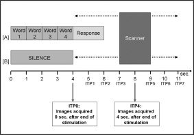
Experimental stimulation (A). Experimental condition (B). Control condition as well as image acquisition for STsamp. The delay between the end of the auditory stimulation and the beginning of the image acquisition was varied over 8 s. Each ITP corresponds to the volume acquired after the end of auditory stimulation, e.g., ITP0 corresponds to volumes acquired 0 s after the end of the auditory stimulation, and ITP5 corresponds to volumes acquired 5 s after the end of the auditory stimulation.

Overall, 41 concrete one‐syllable words spoken by a female voice were presented in four‐word sequences. The recorded words had an average concreteness factor of 463 (range: 234–614) and an average frequency factor of 56 (range: 1–362) based on the MRC Psycholinguistics Database (Machine Usable Dictionary, v. 2.0). All words were recorded using Audacity (http://audacity.sourceforge.net/) and were normalized for their root‐mean‐square energy. The number of four‐word sequences (n = 48) did not differ between the STsamp and the ERcont design (see below). During the BIG‐CVA design, 106 four‐word sequences were presented. The ERcont and the STsamp conditions had a minimum 4 s nonstimulus gap between auditory stimulations, whereas the BIG‐CVA sequence had a minimum nonstimulus gap of 2 s (the duration of the SBN) if two experimental trials followed each other. The frequency of hit targets was 50% for all designs. Behavioral correlates were obtained in percent correct and nonparametric tests were used to assess possible interdesign differences. The three acquisition types are described below. The order in which the three scans were performed was randomized across subjects.

Sparse temporal sampling design (STsamp)

Subjects listened to 48 sets of words and 16 silent periods with the same duration over the entire scanning time. Although the TR was kept constant at 16 s (flip angle 90°), the start of the 2‐s clustered MR acquisition varied with regard to the onset of auditory stimulation by pseudorandomly jittering the start of the auditory stimulation frame (4 s of words or silence) within the 16‐s TR period in 1‐s steps (see Fig. 2A). This jittering process [for details, see Gaab et al., 2003] resulted in eight image time points (ITPs). ITP0 corresponds to the scans acquired beginning 0 s after the end of the auditory stimulation, whereas ITP5 corresponds to the images acquired beginning 5 s after the end of the auditory stimulation. Overall, 66 time frames were acquired over the duration of 17 min and 34 s. In this case, both the control and experimental condition occurred during periods of scanner inactivity, and the previously determined quiescent scanner volume setting was used for stimulus presentation.

Figure 2.

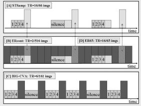
Experimental designs with timing of auditory stimulation and image acquisition. A: Sparse temporal sampling (STsamp) design. B: Event‐related with continuous scanning design (ERcont). C: Clustered volume acquisition design (BIG‐CVA). Lighter gray blocks reflect auditory/silence stimulation and darker gray (or yellow) blocks image acquisitions. D: ER65: Selecting the (in comparison to STsamp) time corresponding 65 scans (in gray/black‐yellow stripes) out of the ERcont design enables the direct comparison between the two designs and the direct assessment of the influence of SBN on signal intensities.

Event‐related continuous scanning design (ERcont)

For this condition the auditory stimulation design of the STsamp task was used but continuous scanner noise was present during the entire experiment. This method is the way in which most event‐related fMRI experiments are performed (Fig. 2B). A TR of 2 s was used for this condition with flip angle 75°, which resulted in continuous scanner noise over the entire 17 min and 12 s. Overall, 516 time frames were acquired in this condition. For these scans the volume level obtained during setup while the scanner was operating was used for presentation.

Clustered volume acquisition design (BIG‐CVA)

Subjects listened to 106 sets of words during a 2‐s clustered acquisition scan following each of the auditory stimulations (Fig. 2C). The silent condition (4 s of silence, 53 sets altogether) was pseudorandomly interleaved with the auditory condition. During this experimental condition 161 images were acquired over 16 min and 6 s. A clustered acquisition was obtained every 6 s during a 2‐s period using a flip angle of 90°. Image acquisition always started immediately after the end of auditory stimulation and no scanner noise was present during the auditory stimulation or control (no stimulus) periods. The quiescent scanner volume setting was used for stimulus presentation.

fMRI Data Analysis

fMRI data preprocessing

After image reconstruction, each set of axial images was slice time‐corrected, realigned to the first image, and coregistered with the corresponding T1‐weighted high‐resolution dataset. Spatial normalization was done in three steps. First, the skull of the T1‐weighted high‐resolution dataset was stripped using FSL (see http://www.fmrib.ox.ac.uk/fsl/). After that, all T1 images were corrected using the SPM2 bias correction and then spatially normalized to the skull‐stripped SPM2 template (Montreal Neurological Institute (MNI) space). Normalization parameters were applied to the functional images and then functional images were smoothed with an isotropic Gaussian kernel (4 mm full‐width at half‐maximum, FWHM).

Statistical analysis of group fMRI data

Statistical analysis was performed using parametric mapping software (SPM2, Wellcome Department of Cognitive Neurology, London, UK). The main data analysis was performed using a General Linear Model as implemented in SPM2 [Friston et al., 1995].

Main effects within each experimental design.

By convolving the three different task designs (using boxcars depicting each 4‐s auditory stimulus event) with a hemodynamic response function [Glover, 1999], three different covariates (BIG‐CVAcov, ERcontcov, STsampcov) were developed and entered as a regressor in three separate basic model simple regression analyses. This regressor approach was chosen to guarantee a fair comparison between the three designs. The contrast images so obtained for each subject were then entered into three separate one‐sample t‐test second‐level group analyses (one for each experimental design). All results for the random‐effects models were corrected for multiple comparisons [FDR; Benjamini and Hochberg, 1995] (P < 0.025; cluster size: 25 voxels). No direct statistical comparison was performed between the designs (see ROI analysis, below, for comparisons).

Assessing the direct influence of SBN using time corresponding images.

In order to further assess the influence of the scanner noise on intensity of auditory activations, we selected 65 evenly spaced images out of the 516 images of the ERcont condition and convolved them with STsamp covariate (here referred to as ER65). The selected scans corresponded in time with the first 65 of the 66 images for the STsamp condition, i.e., every 16 s (Fig. 2D). Because the stimulus design and statistical power of the ER65 and the STsamp condition was identical, we could directly access the influence of the scanner noise on auditory areas using this ER65 design. The contrast images were then also entered in a group analysis (one‐sample t‐test). In order to compare the STsamp and the ER65 design, we performed a paired t‐test with the contrast images. The results are presented for a threshold of P < 0.05, corrected for multiple comparisons.

Time course analysis for STsamp and ER65.

Because the gap between the end of the auditory stimulation and the start of the image acquisition for STsamp (and ER65, respectively) was varied over 8 s, we were able to perform a time course analysis even though only one set of images was acquired every 17 s. This analysis enabled us to directly compare the two designs over 8 s (eight imaging time points) following the end of the auditory stimulation to reveal possible time course differences of the HRF response in auditory as well as extratemporal areas. For the BIG‐CVA design, no time course analysis could be performed due to the fixed interval between auditory stimulation and image acquisition. In a fixed‐effects group analysis, each of the eight ITPs for each subject was modeled as a separate condition and a finite impulse response (FIR) basic set (order/window length = 1) as well as a high‐pass filter (128 s) was applied. Contrast images were created for each ITP as well as four ITP clusters (Cluster1: ITP0‐1; Cluster2: ITP2‐3; Cluster3: ITP4‐5; Cluster 4: ITP6‐7). All results in the time course analysis are corrected for multiple comparisons (P < 0.05; family‐wise error (FWE) corrected, cluster size = 25).

Movement parameter analysis

In order to compare design‐related movement for each possible movement direction (x, y, z, pitch roll yaw; absolute movement from first image), we created a mean movement value for each direction and each subject. The six movement parameters were then compared between the three experimental conditions using Friedman and Wilcoxon tests.

ROI Delineation

Four anatomically defined ROIs were chosen for this analysis using the software program WFU_pick Atlas and the implemented AAL atlas [Maldjian et al., 2003, 2004; Tzourio‐Mazoyer et al., 2002]. We chose separately for the right and left hemisphere the following predefined ROIs: 1) the transverse gyrus (Heschl's gyrus) covering primary auditory cortex, and 2) the superior temporal gyrus covering higher‐order auditory regions. Four individual t‐maps were created for each subject (BIG‐CVA, ERcont, STsamp, ER65) using a single regression analysis (basic models) with the corresponding covariates (see above). For the ITP analysis, a t‐map for each ITP (see detailed analysis description above) and each subject within the fixed‐effects model was created for ER65 and STsamp. For this analysis, standard errors were obtained from each subject's t‐map (see below).

ROIs were applied to the t‐map images for each subject separately and region‐specific values were averaged over all subjects for each of the three designs as well as the subset ER65. Then nonparametric statistical tests (Friedman and Wilcoxon tests) were applied in order to assess possible statistical differences between experimental designs or hemispheres.

Comparison with Theory

In any task design there is an inverse relationship between the average interstimulus interval (ISI) and the number of time frames that can be acquired at constant total scan time. For a long ISI, such as in STsamp, fewer frames are acquired with concomitantly reduced degrees of freedom (df) in the fixed effects modeling, with the opposite true for continuous scanning. However, with longer average ISI the hemodynamic response recovers more fully to baseline condition, which provides a larger signal that in turn can offset the reduced df.

We calculated the expected BOLD contrast‐to‐noise ratio (CNR) for each of the four designs, based only on the hemodynamic response to the auditory task and ignoring the influence of the SBN, i.e., nonlinearities due to masking or other neuronal effects, but taking into account baseline shifts that might result from nonreturn to equilibrium of the HRF as well as T1 relaxation effects that varied with the repetition time, TR. We hypothesized that if masking occurred the measured data would have lower relative signal intensities than that calculated with neural effects ignored. Using the covariate vectors C(n) obtained from the experimental design (Fig. 2) convolved with a hemodynamic response function [Glover, 1999], the BOLD contrast B is proportional to the root mean square average of the power in the covariate [Papoulis, 1977]:

(1)

where N is the number of time frames in the design, the overbar denotes average over the time series, and Ψ is the NMR relaxation factor [Haacke, 1999] applicable when the Ernst flip angle is used:

(2)

The Ernst angle may not be optimal when inflow effects are present [Lu and Golay, 2002]. Then the CNR is proportional to B√df, so that:

(3)

Using Eq. 3 and a T1 of 1350 ms for gray matter, values of CNR were computed for the BIG‐CVA, STsamp, ERcont, and ER65 designs using T1 = 900 ms and df = {139, 64, 256, 63}, respectively (accounting for autocorrelation due to the HRF). We compared these calculated values with measured t‐scores (analogous to CNR) obtained from the ROIs above as a grand average over all subjects and left and right Heschl's gyri and left and right STG. Since the amplitude of the CNR in Eq. 3 has an implicit arbitrary constant multiplier, the calculations were normalized to the measured STsamp t‐scores to examine relative values.

RESULTS

Behavioral Results

All subjects performed above 83% correct for all three conditions. The mean performance for ERcont was 96% correct, for STsamp it was 99% correct, and for BIG‐CVA it was 92% correct. A Friedman test showed significant differences between the three experimental conditions (χ² = 11.7, P = 0.003). Post‐hoc Wilcoxon tests revealed superior performance for the STsamp vs. ERcont condition (Z = −2.5, P = 0.01) and for the STsamp vs. BIG‐CVA condition (Z = −2.6, P = 0.009).

Movement Parameter Analysis

Only analysis for the y‐direction showed significant differences among the three experimental designs using a Friedman test (χ² = 8.6; P < 0.05). A post‐hoc analysis (Wilcoxon tests) showed less movement in the y‐direction in the BIG‐CVA (mean: 0.27 mm) vs. the ERcont (mean: 0.50 mm) condition (Z = 1.98; P < 0.05). Since even the most significant difference was subvoxel and image coregistration was used during all preprocessing, further statistics are not reported.

Auditory Setup Results

Subjects chose on average an SPL amplitude of 61.6 (±4.8) dB (A) for STsamp and BIG‐CVA, and 72.8 (±6.0) dB (A) for ERcont. The SPL for the scanner background noise was measured as 116 dB (A). The isolation of the headphone was not measured but was estimated to be ∼35 dB.

Imaging Results

The random‐effects analyses were corrected for multiple comparisons using the false discovery rate [e.g., Genovese et al., 2002]. We used a threshold of P < 0.05 for the direct comparison between STsamp and the subset ER65. For the group analyses assessing the main effect within each experimental design we used a more stringent threshold (P < 0.025) because the P < 0.05 threshold led to large clusters that extended so much that it was difficult to discern auditory regions.

The fixed‐effects analysis assessing the Cluster ITP analysis was corrected for multiple comparisons using the family‐wise error rate [e.g., Nichols and Hayasaka, 2003].

Group analysis

Main effect within each experimental design (Fig. 3, Table I).

Figure 3.

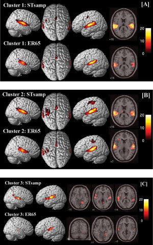
Imaging results for the three experimental designs and the subset ER65 (P < 0.025, corrected for multiple comparisons, false discovery rate (FDR)). Each row depicts one of the four designs in 3D rendering (left 2 columns) and in axial slices (right 3 columns) for activations in Table I. [Color figure can be viewed in the online issue, which is available at www.interscience.wiley.com.]

Table I.

Activation table for the three experimental designs and the subset ER65

Region	Extent	MNI coordinates			T
		x	y	z
CVA
Left superior temporal gyrus	865	−58	8	−2	15.50
Cingulate gyrus	66	−8	4	50	10.07
Right superior temporal gyrus	744	56	−28	16	12.89
Left caudate nucleus	73	−22	8	16	12.34
Right caudate nucleus	26	18	−2	16	9.03
Right dorsal cerebellum	41	20	−58	−22	10.01
Right dorsal cerebellum	64	18	−68	−24	8.62
Stsamp
Left superior temporal gyrus	781	−60	−26	12	10.61
Right superior temporal gyrus	663	58	−30	16	9.07
Cingulate gyrus	294	−2	2	42	8.45
Left caudate nucleus	223	−24	8	14	7.75
Right caudate nucleus	176	24	−24	14	7.39
Left inferior frontal gyrus	98	−36	26	8	7.20
Right dorsal cerebellum	113	20	−68	−18	7.13
Left postcentral gyrus/inferior parietal area	136	−48	−32	52	7.06
Thalamus (medial dorsal nucleus)	30	−10	−22	10	6.10
ER65
Right superior temporal gyrus	241	62	−26	12	17.17
Left superior temporal gyrus	56	−51	−22	6	11.07
Ercont
Cingulate gyrus	81	10	16	36	16.62
Cingulate gyrus	362	2	2	46	7.73
Right superior temporal gyrus	782	66	−10	4	14.32
Left superior temporal gyrus	794	−54	−20	12	12.50
Left postcentral gyrus/inferior parietal area	235	−46	−34	46	11.66
Right inferior frontal gyrus	32	38	28	8	8.86
Left insula	28	−38	14	14	8.07
Left caudate nucleus	65	−18	8	8	7.32
Thalamus (medial dorsal nucleus)	92	−11	−16	12	6.91
Left inferior frontal gyrus	42	−34	28	6	6.86

All results are reported for P < 0.025, corrected for multiple comparisons.

ER, event‐related; MNI, Montreal Neurological Institute; CVA, clustered volume acquisition; Stsamp, sparse temporal sampling.

All three designs yielded bilateral activations of superior temporal gyri including Heschl's gyrus and the planum temporale, the anterior cingulate, and the left caudate nucleus. The two silent designs (BIG‐CVA and STsamp) also yielded activation in the right dorsal cerebellum. Only the BIG‐CVA design led to activation of the right caudate nucleus. Additional results for the STsamp and ERcont include the left postcentral gyrus/inferior parietal region, the left inferior frontal gyrus, and the thalamus. The ERcont design also revealed activations of the right inferior frontal gyrus and the left insula.

Because of design limitations the BIG‐CVA scan duration was 93% as long as that for the ERcont and STsamp designs. This reduced the statistical power of the BIG‐CVA activation a small amount. However, we verified that no essential difference was observed in the activation comparisons for two subjects when the scan durations were equalized by removing data from the ERcont and STsamp scans.

Assessing the direct influence of SBN using time corresponding images.

The ER65 design led to activations of bilateral superior temporal gyrus, including Heschl's gyrus and the planum temporale (Fig. 3, Table I). Direct comparisons showed that STsamp yielded greater activation than ER65 in bilateral superior temporal gyrus and a network of extratemporal brain regions including bilateral supramarginal gyrus, right pre‐SMA, bilateral inferior temporal gyrus, and temporoparietal regions (Fig. 4).

Figure 4.

Imaging results (random‐effects analysis) for the direct comparison between STsamp and ER65 (P < 0.05, corrected for multiple comparisons, FDR). [Color figure can be viewed in the online issue, which is available at www.interscience.wiley.com.]

ROI analysis

Hemispheric ROI differences.

There were significant higher mean t‐values in left than right superior temporal gyrus for all designs except for ERcont (Fig. 5B, Table III). There were no significant hemispheric differences in Heschl's gyrus (Fig. 5A, Table III).

Figure 5.

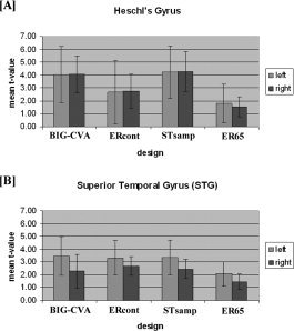
Results for the ROI analysis for the three experimental designs and the subset ER65: (A) Heschl's gyrus (B) superior temporal gyrus.

Table III.

ROI analysis for hemispheric differences

ROI	Design	Hemispheric asymmetry	Z value	P value
Heschl's gyrus
	BIG‐CVA	Left = Right	−0.153	P = 0.878
	STsamp	Left = Right	−0.474	P = 0.635
	ERcont	Left = Right	−0.459	P = 0.646
	ER65	Left = Right	−0.357	P = 0.721
Superior temporal gyrus
	BIG‐CVA	Left > Right	−2.80	P < 0.01*
	STsamp	Left > Right	−2.39	P < 0.05*
	ERcont	Left = Right	−1.83	P = 0.06
	ER65	Left > Right	−2.09	P < 0.05*

ROI, region of interest; ER, event‐related; BIG‐CVA, behavior interleaved gradient, clustered volume acquisition; Stsamp, sparse temporal sampling.

Interdesign ROI differences (Fig. 5, Table IV).

Table IV.

Interdesign ROI analysis

ROI	Statistical test	Designs tested	Hemisphere	Design differences	Z value/chi2 value	P value
Heschl's gyrus
	Friedman	All	Left	Yes	Chi2 = 18.36	P < 0.00
		All	Right	Yes	Chi2 = 16.56	P < 0.01
	Wilcoxon	BIG‐CVA/STsamp	Left	No	Z = −0.255	P < 0.79
		BIG‐CVA/STsamp	Right	No	Z = −0.051	P < 0.95
		BIG‐CVA/ERcont	Left	BIG‐CVA > ERcont	Z = −2.09	P < 0.05
		BIG‐CVA/ERcont	Right	No	Z = −1.58	P < 0.11
		BIG‐CVA/ER65	Left	BIG‐CVA > ER65	Z = −2.29	P < 0.05
		BIG‐CVA/ER65	Right	BIG‐CVA > ER65	Z = −2.59	P < 0.01
		STsamp/ERcont	Left	STsamp > ERcont	Z = −2.59	P < 0.01
		STsamp/ERcont	Right	STsamp > ERcont	Z = −2.29	P < 0.05
		STsamp/ER65	Left	STsamp > ER65	Z = −2.80	P < 0.01
		STsamp/ER65	Right	STsamp > ER65	Z = −2.80	P < 0.01
		ERcont/ER65	Left	ERcont > ER65	Z = −2.19	P < 0.05
		ERcont/ER65	Right	ERcont > ER65	Z = −2.49	P < 0.05
Superior temporal gyrus
	Friedman	All	Left	Yes	Chi2 = 11.64	P < 0.01
		All	Right	Yes	Chi2 = 13.44	P < 0.01
	Wilcoxon	BIG‐CVA/STsamp	Left	No	Z = −0.561	P = 0.57
		BIG‐CVA/STsamp	Right	No	Z = −0.878	P = 0.87
		BIG‐CVA/ERcont	Left	No	Z = −0.408	P = 0.68
		BIG‐CVA/ERcont	Right	No	Z = −0.968	P = 0.33
		BIG‐CVA/ER65	Left	No	Z = −1.784	P = 0.74
		BIG‐CVA/ER65	Right	No	Z = −1.682	P = 0.93
		STsamp/ERcont	Left	No	Z = −0.255	P = 0.79
		STsamp/ERcont	Right	No	Z = −0.663	P = 0.50
		STsamp/ER65	Left	STsamp > ER65	Z = −2.65	P < 0.01
		STsamp/ER65	Right	STsamp > ER65	Z = −2.80	P < 0.01
		ERcont/ER65	Left	ERcont > ER65	Z = −2.80	P < 0.01
		ERcont/ER65	Right	ERcont > ER65	Z = −2.49	P < 0.05

ROI, region of interest; ER, event‐related; BIG‐CVA, behavior interleaved gradient, clustered volume acquisition; Stsamp, sparse temporal sampling.

For the ROIs in Heschl's gyrus there were significant increases in the mean t‐values for BIG‐CVA in comparison to ERcont in the left hemisphere and to ER65 bilaterally. There were no significant differences when comparing BIG‐CVA to STsamp (P < 0.79 for left and P < 0.95 for right hemisphere). STsamp showed significantly higher t‐values than ERcont and ER65 bilaterally (Fig. 5A, Table IV).

The analysis of the ROI covering the superior temporal gyrus revealed increased mean t‐values for the left and right hemisphere for ERcont and STsamp in comparison to the ER65 bilaterally. No differences were found between ERcont, BIG‐CVA, and STsamp, although similar trends to those observed for Heschl's gyrus were demonstrated (see Fig. 5B, Table IV).

Imaging time point (ITP) analysis for STsamp and ER65.

ROI results.

Results yielded for all four ROIs and ITP0‐5 higher mean t‐values for STsamp than ER65. Besides the overall mean t‐value differences, the time courses and peak ITP within each ROI differ between the two designs (see Fig. 6A–D).

Figure 6.

Results for the ROI time point analysis for STsamp and ER65 for (A) left Heschl's gyrus (B) right Heschl's gyrus (C) left superior temporal gyrus (D) right superior temporal gyrus.

ITP imaging results.

Results for cluster 1 revealed activation of superior temporal gyrus and the cingulate gyrus for both designs and additional activation of the left precentral gyrus for STsamp in comparison to ER65 (cluster 1: ITP0‐1; Fig. 7A, Table II).

Figure 7.

Imaging results for the cluster analysis for STsamp and ER65 (P < 0.05, corrected for multiple comparisons (FWE)) (A) cluster 1 (ITP0‐1), (B) cluster 2 (ITP2‐3), (C) cluster 3 (ITP4‐5). Cluster 4 did not reveal significant voxels for this threshold. 3D‐rendered images (left) and axial slices (right) are selected based on regions activated in experimental designs as shown in Table II. [Color figure can be viewed in the online issue, which is available at www.interscience.wiley.com.]

Table II.

Activation table for cluster 1–3 for STsamp and ER65

Region	Extent	MNI coordinates			T
		x	y	z
STsamp:
ITP0–1
Left superior temporal gyrus	2787	−56	−14	8	24.78
Right superior temporal gyrus	2339	58	−10	8	20.07
Cingulate gyrus	188	−4	6	46	9.03
Left precentral gyrus	60	−50	−8	48	7.8
ITP2−3
Left superior temporal gyrus	2554	−56	−14	8	20.72
Right superior temporal gyrus	1949	64	−18	8	20.56
Cingulate gyrus	474	−6	16	40	11.78
Pre/postcentral gyrus	474	−42	−24	52	7.87
Left thalamus	36	−12	−18	14	6.95
ITP4–5
Right superior temporal gyrus	671	64	−18	8	13.63
Left superior temporal gyrus	1192	−64	−14	6	12.99
Right parahippocampal gyrus	418	18	−56	−10	8.36
Right supramarginal gyrus	64	62	−48	26	7.17
Left thalamus	36	−12	−16	14	6.75
Left insula	28	−40	−16	4	6.16
ITP6−7
No regions
ER65
ITP0−1
Left superior temporal gyrus	1539	−56	−12	10	15.98
Right superior temporal gyrus	1071	58	−8	8	11.25
Cingulate gyrus	200	−4	12	40	9.55
ITP2−3
Left superior temporal gyrus	1756	−60	−8	6	15.41
Right superior temporal gyrus	1292	58	−18	6	12.81
Cingulate gyrus	397	−4	18	38	9.77
Cingulate gyrus	32	6	32	30	5.85
Left inferior frontal gyrus	69	−32	24	10	9.24
Postcentral gyrus	80	−40	−24	60	7.11
Postcentral gyrus	78	−54	−26	50	6.92
ITP4−5
Left superior temporal gyrus	263	−64	−12	10	6.99
Right superior temporal gyrus	63	64	−16	4	6.99
Right parahippocampal gyrus	53	26	−44	−12	5.90
Right fusiform gyrus	34	26	−62	−10	5.89
ITP6−7
No regions

All results are reported for P < 0.05, corrected for multiple comparisons.

ER, event‐related; MNI, Montreal Neurological Institute; ITP, imaging time point; Stsamp, sparse temporal sampling.

Results for the second cluster revealed activation of bilateral superior temporal gyrus, the left postcentral gyrus, and the cingulate gyrus for both designs. Results for STsamp additionally yielded activation of left thalamus and left precentral gyrus. The analysis for ER65 revealed additional activation for left inferior frontal regions (cluster 2: ITP2‐3, Fig. 7B, Table II).

Results for the third cluster revealed activation of bilateral superior temporal gyrus and right parahippocampal gyrus. The results for STsamp revealed additional activations of right supramarginal gyrus, left insula, and left thalamus, whereas the results for ER65 additionally included the right fusiform gyrus (cluster 3: ITP4‐5, Fig. 7C, Table II). No activations were found for the last cluster for this threshold.

Comparison with theory

Figure 8 shows the averaged t‐scores for activation in auditory areas compared with CNR values calculated according to Eq. 1, normalized with STsamp. The calculations predict higher CNR for both BIG‐CVA and ERcont and greatly decreased CNR for ER65 relative to STsamp, primarily as a consequence of the number of independent samples in each, but also modulated by hemodynamic recovery differences. However, the measured t‐scores for BIG‐CVA are comparable to STsamp and considerably lower than predicted. Furthermore, the measured t‐scores for ERcont are 60% of that calculated and substantially less than STsamp even though approximately 8 times as many time frames are collected with the continuous design. Finally, the measured values for ER65 are significantly lower than those measured for STsamp in all ROIs (see ROI analysis, above), directly demonstrating the deleterious effects of masking by the SBN, since the two designs have exactly the same auditory stimulation and number of time frames (statistical power) but differ only by the amount of scanner background noise. We verified that the calculation of signal in Eq. 2 using the Ernst angle was reasonable by measuring the SNR in Heschl's gyrus for one subject in both ERcont and STsamp and found a ratio of 0.69, close to the 78% expected. In fact, if this measured value is used instead of the assumed calculation, the discrepancy in Figure 8 between ERcont predicted/measured and STsamp becomes even larger, further confirming the source of disparity as due to SBN.

Figure 8.

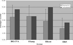
Comparison of activation measured in auditory ROIs with CNR calculated for each design, based on response to auditory stimuli normalized to the STsamp design. ER65 shows much lower values than predicted and significantly lower values (see ROI Analysis) than STsamp due to masking and elevated baseline effects.

DISCUSSION

This study examined the influence of three different experimental designs with varying degrees of scanner background noise (SBN) on the functional anatomy, signal intensities, and time courses of activations in auditory and extratemporal areas. Behavioral performance was higher in the STsamp condition, indicating that the potentially deleterious effects of long intertrial intervals on performance was more than compensated for by the SBN‐free presentation of the auditory material. The BIG‐CVA design also presented auditory stimuli without SBN, but the increased number of trials, the decreased time gap between trials, and suboptimal TR may have had led to decreased performance scores. Concordantly, all three designs (BIG‐CVA, ERcont, STsamp) showed activation in a functional network that included superior temporal areas, anterior cingulate, and caudate nucleus. Within the temporal lobe, activation was equal bilaterally in primary auditory cortex (Heschl's gyrus), but left‐lateralized in secondary auditory cortex of the superior temporal gyrus. This is consistent with the view that hemispheric specialization is not apparent in early or primary cortical processing, but lateralized (in this case left‐lateralized for verbal material) in later or secondary cortical processing [e.g., Binder et al., 1997, 2000; Giraud and Price, 2001; Poeppel et al., 2004]. Nevertheless, the mean t‐values within auditory and extratemporal areas varied among the three designs, suggesting SBN‐induced masking effects of the BOLD response, especially within Heschl's gyrus, for the designs with continuous SBN.

Heschl's Gyrus and SBN

In agreement with several previous studies that reported a negative influence of SBN on signal intensities within primary auditory regions, our ROI results suggest SBN‐induced masking of the auditory cortical response within Heschl's gyrus as a result of increased SBN (ERcont and ER65). This is further supported by our comparison between the theoretical prediction of the signal intensity and the actual measured values. The design with continuous SBN, ERcont, resulted in decreased values for measured compared to predicted signal intensities, which further suggests SBN‐induced masking of the BOLD response. However, several other factors might have influenced this comparison, such as attentional demands during the experiment, differences in the time course of the HRF for the designs, or delayed activation within some regions.

The present study showed no significant differences between the BIG‐CVA and the STsamp design for both ROIs covering Heschl's gyrus, despite the greater number of acquired images as well as the quantity of word sequences presented for the BIG‐CVA design (106 experimental and 55 control for BIG‐CVA vs. 48 experimental and 16 control for STsamp). This suggests that the signal gains from STsamp measurement makes up for the 50% reduction of observations. The signal gain in the STsamp design despite the reduced number of observations suggests SBN‐induced masking effects of the BOLD response in the BIG‐CVA design. This might be due to the lack of jittering and/or the TR of 6 s, which does not allow the SBN‐induced activation to recover before the next acquisition. Based on the literature on the shape of the HRF following an auditory stimuli [Glover et al., 1999] or SBN in particular [Hall et al., 2000], the SBN‐induced HRF should peak around 4–6 s after the auditory stimulus. During a BIG‐CVA design with a TR of 6 s, the HRF induced by image acquisition (SBN) #X would peak during image acquisition (SBN) #X+1.

Furthermore, the measured t‐scores for BIG‐CVA are considerably lower than predicted. This is consistent with the explanation that the signal is reduced with the nonjittered design of BIG‐CVA because the HRF peaks after the scan and is thus not sampled at its largest, and is reduced further by SBN‐induced masking of the BOLD response and elevated baseline from the remnant HRF of the previous scan's SBN. Nevertheless, one other potential source of difference between the two designs might be the nature of the tasks. The BIG‐CVA design uses a TR of 6 s, which leads to continuous auditory stimulation as well as a minimum nonstimulus gap of 2 s if experimental trials follow each other (in comparison to 4 s or greater for the other designs). A BIG‐CVA design with a longer TR might have reduced the HRF effects due to the SBN and at the same time increased the gap between stimulations, but then a sparse temporal sampling design with a jittered delay (and time course information) seems to be the more appropriate design.

By extracting a subset of images taken out of ERcont (ER65) and comparing directly to STsamp, we are able to assess the influence of SBN while keeping the experimental auditory stimulation as well as the quantity of observations constant. One difference between these two designs was an increased amplitude of the auditory stimulation for the ER65 design. However, since previous studies have shown increased activation and spatial extent with increased stimulus amplitude [Jancke et al., 1998; Lasota et al., 2003], this might have led to a slight advantage for the ER65 design.

The comparison showed greater mean t‐values for STsamp in Heschl's gyrus and STG in both hemispheres, which indicates strong SBN‐induced masking of the BOLD response. Nevertheless, it remains unclear whether this “masking” is a result of the nonlinearity of the human auditory cortex or an effect of raised signal intensities within the control baseline condition [see Talavage and Edmister, 2004]. Further experiments are necessary in order to answer this question [see Gaab et al., 2006].

Extratemporal Regions and SBN

Most previous studies examined only primary auditory areas, but the influence of SBN might also be reflected in nonauditory, extratemporal areas. BIG‐CVA, STsamp, and ERcont revealed additional activation of nonauditory areas, including the anterior part of the cingulate gyrus. This area has been known to be involved in attention generally [e.g., Loose et al., 2003] and auditory selective attention particularly [Sevostianov et al., 2002]. Since all three experimental designs showed activation of the anterior cingulate, an SBN‐induced task difference or attention modulation within this area between ERcont and the “silent” designs seems unlikely. Nevertheless, we contrasted the word sequence task with a no‐stimulus condition, which is usually not the case in fMRI studies. The question whether SBN may influence attentional demands in experimental and control conditions differently cannot be answered from our study and further studies should address this issue. Additionally, all three designs revealed activation of the caudate nucleus. Several studies have demonstrated caudate activations in working memory tasks [Lewis et al., 2004; Owen et al., 1996; Postle and D'Esposito 1999a, b; Speck et al., 2003]. Some of these studies suggested that the caudate nuclei may be more involved in spatial than nonspatial working memory, suggesting a role in the integration of spatially coded mnemonic information with motor preparation to guide behavior. However, Lewis et al. [2004] demonstrated activation of the caudate nucleus in a nonspatial working memory task and the critical role of the caudate nuclei in cognitive processes has also been underlined by neurodegenerative conditions such as Huntington's disease.

Furthermore, the two silent designs (BIG‐CVA and STsamp) showed additional activation of the right dorsal cerebellum [Area V+VI; Schmahmann et al., 1999] which was not present in the ERcont condition for the given threshold. Several studies have emphasized the role of the cerebellum in auditory processing [e.g., Gaab et al., 2003; Holocomb et al., 1998; Jancke et al., 2000; Mathiak et al., 2004; Silveri et al., 1998], auditory verbal memory function [e.g., Andreasen et al., 1995; Desmond et al., 1997; Grasby et al., 1993; Kirschen et al., 1995; Schumacher et al., 1996], as well speech perception or silent speech [Ackermann et al., 2004; Mathiak et al., 2002; Silveri et al., 1998]. The fact that the right dorsal cerebellum is only activated in the silent designs at this threshold and not in ERcont leads to the assumption that the SBN‐induced masking of the BOLD response within ERcont might have also affected cerebellar activations. The SBN contaminated baseline might already have led to cerebellar activations and therefore the signal intensity of the cerebellum during the word task might not differ significantly from the baseline condition. Adding words to the SBN (experimental condition) might not enhance the signal to a degree that a direct comparison (Words + SBN > SBN) leads to significant increased activation within the cerebellum.

The STsamp and ERcont design showed additional activation of the left inferior frontal gyrus, the thalamus (medial dorsal nucleus), and left postcentral gyrus/inferior parietal region. None of these areas were observed during the BIG‐CVA condition. Similar network components were previously reported by several studies examining auditory and verbal working memory [e.g., Derrfuss et al., 2004; Grasby et al., 1994; LaBar et al., 1999]. The lack of activation at the given threshold within these areas in the BIG‐CVA design might be due to the deficient sampling of the HRF response. The BIG‐CVA design is not jittered and occurs always 2 s after the end of the auditory stimulation. We assume that only a narrow part of the HRF will be picked up by this one scan and that the above‐mentioned regions might show different time courses. Furthermore, the nature of the task is different in the BIG‐CVA design since it only allows very short gaps between the button response and the start of a new trial. Trial‐to‐trial interference may have altered attentional demands between the designs.

The ERcont design revealed activation of right inferior frontal gyrus and left insula. It remains unclear why the ERcont design shows additional activation of these areas at the given threshold. On the one hand, one could argue that right inferior frontal and left insula regions are part of the functional network of verbal working memory and that increased quantity of observations and therefore increased statistical power are necessary in order to reach statistical significance in these regions. On the other hand, these areas could be involved in the inhibition of the SBN during ERcont or in allocating auditory attention. Vorobyev et al. [2004] found activation of left insula during the selective processing of text and speech and Muller et al. [2003] reported insula activation in response to target detection in an auditory oddball task.

STsamp, ER65, and Time Course Information

The ITP analysis revealed robust t‐scores despite a modest number of samples per time point. This is an advantage of any jittered design [Liu and Frank, 2004]. An advantage of the STsamp design in comparison to BIG‐CVA is the jittering of the delay between the end of the auditory stimulation and the beginning of the image acquisition. This enables the examination of the activation time course over a period of time, here over 8 s (ITP0–ITP7). In order to assess SBN‐induced time course differences, we further examined the time course for STsamp and the subset ER65. Comparing all ITPs together revealed activation of the superior temporal gyri during STsamp compared to ER65, which is most likely the result of SBN‐induced masking of the BOLD response during ER65.

The clustered ITP analysis revealed time course differences between STsamp and ER65. Cluster 1 (ITP0‐1) demonstrated similar regions for STsamp and ER65, although the precentral gyrus was activated during STsamp at the given threshold. This is most probably due to the required button‐press response, and cluster 2 shows activation of precentral/postcentral areas for both designs. The second cluster also revealed a similar activation pattern between the two designs but STsamp showed additional activation of a left thalamic region, whereas ER65 activated an inferior frontal region. The overall ITP analysis (see above) also revealed left thalamic activation in ERcont and the lack of activation in ER65 in this region might be due to statistical power. The third cluster shows a series of brain regions for ER65 and STsamp that were not present during the overall analysis (all ITPs), such as the parahippocampal, supramarginal, or fusiform gyrus. Nevertheless, these areas were previously shown to be involved in verbal tasks as well as auditory or verbal working memory tasks [e.g., Binder et al., 1997; Gaab et al., 2003; Sakai et al., 2004]. The lack of significant activation in cluster 4 (ITP6‐7) indicates that activation rapidly decayed after ITP5.

The differences of the neural networks between clusters 1 and 3 in both designs shows the advantage of assessing ITPs or ITP clusters separately, which may demonstrate not only differences in signal intensities in key regions but also to changes in the functional network during the time course of task processing.

Implications for Assessing Auditory Processing in the MR Environment

Our present study examined designs with overall durations around 17 min but various TRs. One possible confound in using longer TRs is the general presumption that longer TRs and therefore longer “waiting times” between the experimental trials might lead to increased head movement within the MRI scanner. However, our analysis demonstrated a small contrary effect, namely, head movement was greater during the continuous scan (ERcont) in comparison to the BIG‐CVA design. Nevertheless, many experimenters seek to avoid long experimental durations and results might differ when implementing shorter runs. However, sparse temporal sampling with shorter run duration has been successfully used for examining small children (e.g., 5–7 years old) [Overy et al., 2004].

Overall, both BIG‐CVA and STsamp are powerful designs to assess auditory processing in the MR environment, especially within Heschl's gyrus, where we observed the biggest differences between the “silent” designs and the design with continuous SBN.

Nevertheless, the major difference between the BIG‐CVA design and STsamp is the sampling of the time course following the auditory stimuli. Varying the delay between the end of the auditory stimulation and the beginning of the image acquisition in STsamp enables us to sample the HRF in response to the verbal task over a period that encompasses much of the HRF (here 8 s).

In principle, the fact that images are always acquired at exactly the same time point in relation to the beginning of the auditory stimulation (4 s after beginning of first word or ITP0) is a disadvantage of the BIG‐CVA design. The sampling of the entire HRF in the ERcont design is a major advantage for this technique since interesting differences in temporal characteristics may be derived from the initial slope of the HRF curve. The additional network components in STsamp and ERcont for the given threshold might be involved later during the time course of the HRF following the auditory stimulation, and therefore not captured during a single image acquisition at a fixed time point of 4 s following the onset of the first word. Furthermore, during the BIG‐CVA design with a TR = 6, the peak as well as decay of the HRF in response to image acquisition #X will most likely be sampled during the next image acquisition #X+1 or even #X+2, which may result in SBN‐induced masking of the BOLD response within auditory and/or nonauditory areas. The nonsignificant difference within auditory areas for BIG‐CVA in comparison to STsamp could be an indicator of SBN‐induced masking of the BOLD response in the BIG‐CVA design or it could be due to the lack of time course sampling in the BIG‐CVA design.

We found no significant signal intensity differences in superior temporal gyrus among the three designs. This suggests that the influence of the SBN is much weaker in higher‐order auditory regions that should be considered when deciding on an experimental design with auditory stimulation. Depending on the experimental hypothesis, the ERcont design might have advantages over the silent designs (see also Table V with practical implications). Additional areas only observed in ERcont could be due to increased statistical power in extratemporal areas or inhibition of SBN. It remains unlikely that no additional areas are involved while listening to words and at the same time inhibiting the SBN in comparison to a baseline where only SBN is present. Listening to words with the presence of SBN seems more like a selective or divided attention task where attention to one set of stimuli (words) is required, whereas cognitive inhibition is necessary to neglect the second set (SBN).

Table V.

Proposed practical guidelines for the experimental design decision when using auditory stimuli

“Silent” designs

Suggested to use if:

• Experimental hypothesis implements interpretations of signal intensities within auditory cortex

• Subject group might have difficulties with SBN (selective attention, hearing threshold, increased task difficulty; e.g., children, elderly, patients)

• Experimental hypothesis is based on auditory selective attention, e.g., dichotic listening

• Auditory stimulus does not exceed 6 s or only parts of HRF are from interest for hypothesis

• Hypothesized functional network contains primary auditory cortex

• Multiple sessions will be scanned (e.g., pre‐post training/medication; longitudinal studies) AND attention to SBN may vary over time (e.g., improved attention/hearing; emotional state might change)

Please note: If time course of activation (HRF) should be assessed the use of a jittered “silent” method such as jittered STsamp is suggested

ERcont

Suggested to use if:

• Experimental hypothesis implements interpretations of signal intensities outside of auditory regions(extratemporal areas)

• Subjects are normal healthy adults and difficulties with SBN are not expected

• Experimental hypothesis is not based on selective attention

• Experimental design has more than two experimental conditions and/or baselines (otherwise increased session duration or decreased statistical power or decreased number of imaging time points (ITPs))

• Auditory stimulus exceeds 6 s and entire HRF is from interest for hypothesis

• Hypothesized functional network does not contain primary auditory cortex.

• Multiple sessions will be scanned (e.g., pre‐post training/medication; longitudinal studies) AND attention to SBN may not vary over time

Therefore, this “selective attention” task might lead to differences in attentional demands and might be especially difficult for children and the elderly as well as patients. Studies showing differences in the functional anatomy between healthy young adult subjects and these populations may have neglected possible differences in general and selective attention to the SBN [e.g., Konrad et al., 2005, 2006; Townsend et al., 2006]. Furthermore, the attentional demands may vary between scanning sessions (e.g., pre‐post training and remediation studies) or even within sessions.

The STsamp design seems to be effective in assessing auditory processing, and additionally enables the researcher to obtain a time course of activation. Pilot studies should be performed in order to explore the required number of ITPs to sample the entire or parts of the HRF depending on the experimental hypothesis. However, due to the long TR the development of STsamp designs that require more than two conditions seems difficult. Such studies would require extremely long sessions that would most likely be accompanied with fatigue, lack of concentration, lowered attentional effort/arousal, increased automaticity in task execution, or increased head movement. Furthermore, if the presented stimulus exceeds 6 s then using STsamp might be disadvantageous since the entire HRF cannot be sampled. However, STsamp can be used if only parts of the HRF are of interest (e.g., the decision process and not the perceptual component). Additionally, if the experimental hypothesis is not directly linked to auditory areas, then using an ERcont design might be advantageous due to increased statistical power. If the time course of activation is not of great interest for the hypothesis then BIG‐CVA might be the appropriate design for assessing auditory processing especially when more than two conditions are examined.

Furthermore, there are many other types of “silent” acquisition designs or hardware improvements that should also be considered during the experimental planning phase such as, e.g., “gradient smoothing” [Henning and Hodapp, 1993; Oesterle et al., 2001; for a review, see, e.g., Amaro et al., 2002].

Overall, the results of this study point to a multifaceted set of variables that should be considered prior to the design of an experiment that employs auditory stimulation. Important variables to take in consideration are, e.g., subject group, required attention during task, duration of the experiment, stimulus length, required time course information (e.g., number of ITPs), experimental hypothesis and hypothesized functional network, statistical power, number of conditions, number of slices acquired, as well as overall difficulty of the task. Table V summarizes our results as guidance for the experimental design decision within the auditory domain.

REFERENCES

- Ackermann H, Mathiak K, Yvry RB ( 2004): Temporal organization of “internal speech” as a basis for cerebellar modulation of cognitive functions. Behav Cog Neurosci Rev 3: 14–22. [DOI] [PubMed] [Google Scholar]
- Amaro E, Williams SCR, Shergill SS, Fu CHY, MacSweeney M, Picchioni MM, Brammer MJ, McGuire PK ( 2002): Acoustic noise and functional magnetic resonance imaging: current strategies and future prospects. J Magn Reson Imaging 16: 497–510. [DOI] [PubMed] [Google Scholar]
- Andreasen NC, O'Leary DS, Cizadlo T, Arndt S, Rezai K, Watkins GL, Ponto LL, Hichwa RD ( 1995): II. PET studies of memory: novel versus practiced free recall of word lists. Neuroimage 2: 296–305. [DOI] [PubMed] [Google Scholar]
- Bandettini PA, Jesmanowicz A, Van Kylen J, Birn RM, Hyde JS ( 1998): Functional MRI of brain activation induced by scanner acoustic noise. Magn Reson Med 39: 410–416. [DOI] [PubMed] [Google Scholar]
- Baumgart F, Gaschler‐Markefski B, Tempelmann C, Tegeler C, Heinze HJ, Scheich H ( 1996): Masking of acoustic stimuli by the gradient noise alters the fMRI detectable activation in a particular human auditory cortex. MAGMA 4: 185. [Google Scholar]
- Belin P, Zatorre RJ, Hoge R, Evans AC, Pike B ( 1999): Event‐related fMRI of the auditory cortex. Neuroimage 10: 417–429. [DOI] [PubMed] [Google Scholar]
- Benjamini Y, Hochberg Y ( 1995): Controlling the false discovery rate: a practical and powerful approach to multiple testing. J R Stat Soc Ser B 57: 289–300. [Google Scholar]
- Bilecen D, Radu EW, Scheffler K ( 1998): The MR tomography as a sound generator: fMRI tool for the investigation of the auditory cortex. Magn Reson Med 40: 934–937. [DOI] [PubMed] [Google Scholar]
- Binder JR, Frost JA, Hammeke TA, Cox RW, Rao SM, Prieto T ( 1997): Human brain language areas identified by functional resonance imaging. J Neurosci 17: 353–362. [DOI] [PMC free article] [PubMed] [Google Scholar]
- Binder JR, Frost JA, Hammeke TA, Bellgowan PSF, Springer JA, Kaufman JN, Possing ET ( 2000): Human temporal lobe activation by speech and nonspeech sounds. Cereb Cortex 10: 512–528. [DOI] [PubMed] [Google Scholar]
- Cho ZH, Park SH, Kim JH, Chung SC, Chung ST, Chung JY, Moon CW, Yi JH, Sin CH, Wong EK ( 1997): Analysis of acoustic noise in MRI. Magn Reson Med 15: 815–822. [DOI] [PubMed] [Google Scholar]
- Cho ZH, Chung SC, Lim DW, Wong EK ( 1998): Effects of the acoustic noise of the gradient system on fMRI: a study on auditory, motor, and visual cortices. Magn Reson Med 39: 331–335. [DOI] [PubMed] [Google Scholar]
- Counter SA, Olofsson A, Grahn HF, Borg E ( 1997): MRI acoustic noise: sound pressure and frequency analysis. J Magn Reson Imaging 7: 606–611. [DOI] [PubMed] [Google Scholar]
- Counter SA, Olofsson A, Borg E, Bjelke B, Haggstrom A, Grahn HF ( 2000): Analysis of magnetic resonance imaging acoustic noise generates by a 47 T experimental system. Acta Otolaryngol 120: 739–743. [DOI] [PubMed] [Google Scholar]
- Derrfuss J, Brass M, von Cramon DY ( 2004): Cognitive control in the posterior frontolateral cortex: evidence from common activations in task coordination, interference control, and working memory. Neuroimage 23: 604–612. [DOI] [PubMed] [Google Scholar]
- Desmond JE, Gabrieli JD, Wagner AD, Ginier BL, Glover GH ( 1997): Lobular patterns of cerebellar activation in verbal working‐memory and finger‐tapping tasks as revealed by functional fMRI. J Neurosci 17: 9675–9685. [DOI] [PMC free article] [PubMed] [Google Scholar]
- Di Salle F, Formisano E, Seifritz E, Linden DEJ, Scheffler K, Saulino C, Tedeschi G, Zanella FE, Pepino A, Goebel R, Marciano E ( 2001): Functional fields in human auditory cortex revealed by time‐resolved fMRI without interference of EPI noise. Neuroimage 12: 328–338. [DOI] [PubMed] [Google Scholar]
- Eden GF, Joseph JE, Brown HE, Brown CP, Zeffiro TA ( 1999): Utilizing hemodynamic delay and dispersion to detect fMRI signal change without auditory interference: the behavior interleaved gradients technique. J Magn Reson Imaging 41: 13–20. [DOI] [PubMed] [Google Scholar]
- Edmister WB, Talavage TM, Ledden PJ, Weisskopf RM ( 1999): Improved auditory cortex imaging using clustered volume acquisition. Hum Brain Mapp 7: 89–97. [DOI] [PMC free article] [PubMed] [Google Scholar]
- Elliott MR, Bowtell RW, Morris PG ( 1999): The effect of scanner sound in visual, motor, and auditory functional MRI. Magn Reson Med 41: 1230–1235. [DOI] [PubMed] [Google Scholar]
- Engelien A, Yang Y, Engelien W, Zoana J, Stern E, Silbersweig DA ( 2002): Physiological mapping of human auditory cortices with a silent event‐related fMRI technique. Neuroimage 16: 944–953. [DOI] [PubMed] [Google Scholar]
- Friston KJ, Holmes A, Worsley KJ, Poline JB, Frith CD, Frackowiak RSJ ( 1995): Statistical parametric maps in functional imaging: a general linear approach. Hum Brain Mapp 2: 189–210. [Google Scholar]
- Fu CH, Morgan K, Suckling J, Williams SC, Andrew C, Vythelingum GN, McGuire PK ( 2002): A functional magnetic resonance imaging study of overt letter verbal fluency using a clustered acquisition sequence: greater anterior cingulate activation with increased task demand. Neuroimage 17: 871–879. [PubMed] [Google Scholar]
- Fu CH, Suckling J, Williams SC, Andrew CM, Vythelingum GN, McGuire PK ( 2005): Effects of psychotic state and task demand on prefrontal function in schizophrenia: an fMRI study of overt verbal fluency. Am J Psychiatry 162: 485–494. [DOI] [PubMed] [Google Scholar]
- Gaab N, Gaser C, Zaehle T, Jancke L, Schlaug G ( 2003): Functional anatomy of pitch memory‐an fMRI study with sparse temporal sampling. Neuroimage 19: 1417–1426. [DOI] [PubMed] [Google Scholar]
- Gaab N, Gabrieli JDE, Glover GH ( 2006): Assessing the influence of scanner background noise on auditory processing. II. An fMRI study comparing auditory processing in the absence and presence of recorded scanner noise using a sparse design. Hum Brain Mapp [see citation for the part II paper] in this volume. [DOI] [PMC free article] [PubMed] [Google Scholar]
- Genovese CR, Lazar NA, Nichols T ( 2002): Thresholding of statistical maps in functional neuroimaging using the false discovery rate. Neuroimage 15: 870–878. [DOI] [PubMed] [Google Scholar]
- Giraud AL, Price CJ ( 2001): The constraints functional neuroimaging places on classical models of auditory word processing. J Cogn Neurosci 13: 754–765. [DOI] [PubMed] [Google Scholar]
- Glover G ( 1999): Deconvolution of impulse response in event‐related BOLD fMRI. Neuroimage 9: 416–429. [DOI] [PubMed] [Google Scholar]
- Glover GH, Law CS ( 2001): Spiral‐in/out BOLD fMRI for increased SNR and reduced susceptibility effects. Magn Reson Med 46: 515–522. [DOI] [PubMed] [Google Scholar]
- Grasby PM, Frith CD, Friston KJ, Bench C, Fanckowiak RS, Dolan RJ ( 1993): Functional mapping of brain areas implicated in auditory‐verbal memory function. Brain 116: 1–20. [DOI] [PubMed] [Google Scholar]
- Grasby PM, Frith CD, Friston KJ, Simpson J, Fletcher PC, Frackowiak RS, Dolan RJ ( 1994): A graded task approach to the functional mapping of brain areas implicated in auditory‐verbal memory. Brain 117: 1271–1282. [DOI] [PubMed] [Google Scholar]
- Haacke EM, Brown RW, Thompson MR, Venkatensan R ( 1999): Magnetic resonance imaging—physical principles and sequence design. New York: Wiley‐Liss; p 454–455. [Google Scholar]
- Hall DA, Haggard MP, Akeroyd MA, Palmer AR, Summerfield AQ, Elliott MR, Gurney EM, Bowtell RW ( 1999): “Sparse” temporal sampling in auditory fMRI. Hum Brain Mapp 7: 213–223. [DOI] [PMC free article] [PubMed] [Google Scholar]
- Hall DA, Summerfield AQ, Goncalves MS, Foster JR, Palmer AR, Bowtell RW ( 2000): Time‐course of auditory BOLD response to scanner noise. Magn Reson Med 43: 601–606. [DOI] [PubMed] [Google Scholar]
- Henning J, Hodapp M ( 1993): BURST imaging. MAGMA 1: 39–48. [Google Scholar]
- Holocomb HH, Medoff DR, Caudill PJ, Zhao Z, Lahti AC, Dannahs RF, Tamminga CA ( 1998): Cerebral blood flow relationships associated with a difficult tone recognition task in trained normal volunteers. Cereb Cortex 8: 534–542. [DOI] [PubMed] [Google Scholar]
- Jancke L, Shah NJ, Posse S, Grosse‐Ryuken M, Muller‐Gartner HW ( 1998): Intensity coding of auditory stimuli: an fMRI study. Neuropsychologia 36: 875–883. [DOI] [PubMed] [Google Scholar]
- Jancke L, Loose R, Lutz K, Specht K, Shah NJ ( 2000): Cortical activations during paced finger‐tapping applying visual and auditory pacing stimuli. Brain Res Cogn Brain Res 10: 51–66. [DOI] [PubMed] [Google Scholar]
- Kim DH, Adalsteinsson E, Glover GH, Spielman D ( 2002): Regularized higher‐order in vivo shimming. Magn Reson Med 48: 715–722. [DOI] [PubMed] [Google Scholar]
- Kirschen MP, Chen SH, Schraedley‐Desmond P, Desmond JE ( 2005): Load‐ and practice‐dependent increases in cerebro‐cerebellar activation in verbal working memory: an fMRI study. Neuroimage 24: 462–472. [DOI] [PubMed] [Google Scholar]
- Konrad K, Neufang S, Thiel CM, Specht K, Hanisch C, Fan J, Herpertz‐Dahlmann B, Fink GR ( 2005): Development of attentional networks: an fMRI study with children and adults. Neuroimage 28: 429–439. [DOI] [PubMed] [Google Scholar]
- Konrad K, Neufang S, Hanisch C, Fink GR, Herpertz‐Dahlmann B ( 2006): Dysfunctional attentional networks in children with attention deficit/hyperactivity disorder: evidence from an event‐related functional magnetic resonance imaging study. Biol Psychiatry 59: 643–651. [DOI] [PubMed] [Google Scholar]
- LaBar KS, Gitelman DR, Parrish TB, Mesulam M ( 1999): Neuroanatomic overlap of working memory and spatial attention networks: a functional MRI comparison within subjects. Neuroimage 10: 695–704. [DOI] [PubMed] [Google Scholar]
- Langers DR, Van Dijk P, Backes WH ( 2005): Interactions between hemodynamic responses to scanner acoustic noise and auditory stimuli in functional magnetic resonance imaging. Magn Reson Med 53: 49–60. [DOI] [PubMed] [Google Scholar]
- Lasota KJ, Ulmer JL, Firszt JB, Biswal BB, Daniels DL, Prost RW ( 2003): Intensity‐dependent activation of the primary auditory cortex in functional magnetic resonance imaging. J Comput Assist Tomogr 27: 213–218. [DOI] [PubMed] [Google Scholar]
- Le TH, Patel S, Roberts TPI ( 2001): Functional MRI of human auditory cortex using block and event‐related designs. Magn Reson Med 45: 254–260. [DOI] [PubMed] [Google Scholar]
- Lewis SJ, Dove A, Robbins TW, Barker RA, Owen AM ( 2004): Striatal contributions to working memory: a functional magnetic resonance imaging study in humans. Eur J Neurosci 19: 755–760. [DOI] [PubMed] [Google Scholar]
- Liu TT, Frank LR ( 2004): Efficiency, power, and entropy in event‐related FMRI with multiple trial types. Part I. Theory. Neuroimage 21: 387–400[erratum, Neuroimage 2004 22:1427]. [DOI] [PubMed] [Google Scholar]
- Loenneker T, Hennel F, Ludweig U, Hennig J ( 2001): Silent BOLD imaging. MAGMA 13: 76–81. [DOI] [PubMed] [Google Scholar]
- Loose R, Kaufmann C, Auer DP, Lange KW ( 2003): Human prefrontal and sensory cortical activity during divided attention tasks. Hum Brain Mapp 18: 249–259. [DOI] [PMC free article] [PubMed] [Google Scholar]
- Lu H, Golay X, van Zijl PC ( 2002): Intervoxel heterogeneity of event‐related functional magnetic resonance imaging responses as a function of T(1) weighting. Neuroimage 17: 943–955. [PubMed] [Google Scholar]
- Maldjian JA, Laurienti PJ, Burdette JB, Kraft RA ( 2003): An automated method for neuroanatomic and cytoarchitectonic atlas‐based interrogation of fMRI data sets. Neuroimage 19: 1233–1239. [DOI] [PubMed] [Google Scholar]
- Maldjian JA, Laurienti PJ, Burdette JH ( 2004): Precentral gyrus discrepancy in electronic versions of the Talairach atlas. Neuroimage 21: 450–455. [DOI] [PubMed] [Google Scholar]
- Mathiak K, Hertrich I, Grodd W, Ackermann H ( 2002): Cerebellum and speech perception: a functional magnetic imaging study. J Cogn Neurosci 15: 902–912. [DOI] [PubMed] [Google Scholar]
- Mathiak K, Hertrich I, Grodd W, Ackermann H ( 2004): Discrimination of temporal information at the cerebellum: functional magnetic resonance imaging of nonverbal auditory memory. Neuroimage 21: 154–162. [DOI] [PubMed] [Google Scholar]
- McJury MJ ( 1995): Acoustic noise levels generated during high field MR imaging. Clin Radiol 50: 331–334. [DOI] [PubMed] [Google Scholar]
- McJury M, Shellock FG ( 2000): Auditory noise associated with MR procedures: a review. J Magn Reson Imaging 12: 37–45. [DOI] [PubMed] [Google Scholar]
- Moelker A, Pattynama PM ( 2003): Acoustic noise concerns in functional magnetic resonance imaging. Hum Brain Mapp 20: 123–141. [DOI] [PMC free article] [PubMed] [Google Scholar]
- Muller BW, Stude P, Nebel K, Wiese H, Ladd ME, Forsting M, Jueptner M ( 2003): Sparse imaging of the auditory oddball task with functional MRI. Neuroreport 14: 1597–1601. [DOI] [PubMed] [Google Scholar]
- Nichols TE, Hayasaka S ( 2003): Controlling the familywise error rate in functional neuroimaging: a comparative review. Stat Methods Med Res 12: 419–446. [DOI] [PubMed] [Google Scholar]
- Oesterle C, Hennel F, Hennig J ( 2001): Quiet imaging with interleaved spiral read‐out. Magn Reson Imaging 19: 1333–1337. [DOI] [PubMed] [Google Scholar]
- Ojanen V, Mottonen R, Pekkola J, Jaaskelainen IP, Joensuu R, Autti T, Sams M ( 2005): Processing of audiovisual speech in Broca's area. Neuroimage 25: 333–338. [DOI] [PubMed] [Google Scholar]
- Overy K, Norton AC, Cronin KT, Gaab N, Alsop DC, Winner E, Schlaug G ( 2004): Imaging melody and rhythm processing in young children. Neuroreport 15: 1723–1726. [DOI] [PubMed] [Google Scholar]
- Owen AM, Doyon J, Petrides M, Evans AC ( 1996): Planning and spatial working memory: a positron emission tomography study in humans. Eur J Neurosci 8: 353–364. [DOI] [PubMed] [Google Scholar]
- Papoulis A ( 1977): Signal analysis. New York: McGraw‐Hill; p 300–301. [Google Scholar]
- Poeppel D, Guillemin A, Thompson J, Fritz J, Bavelier D, Braun AR ( 2004): Auditory lexical decision, categorical perception, and FM direction discrimination differentially engage left and right auditory cortex. Neuropsychologia 42: 183–200. [DOI] [PubMed] [Google Scholar]
- Postle BR, D'Esposito M ( 1999a): Dissociation of human caudate nucleus activity in spatial and nonspatial working memory: an event related fMRI study. Brain Res Cogn Brain Res 8: 107–115. [DOI] [PubMed] [Google Scholar]
- Postle BR, D'Esposito M ( 1999b): ‘What’‐then ‘where’ in visual working memory: an event related fMRI study. J Cogn Neurosci 11: 585–597. [DOI] [PubMed] [Google Scholar]
- Price DL, De Wilde JP, Papadaki AM, Curran JS, Kitney RI ( 2001): Investigation of acoustic noise on 15 MRI scanners from 02T to 3 T. J Magn Reson Imaging 13: 288–293. [DOI] [PubMed] [Google Scholar]
- Sakai K, Passingham RE ( 2004): Prefrontal selection and medial temporal lobe reactivation in retrieval of short‐term verbal information. Cereb Cortex 14: 914–921. [DOI] [PubMed] [Google Scholar]
- Scarff CJ, Dort JC, Eggermont JJ, Goodyear BG ( 2004): The effect of MR scanner noise on auditory cortex activity using fMRI. Hum Brain Mapp 22: 341–349. [DOI] [PMC free article] [PubMed] [Google Scholar]
- Schmahmann JD, Doyon J, McDonald D, Homes C, Lavoie K, Hurwitz AS, Kabani N, Toga A, Evans A, Petrides M ( 1999): Three‐dimensional MRI atlas of the human cerebellum in proportional stereotaxic space. Neuroimage 10: 233–160. [DOI] [PubMed] [Google Scholar]
- Schumacher EH, Lauber E, Awh E, Jonides J, Smith EE, Koeppe RA ( 1996): PET evidence for an amodal verbal working memory system. Neuroimage 3: 79–88. [DOI] [PubMed] [Google Scholar]
- Sevostianov A, Fromm S, Nechaev V, Horwitz B, Braun A ( 2002): Effect of attention on central auditory processing: an fMRI study. Int J Neurosci 112: 587–606. [DOI] [PubMed] [Google Scholar]
- Shah NJ, Jancke L, Grosse‐Ruyken M‐L, Muller‐Gartener HW ( 1999): Influence of acoustic masking noise in fMRI of the auditory cortex during phonetic discrimination. J Magn Reson Med 9: 19–25. [DOI] [PubMed] [Google Scholar]
- Shah NJ, Steinhoff S, Mirzazade S, Zafiris O, Grosse‐Ruyken ML, Jancke L, Zilles K ( 2000): The effect of sequence repeat time on auditory cortex stimulation during phonetic discrimination. Neuroimage 12: 100–108. [DOI] [PubMed] [Google Scholar]
- Shellock FG, Morisoli SM, Ziaratti M ( 1994): Measurement of acoustic noise during MR imaging: evaluation of six “worst‐case” pulse sequences. Radiology 191: 91–93. [DOI] [PubMed] [Google Scholar]
- Shellock FG, Ziaratti M, Atkinson D, Chen DY ( 1998): Determination of gradient magnetic field‐induced acoustic noise associated with the use of echo planar and three‐dimensional, fast spin echo techniques. J Magn Reson Imaging 8: 1154–1157. [DOI] [PubMed] [Google Scholar]
- Silveri MC, Di Betta AM, Filippini V, Leggio MG, Molinari M ( 1998): Verbal short‐term store‐rehearsal system and the cerebellum Evidence from a patient with a right cerebellar lesion. Brain 121: 2175–2187. [DOI] [PubMed] [Google Scholar]
- Speck O, Ernst T, Braun J, Koch C, Miller E, Chang L ( 2000): Gender differences in the functional organization of the brain for working memory. Neuroreport 11: 2581–2585. [DOI] [PubMed] [Google Scholar]
- Talavage TM, Edmister WB ( 2004): Nonlinearity of fMRI responses in human auditory cortex. Hum Brain Mapp 16: 216–228. [DOI] [PMC free article] [PubMed] [Google Scholar]
- Talavage TM, Edmister WB, Ledden PJ, Weisskopf RM ( 1999): Quantitative assessment of auditory cortex responses induced by imager acoustic noise. Hum Brain Mapp 7: 79–88. [DOI] [PMC free article] [PubMed] [Google Scholar]
- Tanaka H, Fujita N, Watanabe Y, Hirabuki N, Takanashi M, Oshiro Y, Nakamura H ( 2000): Effects of stimulus rate on the auditory cortex using fMRI with ‘sparse’ temporal sampling. Neuroreport 11: 2045–2049. [DOI] [PubMed] [Google Scholar]
- Tomasi D, Caparelli, EC , Chang L, Ernst T ( 2005): fMRI‐acoustic noise alters brain activation during working memory tasks. Neuroimage 27: 377–386. [DOI] [PMC free article] [PubMed] [Google Scholar]
- Townsend J, Adamo M, Haist F ( 2006): Changing channels: an fMRI study of aging and cross‐modal attention shifts. Neuroimage 31: 1682–1692. [DOI] [PubMed] [Google Scholar]
- Tzourio‐Mazoyer N, Landeau B, Papathanassiou D, Crivello F, Etard O, Delcroix N, Mazoyer B, Joliot M ( 2002): Automated anatomical labeling of activations in SPM using a macroscopic anatomical parcellation of the MNI MRI single‐subject brain. Neuroimage 15: 273–289. [DOI] [PubMed] [Google Scholar]
- Ulmer JL, Biswal BB, Yetkin FZ, Mark LP, Mathews VP, Prost RW, Estkowski LD, McAuliffe TL, Haughton VM, Daniels DL ( 1998a): Cortical activation response to acoustic echo planar scanner noise. J Comput Assist Tomogr 22: 111–119. [DOI] [PubMed] [Google Scholar]
- Ulmer JL, Biswal BB, Mark LP, Mathew VP, Prost RW, Millen SJ, Garman JN, Horzewski D ( 1998b): Acoustic echoplanar scanner noise and pure tone hearing thresholds: the effects of sequence repetition times and acoustic noise rates. J Comput Assist Tomogr 22: 480–486. [DOI] [PubMed] [Google Scholar]
- Vorobyev VA, Alho K, Medvedev SV, Pakhomov SV, Roudas MS, Rutkovskaya JM, Tervaniemi M, Van Zuijen TL, Naatanen R ( 2004): Linguistic processing in visual and modality‐nonspecific brain areas: PET recordings during selective attention. Brain Res Cogn Brain Res 20: 309–322. [DOI] [PubMed] [Google Scholar]
- Yang Y, Engelien A, Engelien W, Xu S, Stern E, Silbersweig DA ( 2000): A silent event‐related functional technique for brain activation studies without interferences of scanner acoustic noise. Magn Reson Med 43: 85–190. [DOI] [PubMed] [Google Scholar]
- Yetkin FZ, Roland PS, Purdy PD, Christensen WF ( 2003): Evaluation of auditory cortex activation by using silent fMRI. Am J Otolaryngol 24: 281–289. [DOI] [PubMed] [Google Scholar]
- Zhang N, Zhu XH, Chen W ( 2005): Influence of gradient acoustic noise on fMRI response in the human visual cortex. Magn Reson Med 54: 258–263. [DOI] [PubMed] [Google Scholar]