

Abstract
The integration of electroencephalogram (EEG) recordings and functional magnetic resonance imaging (fMRI) can provide considerable insight into brain functionality. However, the direct relationship between neural and hemodynamic activity is still poorly understood. Of particular interest is the spatial correspondence between event‐related potential (ERP) and fMRI sources. In the current study we localized sources generated by a checkerboard stimulus presented to eight subjects using both EEG and fMRI. The location of the sources of the visual evoked potential (VEP) were estimated at each timepoint and compared to the location of peak fMRI activity. In the majority of participants we found that the N75 dipole location coincides with a region of positive blood oxygenation level‐dependent (BOLD) activation and the P100 dipole location coincides with a region of negative BOLD activation. These findings demonstrate the importance of including the negative BOLD response in combined EEG/fMRI studies. Hum Brain Mapp, 2007. © 2006 Wiley‐Liss, Inc.
Keywords: EEG, ERP, VEP, source localization, realistic head models, fMRI, positive BOLD, negative BOLD
INTRODUCTION
Two commonly used modalities for the noninvasive study of human brain function are the electroencephalogram (EEG) and functional MRI (fMRI). The EEG is sensitive to neural activity in the brain and can measure changes in electric potential at the surface of the scalp with a time resolution of milliseconds. In order to estimate the source location of event‐related potentials (ERPs), one must solve the so‐called inverse problem. By introducing assumptions about the source(s) and volume conductor, accurate solutions to the inverse problem can be attained. An example of this is to limit the spatial extent of the solutions to a particular region of the volume conductor, the brain. The simplest way to model the human head is by using a spherical model. Although commonly used, the spherical model can lead to source localization errors, as its geometry is a poor representation of actual head geometry [Cohen et al.,1990; Cuffin et al.,1991; Ferguson et al.,1997; Menninghaus et al.,1994; Roth et al.,1993]. For a more accurate approximation, a realistically shaped head model can be constructed via MRI [Fuchs et al.,1998,2001; Meijs et al.,1989]. Lastly, to obtain realistic results the solution space is often constrained to broad regions where neurophysiologic activity is expected or areas where fMRI activation is detected [Vanni et al.,2004].
The most commonly used method to image brain function using MRI is by using the blood oxygenation level‐dependent (BOLD) contrast [Ogawa et al.,1992]. Here, signals are acquired based on the magnetic susceptibility differences in the brain caused by the change in oxy and deoxy hemoglobin. Such changes generally occur with a time resolution of seconds.
Several studies have probed the neurovascular relationship using similar experimental tasks across subjects undergoing sequential or simultaneous EEG/fMRI measurements. Correspondence of EEG‐fMRI sources has been reported in auditory [Menon et al.,1997; Mulert et al.,2004; Opitz et al.,1999], visual [Di Russo et al.,2002; Kruggel et al.,2000; Vanni et al.,2004], somatosensory [Grimm et al.,1998], and visual language tasks [Grimm et al.,1998; Vitacco et al.,2002]. Despite the large number of these studies, many questions remain about the nature of the sources responsible for specific ERP components and fMRI activation. It is possible that the straightforward localization of a particular ERP component may correspond well to an active fMRI site, while others may not. A recent study investigating language processing by Vitacco et al. [2002], studying the positive BOLD response only, reported a direct correspondence of ERP‐fMRI sources in only half of the subjects, concluding that ERP and fMRI source correspondence cannot be assumed in all cases.
In this study we employed a pattern reversal stimulus that elicits robust ERP signals with a high signal‐to‐noise ratio (SNR). This is doubly advantageous since the inverse problem has been shown to be sensitive to signal quality [Vanrumste et al.,2002; Whittingstall et al.,2003]. It has been suggested that the first three major visual‐evoked potential (VEP) components (N75, P100, and N150) are not only localized in different areas of the visual cortex [Arroyo et al.,1997; Di Russo et al.,2002,2005], but are also physiologically distinct [Arroyo et al.,1997; Kurita‐Tashima et al.,1991; Shigeto et al.,1998; Thilo et al.,2003]. We report the correspondence between the location of specific VEP components with positive and negative fMRI responses in order to further evaluate the relationship between neurological and vascular sources.
PATIENTS AND METHODS
Subjects and Stimuli
Eight healthy subjects with no history of neurological impairment were recruited for both EEG and fMRI recording sessions (mean age 20.3; range 20–28 years; 5 men). All subjects were right‐handed and had normal vision. Subjects were instructed to fixate on a red fixation point located in the center of a black screen. The experimental task was a block design, consisting of three “on” and 4 “off” periods (Fig. 1). During the “on” block a checkerboard was presented in either the right or left hemifield and reversed at a rate of 2 Hz. This reversal rate was chosen in order to allow for sufficient time for VEP components to fully return to baseline. The checkerboard (4 × 4 checks) subtended approximately 6° × 6° of the visual field. This stimulus size and spatial frequency has been shown to result in robust VEP components [Fortune et al.,2003] that elicit VEP and fMRI activation within area V1 of the visual cortex [Bonmassar et al.,2001]. The “off” block consisted of a black screen with a fixation point. The block design was presented twice and averaged for each participant. fMRI and EEG data were acquired in separate sessions using the same experimental task. The sessions were balanced such that four subjects completed the fMRI first, while the remaining completed the EEG first. Sessions were no more than 1 week apart. Ethics approval was granted by the local regional ethics board.
Figure 1.
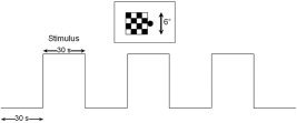
Experimental setup used for both EEG and fMRI recording sessions. Stimulus consisted of a 2‐Hz pattern‐reversal checkerboard in either the right or left visual field. Subjects were instructed to maintain fixation on a point in the center of the screen.
Electrophysiological Recordings and Data Analysis
The EEG was acquired using a 64 channel Ag/AgCl electrode cap (Neuroscan, El Paso, TX). Electrode placement followed the International 10‐20 System [Klem et al.,1999] and were all referenced to a frontal central electrode (FCz). An electrode placed at AFz was used as the common ground. Interelectrode impedances were kept below 10 kOhms. Horizontal and vertical eye movements were recorded using an electro‐oculogram (EOG) with electrodes placed over the outer canthus of the right and left eye as well as above and below the right eye. Subjects were comfortably seated in a soundproof, dimly lit room. EEG recordings were digitally recorded at 500 Hz with a bandpass of 0.1–100 Hz together with a 60‐Hz notch filter and stored for offline analysis.
Postprocessing was performed using the SCAN analysis software (Neuroscan). EEG epochs (−10 to 300 ms temporal range) were created based on the onset of triggers recorded during the recording session. The data were bandpass‐filtered within 1–35 Hz. An EOG artifact correction algorithm was used to remove all trials with amplitudes that exceed ±75 mV. The trials were detrended using a second‐order polynomial correction and then independently averaged for right and left stimulus conditions. This resulted in two VEP datasets (left hemifield and right hemifield) per participant. Each dataset consisted of at least 250 sweeps out of a maximum of 360, which is far greater than the minimum number of sweeps required for VEP analysis [Odom et al.,2004]. Subsequently, each dataset had a relatively large SNR (the SNR was calculated using the peak VEP amplitude and the prestimulus time interval).
VEP Source Analysis
Source analysis of VEP data was carried out using the CURRY V4.5 software (Neuroscan). Individually shaped realistic head models were created for each subject using a semiautomated boundary element algorithm [Fuchs et al.,1998]. These head models were tessellated with approximately 3,000 triangles per compartment with a triangle edge length of 8, 7, and 6 mm and conductivities of 0.33, 0. 0042, and 0.33 S/m for the scalp, skull, and brain regions, respectively. Electrode positions were determined by locating fiducial landmarks placed on the subject prior to fMRI scanning. A coordinate system using the vectors joining the right and left preauricular points (PAL, PAR) and Nasion (NAS) landmarks was created. In order to localize the generators of the pattern‐reversal stimulus, a single current dipole was used as a source model. This has been shown to be an appropriate source model for similar VEP studies [Slotnick et al.,1999; Steger et al.,2001]. In each participant dipole localization was carried out for both left and right hemifield datasets. A single current dipole was fitted at every time instant between 0–200 ms. The dipole position was initially seeded at the origin of the brain model (where the PAL/PAR and NAS vectors meet). The best‐fit dipole position and residual variance (RV) were calculated, as was its distance from the center of the fMRI cluster for each time instant. To determine how robust the inverse solution was, the inverse procedure was repeated by constraining dipole solutions to the visual cortex. This was done by segmenting the visual cortex with voxels that matched those used during fMRI recordings (Fig. 2). This resulted in approximately 2,000 elements per segmented volume. A dipole was placed at the center of each voxel and the best‐fit magnitude and orientation together with the residual variance was recorded. The center of VEP activity was calculated by retaining 1% of the solutions with the least variance and implementing a center of mass algorithm, using the location of each solution weighted by its explained variance.
Figure 2.
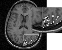
Segmentation of right visual cortex (magnification shown on right). The segmented volume was divided into a 3D grid of voxels with dimensions matching those used during fMRI recordings. Each voxel served as a testing site for possible left hemifield VEP dipole solutions. Similar segmentation was also done in the left visual cortex for right hemifield VEP dipole solutions (not shown here).
Functional MRI
Anatomical scans
fMRI recording sessions were made on a 1.5T unit (GE Signa, Milwaukee, WI) using a quadrature head coil. Prior to fMRI scanning, 120 high‐resolution axial images were taken using an inversion recovery sequence. The field of view (FOV) was 24 cm, resulting in slices with a 256 × 256 × 120 pixel dimension (pixel dimension = 0.937 × 0.937 × 1 mm) with a 0.5‐mm gap between axial slices.
Functional scans
A fast gradient echo imaging sequence with a spiral readout [Glover,1999] was employed for functional scans. The FOV was 24 cm, with a 64 × 64 pixel dimension along with a 5‐mm gap between axial slices (24 slices in total). Imaging parameters were as follows: TR/TE: 2,000/40 ms, flip angle: 90°, temporal points: 105. Headphones where placed on the subject to suppress noise from the switching gradients. Head padding was also used to suppress head movements. Prior to Fourier transformation, spiral k‐space data were regridded to Cartesian‐based coordinates [Glover,1999] giving a final voxel size of 3.75 × 3.75 × 5 mm. Spiral k‐space acquisition was used rather than a rectilinear trajectory because it is less sensitive to subtle motion, as it acquires the low spatial frequency information of k‐space first, resulting in greater BOLD contrast, relative to rectilinear (e.g., echoplanar imaging) methods [Noll et al.,1995].
fMRI analysis was carried out using AFNI software [Cox,1996]. Motion correction was carried out by registering all functional volumes to the first collected volume. The raw signal in each voxel was Fourier‐filtered with a bandpass of 0.15–2 Hz, detrended using a second‐order polynomial, then averaged across both trials. Correlation analysis was carried out using the processed fMRI signal with a boxcar stimulus profile. Correlation values below ±0.3 (P < 10−4) were discarded. These activation maps were smoothed using a Gaussian filter (full‐width at half‐maximum (FWHM) = 5 mm). The center of the activated cluster was computed with a center of mass algorithm, weighted by the correlation coefficient. This coordinate was ported into EEG source localization software for direct comparison (discussed below) with VEP source modeling estimates.
The group average N75 and P100 dipole positions were overlaid onto the group average fMRI dataset. Spherical regions of interest (ROIs) with a 7 mm radius were placed around these N75 and P100 locations. The fMRI signal over all voxels within these ROIs was extracted and graphically displayed (see Results). To investigate the correlation coefficient of the fMRI signal and stimulus profile as a function of distance between the N75 and P100 dipole positions, three ROIs were placed along the line joining the N75 and P100 positions. Correlation coefficient values within each ROI were averaged and graphically displayed.
RESULTS
VEP Data Analysis
The group average VEP scalp topography and the signal measured at electrode Oz from one participant during left and right hemifield stimulation is shown in Figure 3. The responses elicited the three main components associated with pattern reversal visual stimulation (latency values averaged over all participants and hemifields together with the standard deviations are in parentheses): N75 (74.2 ± 2.4 ms), P100 (107.8 ± 9.8 ms), and N150 (166.7 ± 21.2 ms). For all subjects, the N75 component was largest in electrodes ipsilateral to the stimulated field. The P100 component was maximal over the contralateral side of the stimulated field. To detect possible habituation in our data, the first 15 s of the VEP data recorded during stimulation was averaged and compared to the last 15 s. No significant difference in latency or amplitude was detected, indicating that neural habituation was not a factor in our measurements. These habituation results are in agreement with a similar study by Singh et al. [2003].
Figure 3.
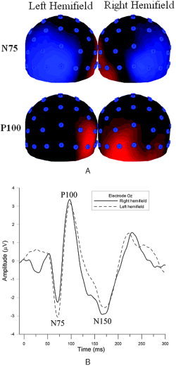
A: Occipital view of group average potential maps of N75 and P100 VEP components. Blue indicates negative potential, red indicates positive potential. Top row: N75 potential map during left and right hemifield stimulation. Bottom row: P100 potential map during left and right hemifield stimulation. B: VEP waveform measured from electrode site Oz from one participant. The dark line represents the VEP response obtained during right hemifield stimulation. The lighter dashed line is the VEP response obtained during left hemifield stimulation.
VEP and fMRI
Dipole locations of the N75 and P100 from one subject are displayed in Figure 4. Scalp topographies of the modeled N75 and P100 sources from the same subject are shown in Figure 5. fMRI activation maps averaged over all participants are shown in Figure 6. The combined dipole solutions and fMRI centers of activity (COA) averaged over all subjects are displayed in Figure 7. Details are listed in Table I. In all participants the voxels with the highest positive correlation coefficients were found near the most posterior portion of the calcarine fissure, contralateral to the stimulated visual field. Negative correlation values were also greatest on the contralateral side, anterior to the positive correlation values. We also investigated the possibility of fMRI signal habituation due to sustained prolonged visual stimulation. These effects were found to be minimal, and are consistent with previous studies using a reversing checkerboard stimulus [Howseman et al.,1998; Kruger et al.,1998]. For display purposes only, the results are superimposed on the MRI of one of the participants. The generator(s) representing the N150 component is not displayed (see Discussion).
Figure 4.
Dipole localization of N75 (orange dipole) and P100 (yellow dipole) from one participant during left and right hemifield stimulation.
Figure 5.
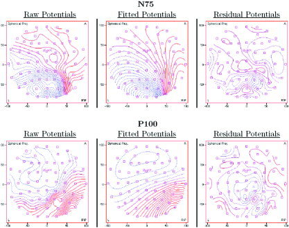
Overhead view of raw, fitted, and residual potential maps of the modeled N75 and P100 dipoles from one participant during left field stimulation. The raw potentials are shown on the left, the fitted potentials are shown in the middle, and the residual potentials are shown on the right. For this participant, the fitted maps of the N75 and P100 explained 94% and 96% of the raw maps, respectively.
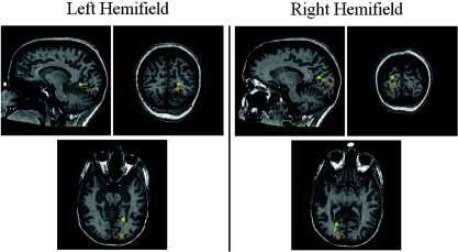
Figure 6.
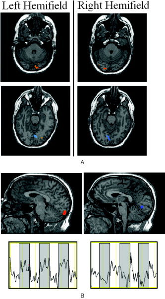
A: Axial views of fMRI group average maps showing the peak positive (red) and negative (blue) fMRI response during left and right hemifield stimulation. B: Sagittal view of group average fMRI maps showing the peak positive (red) and negative response (blue) during left field stimulation (results during right field stimulation are similar, and are not displayed). The mean fMRI signals extracted from the positive and negative ROI areas are displayed below their respective fMRI map. Gray bars indicate periods of visual stimulation. In both a and b, fMRI maps are thresholded to P ≤ 10−5.
Figure 7.
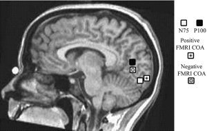
Mean localization over all subjects of N75 and P100 dipoles when using a realistic head model (white and black squares, respectively): Mean fMRI center of activity (COA) is shown for positive correlation (square with star) and negative correlation (square with circle). For display purposes only, results are superimposed on a mid‐sagittal MRI from one participant.
Table 1.
N75, P100, +BOLD and −BOLD COA locations averaged over all subjects (SD in parentheses)
| Left hemifield stimulation (x, y, z) | Right hemifield stimulation (x, y, z) | |
|---|---|---|
| N75 | −26.4, 61.3, 44.2 (11.7, 12.3, 18.5) | 7.5, 65.7, 49.6 (11.7, 11.3, 17.1) |
| P100 | −25.6, 52.0, 62.4 (7.5, 14.7, 11.3) | 9.5, 55.0, 53.1 (12.5, 17.2, 22.5) |
| +BOLD | −17.1, 69.3, 49.0 (11.7, 6.8, 5.5) | 23.3, 69.4, 46.6 (9.1, 11.6, 8.8) |
| −BOLD | −9.0, 54.9, 54.6 (5.9, 7.2, 7.6) | 6.5, 56.1, 48.1 (6.1, 8.7, 6.6) |
The coordinate system is defined via the preauricular points and the nasion of the subject. The positive x‐axis goes through the left preauricular point and the negative y‐axis goes through the nasion. The origin is located at the point where these two axes intersect, and the +z‐axis goes upwards from the origin, perpendicular to the x and y axis.
For the VEP, the y (running from anterior to posterior) and z (running from inferior to superior) coordinates of the N75 and P100 dipole positions were similar for left and right visual field stimulation, while the x (running from right to left) coordinate was significantly closer to midline during right visual field stimulation (P < 0.05). These VEP results were similar for both when the seed point was in the center of the brain and when limiting the inverse algorithm to the visual cortex. The sources of the VEP were localized in close proximity to the contralateral calcarine fissure, or near the primary visual cortex (V1). The N75 component was localized near the most posterior portion of the calcarine fissure. The P100 component was also localized near the calcarine fissure, although significantly more anterior to the N75 source (P < 0.05). The average explained variance between the modeled and measured potentials of the N75 and P100 source across all subjects and hemifields was 91% for the N75 and 94% for the P100. The mean distance between the N75 and P100 was approximately 2.5 ± 0.9 cm (Fig. 5).
For comparison with previous VEP localization studies, we also used a spherical head model for localizing the N75 and P100. Here, the N75 source location was comparable to that obtained when using a realistic model. The P100 location obtained by the spherical model was localized well outside V1, near V2/V3 (results not shown). This difference between results for spherical and realistic head models is not unexpected, since spherical models perform worse for sources deeper in the brain [Menninghaus et al.,1994; Tomita et al.,1996].
The fMRI signal averaged over all subjects, extracted from the ROI surrounding the N75 dipole location, is displayed in Figure 8. Mean fMRI correlation values as a function of distance between N75 and P100 dipole positions are displayed in Figure 9. The mean distance between the positive fMRI COA and negative fMRI COA was approximately 2.1 ± 1.3 cm. The location of positive and negative fMRI COA falls within the standard deviations of the mean N75 and P100 dipole position, respectively. Moreover, in 7 of the 8 subjects the N75 was closest to the positive fMRI COA, while the P100 was closest to the negative fMRI COA in five subjects. Overall, the mean distance between the N75 and positive fMRI COA was approximately 2.0 ± 1.0 cm, while the mean distance between the P100 and the negative fMRI COA was approximately 3.0 ± 1.6 cm.
Figure 8.
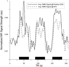
MR signal averaged over voxels within the ROI surrounding the positive fMRI COA (dark line) and N75 dipole location (light, dashed line). Black rectangles indicate periods of visual stimulation. See text for how ROI were constructed.
Figure 9.
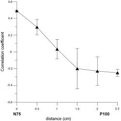
Mean fMRI correlation coefficient values from within the ROI placed along the line joining N75 and P100 dipole position with a separation of approximately 2.5 cm. Values are averaged over left and right field stimulation. The standard deviation is represented by the errors bars. This mean correlation coefficient is positive for N75, negative for P100.
DISCUSSION
Despite the large number of integrated ERP/fMRI studies, the spatial relationship of ERP and fMRI sources is still poorly understood. The most common approach to combine fMRI and ERP data is to constrain ERP dipole solutions to the area of activity obtained by fMRI [Ahlfors et al.,1999; Opitz et al.,1999]. This is advantageous from an inverse solution point of view, as it imposes limits on possible dipole solution sites and may also aid in better estimating the number of dipolar sources. This approach has been used in several VEP/fMRI studies [Di Russo et al.,2002,2005; Vanni et al.,2004]. However, this method strongly relies on the assumption that dipolar sources of ERP activity are indeed located within regions exhibiting a positive fMRI BOLD response. A VEP/fMRI study by Di Russo et al. [2002] reported a better correspondence between the location of the N75 dipole and the positive BOLD response than between the P100 dipole and the positive BOLD response. A similar study by Bonmassar et al. [2001] (using simultaneously acquired VEP/fMRI data) estimated the VEP generator site by using a 1) unconstrained and 2) fMRI‐constrained inverse algorithm. In the unconstrained approach, they found that the VEP cortical activity (collapsed over the entire VEP temporal window, and thus over the N75 and P100 components) was localized along the entire length of the calcarine sulcus. It should be noted that the aforementioned studies did not take into account the negative BOLD response, which may also correlate with certain ERP components.
A recent animal study by Kim et al. [2004] showed that, for relatively large voxels, the measured fMRI signal may accurately reflect the underlying neuronal activity. The measured ERP more directly reflects neuronal activity, but suffers from its limited spatial resolution, partly due to possible localization errors. In this study, localization errors were minimized by using subject specific VEP recordings with a high SNR, in conjunction with individually constructed realistic head models for dipole source modeling.
The results from this study provide strong support that the N75 generator is localized in area V1 of the visual cortex, confirming previous results [Di Russo et al.,2002; Shigeto et al.,1998; Tabuchi et al.,2002]. In particular, our results indicate that for a pattern‐reversal stimulus spanning 6° of the visual angle, the N75 source is located near the posterior portion of the calcarine fissure.
Several VEP reports have indicated that the P100 generator is located in area V1 [Shigeto et al.,1998; Tabuchi et al.,2002], but other VEP studies have argued that it may also originate in area V2/V3 [Onofrj et al.,1995], V3/V4 [Schroeder et al.,1995], and V5 [Di Russo et al.,2005]. Invasive studies using subdural electrodes by Noachtar et al. [1993] reported that the P100 is most probably generated by a dipole source localized in close proximity of the calcarine fissure. Our results also indicate that the P100 dipolar source is near the calcarine fissure, although significantly anterior (P < 0.01) and slightly superior (P < 0.1) to the N75 generator. The consistency of these findings across all subjects supports the hypothesis that the N75 and P100 sources are located in V1, although in substantially different locations along the calcarine fissure.
Localizing the N150 component has proven to be difficult in the past. Some reports [Di Russo et al.,2002,2005] suggest that there may be four dipoles needed to correctly model this source. Our study was limited to a sole dipole source model only, and consequently localization of the N150 component is left for further study.
Our fMRI results showed areas in the visual cortex consisting of significant positive and negative BOLD responses. The peak positive BOLD response was in the posterior portion of the calcarine fissure, contralateral to the stimulus field. This is consistent with similar studies [Engel et al.,1994; Janz et al.,2000]. A portion of the negative fMRI response was found on the ipsilateral side, but peaked on the contralateral side. This is similar to the findings of Smith et al. [2004].
In 7 of the 8 subjects, it was found that the dipole source in the 65–85 ms time range (N75) was localized closest to the peak positive fMRI activity. In the ROI surrounding the N75 dipole, we found voxels with a highly significant positive BOLD response. The correlation coefficient of the positive fMRI signal quickly decreased as it approached the more anterior P100 dipole position, which is consistent with previous fMRI studies using checkerboard stimulus [Janz et al.,2000]. The correlation becomes negative approximately halfway between the N75 and P100 dipole locations (Fig. 9). The area surrounding the P100 generator did not show any significant positive BOLD activity, but contained voxels that exhibited a negative BOLD response.
The results presented here suggest a strong correspondence between the location of the N75 generator and the positive BOLD response, but not for the P100 and the positive BOLD response as reported by Di Russo et al. [2002]. In this study, we found that in the majority of subjects the location of the P100 corresponded better to the location of the peak negative BOLD response.
Studies have indicated that the positive fMRI activity seen in BOLD‐based experiments is largely due to excitatory synaptic activity [Lauritzen,2005; Waldvogel et al.,2000; Wenzel et al.,2000]. Initial studies argued that the negative BOLD response is due to “vascular stealing” [Shmuel et al.,2002; Smith et al.,2000]. More recent studies have provided evidence against this hypothesis [Smith et al.,2004], suggesting that it is mainly due to neuronal inhibition [Kobayashi et al., 2005; Shmuel et al.,2003; Stefanovic et al.,2004]. Our study is consistent with this suggestion, as it has been suggested that the N75 and P100 represent excitatory and inhibitory processes, respectively [Thilo et al.,2003].
CONCLUSION
The cortical generators of the pattern‐reversal visual stimulus were studied using VEP and fMRI measurements. With subject‐specific data and realistic head models, we were able to reliably separate the generators of the N75 and P100 components to distinct areas of the primary visual cortex. In the majority of subjects the VEP/fMRI data indicate a correspondence between the location of the peak positive BOLD response and the N75 dipole location. The location of the P100, on the other hand, corresponded to an area of the brain containing a significant negative BOLD response. The results from this study also indicate that the negative BOLD response should be considered when comparing ERP and fMRI sources.
Acknowledgements
The authors thank Doug Wilson for theoretical contributions and Jeannine Gravel and Mark Given for support with EEG and fMRI measurements, respectively.
REFERENCES
- Ahlfors SP, Simpson GV, Dale AM, Belliveau JW, Liu AK, Korvenoja A, Virtanen J, Huotilainen M, Tootell RB, Aronen HJ, Ilmoniemi RJ (1999): Spatiotemporal activity of a cortical network for processing visual motion revealed by MEG and fMRI. J Neurophysiol 82: 2545–2555. [DOI] [PubMed] [Google Scholar]
- Arroyo S, Lesser RP, Poon WT, Webber WR, Gordon B (1997): Neuronal generators of visual evoked potentials in humans: visual processing in the human cortex. Epilepsia 38: 600–610. [DOI] [PubMed] [Google Scholar]
- Bonmassar G, Schwartz DP, Liu AK, Kwong KK, Dale AM, Belliveau JW (2001): Spatiotemporal brain imaging of visual‐evoked activity using interleaved EEG and fMRI recordings. Neuroimage 13: 1035–1043. [DOI] [PubMed] [Google Scholar]
- Cohen D, Cuffin BN, Yunokuchi K, Maniewski R, Purcell C, Cosgrove GR, Ives J, Kennedy JG, Schomer DL (1990): MEG versus EEG localization test using implanted sources in the human brain. Ann Neurol 28: 811–817. [DOI] [PubMed] [Google Scholar]
- Cox RW (1996): AFNI: software for analysis and visualization of functional magnetic resonance neuroimages. Comput Biomed Res 29: 162–173. [DOI] [PubMed] [Google Scholar]
- Cuffin BN, Cohen D, Yunokuchi K, Maniewski R, Purcell C, Cosgrove GR, Ives J, Kennedy J, Schomer D (1991): Tests of EEG localization accuracy using implanted sources in the human brain. Ann Neurol 29: 132–138. [DOI] [PubMed] [Google Scholar]
- Di Russo F, Martinez A, Sereno MI, Pitzalis S, Hillyard SA (2002): Cortical sources of the early components of the visual evoked potential. Hum Brain Mapp 15: 95–111. [DOI] [PMC free article] [PubMed] [Google Scholar]
- Di Russo F, Pitzalis S, Spitoni G, Aprile T, Patria F, Spinelli D, Hillyard SA (2005): Identification of the neural sources of the pattern‐reversal VEP. Neuroimage 24: 874–886. [DOI] [PubMed] [Google Scholar]
- Engel SA, Rumelhart DE, Wandell BA, Lee AT, Glover GH, Chichilnisky EJ, Shedler MN (1994): fMRI of human visual cortex. Nature 369: 525. [DOI] [PubMed] [Google Scholar]
- Ferguson AS, Stroink G (1997): Factors affecting the accuracy of the boundary element method in the forward problem. I. Calculating surface potentials. IEEE Trans Biomed Eng 44: 1139–1155. [DOI] [PubMed] [Google Scholar]
- Fortune B, Hood DC (2003): Conventional pattern‐reversal VEPs are not equivalent to summed multifocal VEPs. Invest Ophthalmol Vis Sci 44: 1364–1375. [DOI] [PubMed] [Google Scholar]
- Fuchs M, Drenckhahn R, Wischmann HA, Wagner M (1998): An improved boundary element method for realistic volume‐conductor modeling. IEEE Trans Biomed Eng 45: 980–997. [DOI] [PubMed] [Google Scholar]
- Fuchs M, Wagner M, Kastner J (2001): Boundary element method volume conductor models for EEG source reconstruction. Clin Neurophysiol 112: 1400–1407. [DOI] [PubMed] [Google Scholar]
- Glover GH (1999): Simple analytic spiral K‐space algorithm. Magn Reson Med 42: 412–415. [DOI] [PubMed] [Google Scholar]
- Grimm C, Schreiber A, Kristeva‐Feige R, Mergner T, Hennig J, Lucking CH (1998): A comparison between electric source localisation and fMRI during somatosensory stimulation. Electroencephalogr Clin Neurophysiol 106: 22–29. [DOI] [PubMed] [Google Scholar]
- Howseman AM, Porter DA, Hutton C, Josephs O, Turner R (1998): Blood oxygenation level dependent signal time courses during prolonged visual stimulation. Magn Reson Imaging 16: 1–11. [DOI] [PubMed] [Google Scholar]
- Janz C, Schmitt C, Speck O, Hennig J (2000): Comparison of the hemodynamic response to different visual stimuli in single‐event and block stimulation fMRI experiments. J Magn Reson Imaging 12: 708–714. [DOI] [PubMed] [Google Scholar]
- Kim DS, Ronen I, Olman C, Kim SG, Ugurbil K, Toth LJ (2004): Spatial relationship between neuronal activity and BOLD functional MRI. Neuroimage 21: 876–885. [DOI] [PubMed] [Google Scholar]
- Klem GH, Luders HO, Jasper HH, Elger C (1999): The ten‐twenty electrode system of the International Federation. The International Federation of Clinical Neurophysiology. Electroencephalogr Clin Neurophysiol Suppl 52: 3–6. [PubMed] [Google Scholar]
- Kobayashi E, Bagshaw AP, Grova C, Dubeau F, Gotman J (2006): Negative BOLD responses to epileptic spikes. Hum Brain Mapp 27: 488–497. [DOI] [PMC free article] [PubMed] [Google Scholar]
- Kruger G, Kleinschmidt A, Frahm J (1998): Stimulus dependence of oxygenation‐sensitive MRI responses to sustained visual activation. NMR Biomed 11: 75–79. [DOI] [PubMed] [Google Scholar]
- Kruggel F, Wiggins CJ, Herrmann CS, von Cramon DY (2000): Recording of the event‐related potentials during functional MRI at 3.0 Tesla field strength. Magn Reson Med 44: 277–282. [DOI] [PubMed] [Google Scholar]
- Kurita‐Tashima S, Tobimatsu S, Nakayama‐Hiramatsu M, Kato M (1991): Effect of check size on the pattern reversal visual evoked potential. Electroencephalogr Clin Neurophysiol 80: 161–166. [DOI] [PubMed] [Google Scholar]
- Lauritzen M (2005): Reading vascular changes in brain imaging: is dendritic calcium the key? Nat Rev Neurosci 6: 77–85. [DOI] [PubMed] [Google Scholar]
- Meijs JW, Weier OW, Peters MJ, van Oosterom A (1989): On the numerical accuracy of the boundary element method. IEEE Trans Biomed Eng 36: 1038–1049. [DOI] [PubMed] [Google Scholar]
- Menninghaus E, Lutkenhoner B, Gonzalez SL (1994): Localization of a dipolar source in a skull phantom: realistic versus spherical model. IEEE Trans Biomed Eng 41: 986–989. [DOI] [PubMed] [Google Scholar]
- Menon V, Ford JM, Lim KO, Glover GH, Pfefferbaum A (1997): Combined event‐related fMRI and EEG evidence for temporal‐parietal cortex activation during target detection. Neuroreport 8: 3029–3037. [DOI] [PubMed] [Google Scholar]
- Mulert C, Jager L, Schmitt R, Bussfeld P, Pogarell O, Moller HJ, Juckel G, Hegerl U (2004): Integration of fMRI and simultaneous EEG: towards a comprehensive understanding of localization and time‐course of brain activity in target detection. Neuroimage 22: 83–94. [DOI] [PubMed] [Google Scholar]
- Noachtar S, Hashimoto T, Luders H (1993): Pattern visual evoked potentials recorded from human occipital cortex with chronic subdural electrodes. Electroencephalogr Clin Neurophysiol 88: 435–446. [DOI] [PubMed] [Google Scholar]
- Noll DC, Cohen JD, Meyer CH, Schneider W (1995): Spiral K‐space MR imaging of cortical activation. J Magn Reson Imaging 5: 49–56. [DOI] [PubMed] [Google Scholar]
- Odom JV, Bach M, Barber C, Brigell M, Marmor MF, Tormene AP, Holder GE, Vaegan (2004): Visual evoked potentials standard (2004): Doc Ophthalmol 108: 115–123. [DOI] [PubMed] [Google Scholar]
- Ogawa S, Tank DW, Menon R, Ellermann JM, Kim SG, Merkle H, Ugurbil K (1992): Intrinsic signal changes accompanying sensory stimulation: functional brain mapping with magnetic resonance imaging. Proc Natl Acad Sci U S A 89: 5951–5955. [DOI] [PMC free article] [PubMed] [Google Scholar]
- Onofrj M, Fulgente T, Thomas A, Curatola L, Peresson M, Lopez L, Locatelli T, Martinelli V, Comi G (1995): Visual evoked potentials generator model derived from different spatial frequency stimuli of visual field regions and magnetic resonance imaging coordinates of V1, V2, V3 areas in man. Int J Neurosci 83: 213–239. [DOI] [PubMed] [Google Scholar]
- Opitz B, Mecklinger A, Von Cramon DY, Kruggel F (1999): Combining electrophysiological and hemodynamic measures of the auditory oddball. Psychophysiology 36: 142–147. [DOI] [PubMed] [Google Scholar]
- Roth BJ, Balish M, Gorbach A, Sato S (1993): How well does a three‐sphere model predict positions of dipoles in a realistically shaped head? Electroencephalogr Clin Neurophysiol 87: 175–184. [DOI] [PubMed] [Google Scholar]
- Schroeder CE, Steinschneider M, Javitt DC, Tenke CE, Givre SJ, Menta AD, Simpson GV, Arezzo JC, Vaughan HG (1995): Localization of ERP generators and identification of underlying neural processes. Electroencephalogr Clin Neurophysiol Suppl 44: 55–75. [PubMed] [Google Scholar]
- Shigeto H, Tobimatsu S, Yamamoto T, Kobayashi T, Kato M (1998): Visual evoked cortical magnetic responses to checkerboard pattern reversal stimulation: a study on the neural generators of N75, P100 and N145. J Neurol Sci 156: 186–194. [DOI] [PubMed] [Google Scholar]
- Shmuel A, Yacoub E, Pfeuffer J, Van de Moortele PF, Adriany G, Hu X, Ugurbil K (2002): Sustained negative BOLD, blood flow and oxygen consumption response and its coupling to the positive response in the human brain. Neuron 36: 1195–1210. [DOI] [PubMed] [Google Scholar]
- Shmuel A, Augath M, Rounis E, Logothetis N, Smirknakis S (2003): Negative BOLD repsonse ipsilateral to the visual stimulus: origin is not blood stealing. Neuroimage 19(Suppl): 309. [Google Scholar]
- Singh M, Kim S, Kim TS (2003): Correlation between BOLD‐fMRI and EEG signal changes in response to visual stimulus frequency in humans. Magn Reson Med 49: 108–114. [DOI] [PubMed] [Google Scholar]
- Slotnick SD, Klein SA, Carney T, Sutter E, Dastmalchi S (1999): Using multi‐stimulus VEP source localization to obtain a retinotopic map of human primary visual cortex. Clin Neurophysiol 110: 1793–1800. [DOI] [PubMed] [Google Scholar]
- Smith AT, Singh KD, Greenlee MW (2000): Attentional suppression of activity in the human visual cortex. Neuroreport 11: 271–277. [DOI] [PubMed] [Google Scholar]
- Smith AT, Williams AL, Singh KD (2004): Negative BOLD in the visual cortex: evidence against blood stealing. Hum Brain Mapp 21: 213–220. [DOI] [PMC free article] [PubMed] [Google Scholar]
- Stefanovic B, Warnking JM, Pike GB (2004): Hemodynamic and metabolic responses to neuronal inhibition. Neuroimage 22: 771–778. [DOI] [PubMed] [Google Scholar]
- Steger J, Imhof K, Denoth J, Pascual‐Marqui RD, Steinhausen HC, Brandeis D (2001): Brain mapping of bilateral visual interactions in children. Psychophysiology 38: 243–253. [PubMed] [Google Scholar]
- Tabuchi H, Yokoyama T, Shimagowara M, Shiraki K, Nagasaka E, Miki T (2002): Study of the visual evoked magnetic field with the m‐sequence technique. Invest Ophthalmol Vis Sci 43: 2045–2054. [PubMed] [Google Scholar]
- Thilo KV, Kleinschmidt A, Gresty MA (2003): Perception of self‐motion from peripheral optokinetic stimulation suppresses visual evoked responses to central stimuli. J Neurophysiol 90: 723–730. [DOI] [PubMed] [Google Scholar]
- Tomita S, Kajihara S, Kondo Y, Yoshida Y, Shibata K, Kado H (1996): Influence of head model in biomagnetic source localization. Brain Topogr 8: 337–340. [DOI] [PubMed] [Google Scholar]
- Vanni S, Warnking J, Dojat M, Delon‐Martin C, Bullier J, Segebarth C (2004): Sequence of pattern onset responses in the human visual areas: an fMRI constrained VEP source analysis. Neuroimage 21: 801–817. [DOI] [PubMed] [Google Scholar]
- Vanrumste B, Van Hoey G, Van de Walle R, D'Have MR, Lemahieu IA, Boon PA (2002): Comparison of performance of spherical and realistic head models in dipole localization from noisy EEG. Med Eng Phys 24: 403–418. [DOI] [PubMed] [Google Scholar]
- Vitacco D, Brandeis D, Pascual‐Marqui R, Martin E (2002): Correspondence of event‐related potential tomography and functional magnetic resonance imaging during language processing. Hum Brain Mapp 17: 4–12. [DOI] [PMC free article] [PubMed] [Google Scholar]
- Waldvogel D, van Gelderen P, Muellbacher W, Ziemann U, Immisch I, Halle HM (2000): The relative metabolic demand of inhibition and excitation. Nature 406: 995–998. [DOI] [PubMed] [Google Scholar]
- Wenzel R, Wobst P, Heekeren HH, Kwong KK, Brandt SA, Kohl M, Obrig H, Dirnagl U, Villringer A (2000): Saccadic suppression induces focal hypooxygenation in the occipital cortex. J Cereb Blood Flow Metab 20: 1103–1110. [DOI] [PubMed] [Google Scholar]
- Whittingstall K, Stroink G, Gates L, Connolly JF, Finley A (2003): Effects of dipole position, orientation and noise on the accuracy of EEG source localization. Biomed Eng Online 2: 14. [DOI] [PMC free article] [PubMed] [Google Scholar]