Bayesian estimation of evoked and induced responses

Abstract

We describe an extension of our empirical Bayes approach to magnetoencephalography/electroencephalography (MEG/EEG) source reconstruction that covers both evoked and induced responses. The estimation scheme is based on classical covariance component estimation using restricted maximum likelihood (ReML). We have focused previously on the estimation of spatial covariance components under simple assumptions about the temporal correlations. Here we extend the scheme, using temporal basis functions to place constraints on the temporal form of the responses. We show how the same scheme can estimate evoked responses that are phase‐locked to the stimulus and induced responses that are not. For a single trial the model is exactly the same. In the context of multiple trials, however, the inherent distinction between evoked and induced responses calls for different treatments of the underlying hierarchical multitrial model. We derive the respective models and show how they can be estimated efficiently using ReML. This enables the Bayesian estimation of evoked and induced changes in power or, more generally, the energy of wavelet coefficients. Hum Brain Mapp, 2006. © 2006 Wiley‐Liss, Inc.

INTRODUCTION

Many approaches to the inverse problem acknowledge non‐uniqueness or uncertainty about any particular solution; a nice example of this is multistart spatiotemporal localization [Huang et al.,1998]. Bayesian approaches accommodate this uncertainty by providing a conditional density on an ensemble of possible solutions. Indeed, the approach described in this article is a special case of “ensemble learning” [Dietterich,2000] because the variational free energy (minimized in ensemble learning) and the restricted maximum likelihood (ReML) objective function (used below) are the same thing under a linear model. Recently, uncertainty has been addressed further by Bayesian model averaging over different solutions and forward models [Trujillo‐Barreto et al.,2004]. The focus of this article is on computing the dispersion or covariance of the conditional density using computationally efficient, analytic techniques. This approach eschews stochastic or complicated descent schemes by making Gaussian assumptions about random effects in the forward model.

In a series of previous communications we have introduced a solution to the inverse problem of estimating distributed sources causing observed responses in magnetoencephalography (MEG) or electroencephalography (EEG) data. The ill‐posed nature of this problem calls for constraints, which enter as priors, specified in terms of covariance components. By formulating the forward model as a hierarchical system one can use empirical Bayes to estimate these priors. This is equivalent to partitioning the covariance of observed data into observation error and a series of components induced by prior source covariances. This partitioning uses ReML estimates of the covariance components. The ensuing scheme has a number of advantages in relation to alternative approaches such as “L‐Curve” analysis. First, it provides a principled and unique estimation of the regularization, implicit in all inverse solutions to distributed sources [Phillips et al.,2005]. Second, it accommodates multiple priors, which are balanced in an optimal fashion (to maximize the evidence or likelihood of the data) [Phillips et al.,2005]. Third, the role of different priors can be evaluated in terms of the evidence of different models using Bayesian model comparison [Mattout et al., submitted]. Finally, the scheme is computationally efficient, requiring only the inversion of c × c matrices where c is the number of channels.

Because the scheme is based on covariance component estimation, it operates on second‐order data matrices (e.g., sample covariance matrices). Usually these matrices summarize covariances over peristimulus time. Current implementations of ReML in this context make some simplifying assumptions about the temporal correlations. In this work, we revisit these assumptions and generalize the previous scheme to accommodate temporal constraints that assure the conditional separability of the spatial and temporal responses. This separability means one can use the covariance of the data over time to give very precise covariance component estimates. Critically, this estimation proceeds in low‐dimensional channel space. After ReML, the covariance components specify matrices that are used to compute the conditional means and covariances of the underlying sources.

To date, the ReML estimates have been used to construct conditional (maximum a posteriori) estimates of the sources at a particular time. We show below that the same framework can easily provide images of energy expressed in any time‐frequency window, for example oscillations in the 5–25‐Hz frequency band from 150–200 msec during a face perception task [Henson et al.,2005a]. The analysis of both evoked responses that are time‐locked to trial onset and induced responses that are not use exactly the same model for a single trial; however, temporal priors on evoked and induced responses are fundamentally different for multiple trials. This is because there is a high correlation between the response evoked in one trial and that of the next. Conversely, induced responses have a random phase‐relationship over trials and are, a priori, independent. We will consider the implication these differences have for the ReML scheme and the way data are averaged before estimation.

This work comprises five sections. In the first we briefly reprise the ReML identification of conditional operators based on covariances over time for a single trial. We then consider an extension of this scheme that accommodates constraints on the temporal expression of responses using temporal basis functions. In the third section we show how the same conditional operator can be used to estimate response energy or power. In the fourth section we consider extensions to the model that cover multiple trials and show that evoked responses are based on the covariance of the average response over trials, whereas global and induced responses are based on the average covariance. In the fifth section we illustrate the approach using toy and real data.

Basic ReML Approach to Distributed Source Reconstruction

Hierarchical linear models

This section has been covered fully in our earlier descriptions, so we focus here on the structure of the problem and on the nature of the variables that enter the ReML scheme. The empirical Bayes approach to multiple priors in the context of unknown observation noise rests on the hierarchical observation model

(1)

where y represents a c × t data matrix of channels × time bins. L is a c × s lead‐field matrix, linking the channels to the s sources, and j is an s × t matrix of source activity over peristimulus time. ε⁽¹⁾ and ε⁽²⁾ are random effects, representing observation error or noise and unknown source activity, respectively. V ⁽¹⁾and V ⁽²⁾ are the temporal correlation matrices of these random effects. In our previous work we have assumed them to be the identity matrix; however, they could easily model serial correlations and indeed non‐stationary components. C ⁽¹⁾and C ⁽²⁾ are the spatial covariances for noise and sources, respectively; they are linear mixtures of covariance components Q ${}_{\mathit{\text{i}}}^{\text{(1)}}$ and Q ${}_{\mathit{\text{i}}}^{\text{(2)}}$ that embody spatial constraints on the solution. V ⁽¹⁾ ⊗ C ⁽¹⁾ represents a parametric noise covariance model [Huizenga et al.,2002] in which the temporal and spatial components factorize. Here the spatial component can have multiple components estimated through λ${}_{\mathit{\text{i}}}^{\text{(1)}}$, whereas the temporal form is fixed. At the second level, V ⁽²⁾ ⊗ C ⁽²⁾ can be regarded as spatiotemporal priors on the sources p(j) = N(0, V ⁽²⁾ ⊗ C ⁽²⁾), whose spatial components are estimated empirically in terms of λ${}_{\mathit{\text{i}}}^{\text{(2)}}$.

The ReML scheme described here is based on the two main results for vec operators and Kronecker tensor products

(2)

The vec operator stacks the columns of a matrix on top of each other to produce a long column vector. The trace operator tr(A) sums the leading diagonal elements of a matrix A and the Kronecker tensor product A ⊗ B replaces each element A _ij of A with A _ij B to produce a larger matrix. These equalities enable us to express the forward model in equation (1) as

(3)

and express the conditional mean ĵ and covariance as

(4)

The first and second lines of equation (4) are equivalent by the matrix inversion lemma. The conditional mean vec(ĵ) or maximum a posteriori (MAP) estimate is the most likely source, given the data. The conditional covariance encodes uncertainty about vec(j) and can be regarded as the dispersion of a distribution over an ensemble of solutions centered on the conditional mean.

In principle, equation (4) provides a viable way of computing conditional means of the sources and their conditional covariances; however, it entails pre‐multiplying a very long vector with an enormous (st × ct) matrix. Things are much simpler when the temporal correlations of noise and signal are the same i.e., V ⁽¹⁾ = V ⁽²⁾ = V. In this special case, we can compute the conditional mean and covariances using much smaller matrices.

(5)

Here M is a (s × c) matrix that corresponds to a MAP operator that maps the data to the conditional mean. This compact form depends on assuming the temporal correlations V of the observation error and the sources are the same. This ensures the covariance of the data cov(vec(y)) = Σ and the sources conditioned on the data factorize into separable spatial and temporal components

(6)

This is an important point because equation (6) is not generally true if the temporal correlations of the error and the sources are different, i.e., V ⁽¹⁾ ≠ V ⁽²⁾. Even if a priori there is no interaction between the temporal and spatial responses, a difference in the temporal correlations from the two levels induces conditional spatiotemporal dependencies. This means that the conditional estimate of the spatial distribution changes with time. This dependency precludes the factorization implicit in equation (5) and enforces a full‐vectorized spatiotemporal analysis equation (4), which is computationally expensive.

For the moment, we will assume the temporal correlations are the same and then generalize the approach in the next section for some special cases of V ⁽¹⁾ ≠ V ⁽²⁾.

Estimating the covariances

Under the assumption that V ⁽¹⁾ = V ⁽²⁾ = V, the only quantities that need to be estimated are the covariance components in equation (1). This proceeds using an iterative ReML scheme in which the covariance parameters maximize the log‐likelihood or log‐evidence

(7)

In brief, the λ = REML(A,B) operator decomposes a sample covariance matrix A into a number of specified components B = {B ₁, …} so that A ≈ ∑_i λ_i B _i. The ensuing covariance parameters λ = {λ_i,…} render the sample covariance the most likely. In our application, the sample covariance is simply the outer product of the vectorized data vec(y)vec(y)^T and the components are V ⊗ Q _i. Here, Q = {Q ${}_{\text{1}}^{\text{(1)}}$, …, LQ ${}_{\text{1}}^{\text{(2)}}$ L ^T, …} are the spatial covariance components from the first level of the model and the second level after projection onto channel space through the lead‐field.

ReML was originally formulated in terms of covariance component analysis but is now appreciated as a special case of expectation maximization (EM). The use of the ReML estimate properly accounts for the degrees of freedom lost in estimating the model parameters (i.e., sources) when estimating the covariance components. The “restriction” means that the covariance component estimated is restricted to the null space of the model. This ensures that uncertainty about the source estimates is accommodated in the covariance estimates. The details of ReML do not concern us here (they can be found in Friston et al. [2002] and Phillips et al. [2005]). The key thing is how the data enter the log‐likelihood that is maximized by ReML1

(8)

The second line uses the results in equation (2) and shows that the substitutions vec(y)vec(y)^T → yV ⁻¹ y ^T/rank(V) and V ⊗ Q → Q do not change the maximum of the objective function. This means we can replace the ReML arguments in equation (7) with much smaller (c × c) matrices.

(9)

Assuming the data are zero mean, this second‐order matrix yV ⁻¹ y ^T/rank(V) is simply the sample covariance matrix of the whitened data over the t time bins, where rank(V) = t. The greater the number of time bins, the more precise is the ReML covariance component estimators.

This reformulation of the ReML scheme requires the temporal correlations of the observation error and the sources to be the same. This ensures Σ = V ⊗ C can be factorized and affords the computational saving implicit in equation (9). There is no reason, however, to assume that the processes generating the signal and noise have the same temporal correlations. In the next section we finesse this unlikely assumption by restricting the estimation to a subspace defined by temporal basis functions.

A Temporally Informed Scheme

In this section we describe a simple extension to the basic ReML approach that enables some constraints to be placed on the form of evoked or induced responses. This involves relaxing the assumption that V ⁽¹⁾ = V ⁽²⁾. The basic idea is to project the data onto a subspace (via a matrix S) in which the temporal correlation of signal and noise are rendered formally equivalent. This falls short of a full spatiotemporal model but retains the efficiency of ReML scheme above and allows for differences between V ⁽¹⁾ and V ⁽²⁾ subject to the constraint that S ^T V ⁽²⁾ S = S ^T V ⁽¹⁾ S.

In brief, we have already established a principled and efficient Bayesian inversion of the inverse problem for EEG and MEG using ReML. To extend this approach to multiple time bins we need to assume that the temporal correlations of channel noise and underling sources are the same. In reality, sources are generally smoother than noise because of the generalized convolution implicit in synaptic and population dynamics at the neuronal level [Friston,2000]. By projecting the time‐series onto a carefully chosen subspace, however, we can make the temporal correlations of noise and signal formally similar. This enables us to solve a spatiotemporal inverse problem using the reformulation of the previous section. Heuristically, this projection removes high‐frequency noise components so that the remaining smooth components exhibit the same correlations as signal. We now go through the math that this entails.

Consider the forward model, where for notional simplicity V ⁽¹⁾ = V:

(10)

This is the same as equation (1) with the substitution j = kS ^T. The only difference is that the sources are estimated in terms of the activity k of temporal modes. The orthonormal columns of the temporal basis set S define these modes where S ^T S = I _r. When S has fewer columns than rows r < t, it defines an r‐subspace in which the sources lie. In other words, the basis set allows us to preclude temporal response components that are, a priori, unlikely (e.g., very high frequency responses or responses before stimulus onset). This restriction enables one to define a signal that lies in the subspace of the errors.

In short, the subspace S encodes prior beliefs about when and how signal will be evoked. They specify temporal priors on the sources through V ⁽²⁾ = SS ^T V ⁽¹⁾ SS ^T. This ensures that S ^T V ⁽²⁾ S = S ^T V ⁽¹⁾ S because S ^T S = I _r and renders the restricted temporal correlations formally equivalent. We will see later that the temporal priors on sources are also their posteriors, V ⁽²⁾ = V̂ because the temporal correlations are treated as fixed and known.

The restricted model can be transformed into a spatiotemporally separable form by post‐multiplying the first line of equation (10) by S to give

(11)

In this model, the temporal correlations of signal and noise are now the same. This restricted model has exactly the same form as equation (1) and can be used to provide ReML estimates of the covariance components in the usual way, using equation (9)

(12)

These are then used to compute the conditional moments of the sources as a function of time

(13)

The temporal correlations V̂ are rank deficient and non‐stationary because the conditional responses do not span the null space of S. This scheme does not represent a full spatiotemporal analysis; it is simply a device to incorporate constraints on the temporal component of the solution. A full analysis would require covariances that could not be factorized into spatial and temporal factors. This would preclude the efficient use of ReML covariance estimation described above. In most applications, however, a full temporal analysis would proceed using the above estimates from different trial types and subjects [e.g., see Kiebel and Friston,2004b].

In the examples in the section about applications, we specify S as the principal eigenvector of a temporal prior source covariance matrix based on a windowed autocorrelation (i.e., Toeplitz) matrix. In other words, we took a Gaussian autocorrelation matrix and multiplied the rows and columns with a window‐function to embody our a priori assumption that responses are concentrated early in peristimulus time. The use of prior constraints in this way is very similar to the use of anatomically informed basis functions to restrict the solution space anatomically [see Phillips et al.,2002]. Here, S can be regarded as a temporally informed basis set that defines a signal subspace.

Estimating Response Energy

In this section we consider the estimation of evoked and induced responses in terms of their energy or power. The energy is simply the squared norm (i.e., squared length) of the response projected onto some time‐frequency subspace defined by W. The columns of W correspond to the columns of a [wavelet] basis set that encompasses time‐frequencies of interest; for example, a sine–cosine pair of windowed sinusoids of a particular frequency. We deal first with estimating the energy of a single trial and then turn to multiple trials. The partitioning of energy into evoked and induced components pertains only to multiple trials.

For a single trial the energy expressed by the ith source is

(14)

where j _i,• is the ith row of the source matrix over all time bins. The conditional expectation of this energy obtains by averaging over the conditional density of the sources. The conditional density for the ith source over time is

(15)

and the conditional expectation of the energy is

(16)

Note that this is a function of yGy ^T, the corresponding energy in channel space E _y. The expression in equation (16) can be generalized to cover all sources, although this would be a rather large matrix to interpret

(17)

The matrix Ê is the conditional expectation of the energy over sources. The diagonal terms correspond to energy at the corresponding source (e.g., spectral density if W comprised sine and cosine functions). The off‐diagonal terms represent cross energy (e.g., cross‐spectral density or coherence).

Equation (17) means that the conditional energy has two components, one attributable to the energy in the conditional mean (the first term) and one related to conditional covariance (the second). The second component may seem a little counterintuitive: it suggests that the conditional expectation of the energy increases with conditional uncertainty about the sources. In fact, this is appropriate; when conditional uncertainty is high, the priors shrink the conditional mean of the sources toward zero. This results in an underestimate of energy based solely on the conditional expectations of the sources. By including the second term the energy estimator becomes unbiased. It would be possible to drop the second term if conditional uncertainty was small. This would be equivalent to approximating the conditional density of the sources with a point mass over its mean. The advantage of this is that one does not have to compute the s × s conditional covariance of the sources. However, we will assume the number of sources is sufficiently small to use equation (17).

In this section we have derived expressions for the conditional energy of a single trial. In the next section we revisit the estimation of response energy over multiple trials. In this context, there is a distinction between induced and evoked energy.

Averaging Over Trials

With multiple trials we have to consider trial‐to‐trial variability in responses. Conventionally, the energy associated with between‐trial variations, around the average or evoked response, is referred to as induced. Induced responses are normally characterized in terms of the energy of oscillations within a particular time‐frequency window. Because by definition they do not show a systematic phase relationship with the stimulus, they are expressed in the average energy over trials but not in the energy of the average. In this article, we use the term global response in reference to the total energy expressed over trials and partition this into evoked and induced components. In some formulations, a third component due to stationary, ongoing activity is considered. Here, we will subsume this component under induced energy. This is perfectly sensible, provided induced responses are compared between trials when ongoing or baseline power cancels.

Multitrial models

Hitherto we have dealt with single trials. When dealing with multiple trials, the same procedures can be adopted but there is a key difference for evoked and induced responses. The model for n trials is

(18)

where 1_n = [1,…1] is a 1 × n vector and Y = [y ₁…y _n represents data concatenated over trials. The multiple trials induce a third level in the hierarchical model. In this three‐level model, sources have two components: a component that is common to all trials k ⁽²⁾ and a trial‐specific component ε⁽²⁾. These are related to evoked and induced response components as follows.

Operationally we can partition the responses k ⁽¹⁾ in source space into a component that corresponds to the average response over trials, the evoked response, and an orthogonal component, the induced response.

(19)

where 1${}_{\mathit{\text{n}}}^{\text{−}}$ = [1/n, …, 1/n]^T is the generalized inverse of 1_n and is simply an averaging vector. As the number of trials n increases, the random terms at the second level are averaged away and the evoked response k ^(e) → k ⁽²⁾ approximates the common component. Similarly, the induced response k ⁽ⁱ⁾ → ε⁽²⁾ becomes the trial‐specific component. With the definition of evoked and induced components in place we can now turn to their estimation.

Evoked responses

The multitrial model can be transformed into a spatio‐temporally‐separable form by simply averaging the data Y = Y(1${}_{\mathit{\text{n}}}^{\text{−}}$ ⊗ I _t) and projecting onto the signal subspace. This is exactly the same restriction device used above to accommodate temporal basis functions but applied here to the trial‐average. This corresponds to post multiplying the first level by the trial‐averaging and projection operator 1${}_{\mathit{\text{n}}}^{\text{−}}$ ⊗ S to give

(20)

Here C ⁽¹⁾ = (1/n)C ⁽¹⁾ and C ^(e) = (1/n)C ⁽²⁾ + C ⁽³⁾ is a mixture of trial‐specific and nonspecific spatial covariances. This model has exactly the same form as the single‐trial model; enabling ReML estimation of C ⁽¹⁾ and C ^(e) that are needed to form the conditional estimator M (see equation [4])

(21)

The conditional expectation of the evoked response amplitude (e.g., event‐related potential [ERP], or event‐related field [ERF]) is simply

(22)

The conditional expectation of evoked power is then

(23)

where E ${}_{\text{y}}^{\text{(e)}}$ is the evoked cross‐energy in channel space. In short, this is exactly the same as a single‐trial analysis but using the channel data averaged over trials. This averaging is not appropriate, however, for the induced responses considered next.

Induced responses

To isolate and characterize induced responses, we effectively subtract the evoked response from all trials to give Ỹ = Y((I _n − 1${}_{\mathit{\text{n}}}^{\text{−}}$1_n) ⊗ I _t), and project this mean‐corrected data onto the signal subspace. The average covariance of the ensuing data is used and then decomposed using ReML. This entails post‐multiplying the first level of the multitrial model by (I _n − 1${}_{\mathit{\text{n}}}^{\text{−}}$1_n) ⊗ S to give

(24)

In this transformation k ⁽ⁱ⁾ is a large s × nr matrix that covers all trials. Again this model has the same spatiotemporally separable form as the previous models, enabling an efficient ReML estimation of the covariance components of C̃⁽¹⁾ and C ⁽ⁱ⁾

(25)

The first argument of the ReML function is just the covariance of the whitened, mean‐corrected data averaged over trials. The conditional expectation of induced energy, per trial, is then

(26)

where E ${}_{\mathit{\text{y}}}^{\text{(}\mathit{\text{i}}\text{)}}$ is the induced cross‐energy per trial, in channel space. The spatial conditional projector M and covariance Ĉ are defined as above (equations [22] and [23]). Although it would be possible to estimate the amplitude of induced responses for each trial, this is seldom interesting.

Summary

The key thing to take from this section is that the estimation of evoked responses involves averaging over trials and estimating the covariance components. Conversely, the analysis of induced responses involves estimating covariance components and then averaging. In both cases, the iterative ReML scheme operates on small c × c matrices.

The various uses of the ReML scheme and conditional estimators are shown schematically in Figure 1. All applications, be they single trial or trial averages, estimates of evoked responses, or induced energy, rest on a two‐stage procedure in which ReML covariance component estimators are used to form conditional estimators of the sources. The second thing to take from this figure is that the distinction between evoked and induced responses only has meaning in the context of multiple trials. This distinction rests on an operational definition, established in the decomposition of response energy in channel space. The corresponding decomposition in source space affords the simple and efficient estimation of evoked and induced power described in this section. Interestingly, however, conditional estimators of evoked and induced components are not estimates of the fixed k ⁽²⁾ and random ε⁽²⁾ effects in the hierarchical model. These estimates would require a full mixed‐effects analysis. This will be the subject of a subsequent article. Another interesting issue is that evoked and induced responses in channel space (where there is no estimation per se) represent a bi‐partitioning of global responses. This is not the case for their conditional estimates in source space. In other words, the conditional estimate of global power is not necessarily the sum of the conditional estimates of evoked and induced power.

Figure 1.

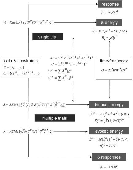
Restricted maximum likelihood (ReML) scheme. Schematic showing the various applications of the ReML scheme in estimating evoked and induced responses in multiple trials. See main text for an explanation of the variables.

Applications

In this section we illustrate the above procedures using toy and real data. The objective of the toy example is to clarify the nature of the operators and matrices, to highlight the usefulness of restricting the signal space and to show algorithmically how evoked and induced responses are recovered. The real data are presented to establish a degree of face validity, given that face‐related responses have been fully characterized in term of their functional anatomy. The toy example deals with the single‐trial case and the real data, looking for face‐specific responses, illustrates the multitrial case.

Toy example

We generated data according to the model in equation (10) using s = 128 sources, c = 16 channels, and t = 64 time bins. The lead field L was a matrix of random Gaussian variables. The spatial covariance components comprised

(27)

where D was a spatial convolution or dispersion operator, using a Gaussian kernel with a standard deviation of four voxels. This can be considered a smoothness or spatial coherence constraint. F represents structural or functional MRI constraints and was a leading diagonal matrix encoding the prior probability of a source at each voxel. This was chosen randomly by smoothing a random Gaussian sequence raised to the power four. The noise was assumed to be identically and independently distributed, V ⁽¹⁾ = V = I _t. The signal subspace in time S was specified by the first r = 8 principal eigenvectors of a Gaussian auto‐correlation matrix of standard deviation 2, windowed with a function of peristimulus time t²exp(−t/8). This constrains the prior temporal correlation structure of the sources V ⁽²⁾ = SS ^T VSS ^T, which are smooth and restricted to earlier time bins by the window‐function.

The hyperparameters were chosen to emphasize the MRI priors λ = [λ${}_{\text{1}}^{\text{(1)}}$, λ${}_{\text{1}}^{\text{(2)}}$, λ${}_{\text{2}}^{\text{(2)}}$] = [1, 0, 8] and provide a signal to noise of about one; measured as the ratio of the standard deviation of signal divided by noise, averaged over channels. The signal to noise in the example shown in Figure 2 was 88%. The spatial coherence and MRI priors are shown at the top of Figure 2. The resulting spatial priors are shown below and are simply λ${}_{\text{1}}^{\text{(2)}}$ Q ${}_{\text{1}}^{\text{(2)}}$ + λ${}_{\text{2}}^{\text{(2)}}$ Q ${}_{\text{2}}^{\text{(2)}}$. The temporal priors SS ^T VSS ^T are shown on the middle right. Data (middle panel) were generated in source space using random Gaussian variates and the spatial and temporal priors above, according to the forward model in equation (10). These were passed through the lead‐field matrix and added to observation noise to simulate channel data. The lower left panels show the channel data with and without noise.

Figure 2.

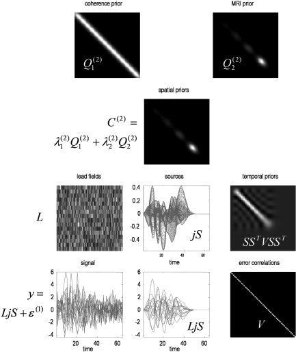
Simulated data. The spatial smoothness or coherence and MRI priors are shown in the top panels. These are prior covariance components, over sources, shown in image format. The smoothness component is stationary (i.e., does not change along the diagonals), whereas the fMRI prior changes with source location. The resulting spatial priors λ${}_{\text{1}}^{\text{(2)}}$Q${}_{\text{1}}^{\text{(2)}}$ + λ${}_{\text{2}}^{\text{(2)}}$Q${}_{\text{2}}^{\text{(2)}}$ are shown below. The temporal priors on the sources SS ^T VSS ^T are shown on the middle right. Again, these are depicted as a covariance matrix over time bins. Notice how this prior concentrates signal variance in the first forty time bins. Data (middle panel) were generated in source space, using random Gaussian variates according to the forward model in equation (10) and the spatial and temporal priors above. These were passed thought the lead‐field matrix to simulate channel data. In this example, the lead field matrix was simply a matrix of independent Gaussian variates. The lower left panels show the channel data after (left) and before (right) adding noise, over time bins.

ReML solution

The simulated channel data were used to estimate the covariance components and implicitly the spatial priors using equation (12). The resulting estimates of λ = [λ${}_{\text{1}}^{\text{(1)}}$, λ${}_{\text{1}}^{\text{(2)}}$, λ${}_{\text{2}}^{\text{(2)}}$] are shown in Figure 3(upper panel). The small bars represent 90% confidence intervals about the ReML estimates, based on the curvature of the log‐likelihood in equation (7). The large bars are the true values. The ReML scheme correctly assigns much more weight to the MRI priors to provide the empirical prior in the lower panel (left). This ReML estimate (left) is virtually indistinguishable from the true prior (right).

Figure 3.

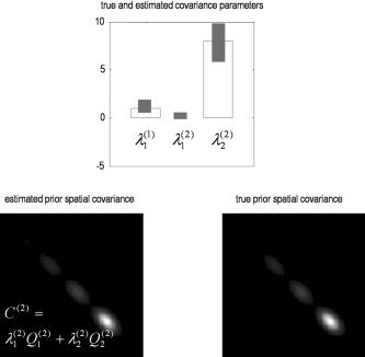
Restricted maximum likelihood (ReML) solution. The ReML estimates of λ = [λ${}_{\text{1}}^{\text{(1)}}$, λ${}_{\text{1}}^{\text{(2)}}$, λ${}_{\text{2}}^{\text{(2)}}$] are shown in the upper panel. The small bars represent 90% confidence intervals about the ReML estimates based on the curvature of the log likelihood. The large bars are the true values. The ReML scheme correctly assigns more weight to the MRI priors to provide the empirical prior in the lower panel (left). This ReML estimate is virtually indistinguishable from the true prior (right).

Conditional estimates of responses

The conditional expectations of sources, over time, are shown in Figure 4 using the expression in equation (13). The upper left panel shows the true and estimated spatial profile at the time‐bin expressing the largest activity (maximal deflection). The equivalent source estimate over time is shown on the right. One can see the characteristic shrinkage of the conditional estimators in relation to the true values. The full spatiotemporal profiles are shown in the lower panels.

Figure 4.

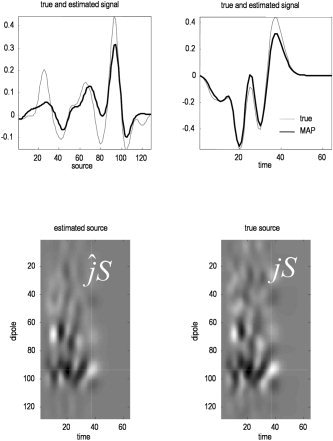
Conditional estimates of responses. The upper panel shows the true and estimated spatial profile at the time‐bin expressing the largest activity (upper left). The equivalent profile, over time, is shown on the upper right for the source expressing the greatest response. These graphs correspond to sections (dotted lines) though the full spatiotemporal profiles shown in image format (lower panels). Note the characteristic shrinkage of the maximum aposteriori (MAP) estimates relative to the true values that follows from the use of shrinkage priors (that shrink the conditional expectations to the prior mean of zero).

Conditional estimates of response energy

To illustrate the estimation of energy, we defined a time‐frequency window W = [w(t)sin(ωt), w(t)cos(ωt)] for one frequency, ω, over a Gaussian time window, w(t). This time‐frequency subspace is shown in the upper panels of Figure 5. The corresponding energy was estimated using equation (17) and is shown with the true values in the lower panels. The agreement is evident.

Figure 5.

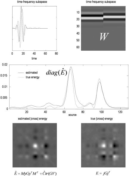
Conditional estimates of response energy. A time‐frequency subspace W is shown in the upper panels as functions of time (left) and in image format (right). This subspace defines the time‐frequency response of interest. In this example, we are testing for frequency‐specific responses between 10 and 20 time bins. The corresponding energy estimates are shown over sources with the true values in the middle panel. Note the remarkable correspondence. The lower panels show the cross‐energy over sources with estimates on the left and true values on the right. The energies in the middle panel are the leading diagonals of the cross‐energy matrices, shown as images below. Again note the formal similarly between the true and estimated cross‐energies.

Analysis of real data

We used MEG data from a single subject while they made symmetry judgments on faces and scrambled faces (for a detailed description of the paradigm see Henson et al. [2003]). MEG data were sampled at 625 Hz from a 151‐channel CTF Omega system (VSM MedTech, Coquitlam, Canada) at the Wellcome Trust Laboratory for MEG Studies, Aston University, England. The epochs (80 face trials, collapsing across familiar and unfamiliar faces, and 84 scrambled trials) were baseline‐corrected from −100 msec to 0 msec. The 500 msec after stimulus onset of each trial entered the analysis. A T1‐weighted MRI was also obtained with a resolution 1 × 1 × 1 mm³. Head‐shape was digitized with a 3D Polhemus Isotrak (Polhemus, Colchester, VT) and used to coregister the MRI and MEG data. A segmented cortical mesh was created using Anatomist (http://www.brainvisa.info//) [Mangin et al.,2004], with approximately 4,000 dipoles oriented normal to the gray matter. Finally, a single‐shell spherical head model was constructed using BrainStorm (http://neuroimage.usc.edu/brainstorm/) [Baillet et al.,2004] to compute the forward operator L.

The spatial covariance components comprised

(28)

where spatial smoothness operator D was defined on the cortical mesh using a Gaussian kernel with a standard deviation of 8 mm. We used only one, rather smooth spatial component in this analysis. This was for simplicity. A more thorough analysis would use multiple components and Bayesian model selection to choose the optimum number of components [Mattout et al., submitted]. As with the simulated data analysis, the noise correlations were assumed to be identical and independently distributed, V ⁽¹⁾ = I _t and the signal subspace in time S was specified by the first r = 50 principal eigenvectors of the windowed auto‐correlation matrix used above.

We focused our analysis on the earliest reliable difference between faces and scrambled faces, as characterized by the M170 component in the ERF (Fig. 6, middle panel). A frequency band of 10–15 Hz was chosen on the basis of reliable differences (P < 0.01; corrected) in a statistical parametric map (time‐frequency SPM) of the global energy differences (Fig. 6, upper right) around the M170 latency [Henson et al.,2005a]. The ensuing time‐frequency subspace was centered at 170 msec (Fig. 6; middle).

Figure 6.

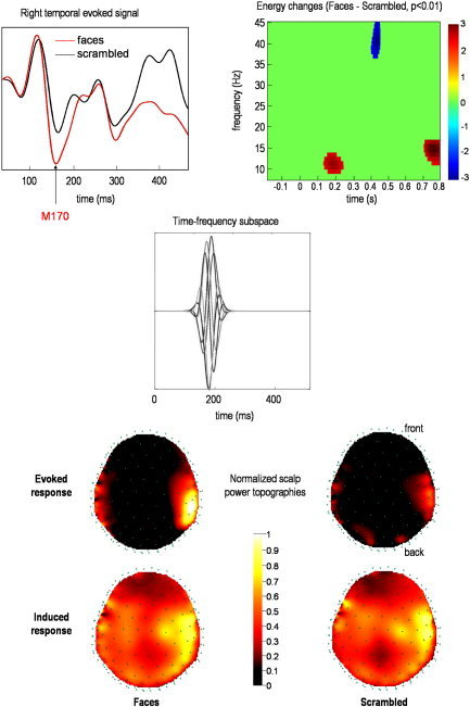
Real data analysis: sensor level. The upper panel shows the differences measured on the scalp between faces and scrambled faces, in terms of the event‐related field (ERF) from a single sensor (left), and the global energy over sensors (right) using standard time‐frequency analysis and statistical parametric mapping [Kilner et al.,2005]. The time‐frequency subspace W we tested is shown in the middle panel by plotting each column as a function of time. This uses the same representation as the first panel of the previous figure. This subspace tests for responses in the α range, around 200 msec (see corresponding time‐frequency effect in the upper right panel). The corresponding induced and evoked energy distributions over the scalp are shown in the lower panel for two conditions (faces and scrambled faces).

RESULTS

The lower panel of Figure 6 shows evoked and induced power in channel space as defined in equations (23) and (26) respectively. Power maps were normalized to the same maximum for display. In both conditions, maximum power is located over the right temporal regions; however, the range of power values is much wider for the evoked response. Moreover, whereas scalp topographies of induced responses are similar between conditions, the evoked energy is clearly higher for faces, relative to scrambled faces. This suggests that the M170 is mediated by differences in phase‐locked activity.

This is confirmed by the power analysis in source space (Fig. 7), using equations (23) and (26). Evoked and induced responses are generated by the same set of cortical regions. The differences between faces and scrambled faces in terms of induced power, however, are weak compared to the equivalent differences in evoked power (see the scale bars in Fig. 7). Furthermore, the variation in induced energy over channels and conditions is small relative to evoked power. This nonspecific profile suggests that ongoing activity may contribute substantially to the induced component. As mentioned above, the interesting aspect of induced power usually resides in trial‐specific differences. A full analysis of induced differences will be presented elsewhere. Here we focus on the functional anatomy implied by evoked differentials. The functional anatomy of evoked responses, in this context, is sufficiently well known to establish the face validity of our conditional estimators:

Figure 7.

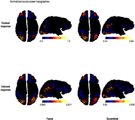
Real data analysis: source level. Reconstructed evoked and induced responses are shown for both faces and scrambled face trials. These data correspond to conditional expectations rendered onto a cortical surface. These views of the cortical surface are from below. (i.e., left is on the right). Evoked power was normalized to the maximum over cortical sources.

The upper panel of Figure 8 shows the cortical projection of the difference between the conditional expectations of evoked energy for faces versus scrambled faces. The largest changes were expressed in the right inferior occipital gyrus (IOG), the right orbitofrontal cortex (OFC), and the horizontal posterior segment of the right superior temporal sulcus (STS). Figure 9 shows the coregistration of these energy changes with the subject's structural MRI. Happily, the “activation” of these regions is consistent with the equivalent comparison of fMRI responses [Henson et al.,2003].

Figure 8.

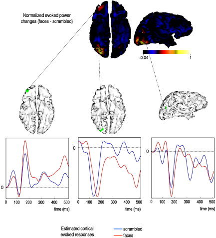
Real data analysis: evoked responses. The upper panel shows the reconstructed evoked power changes between faces and scrambled faces. The lower panel shows the reconstructed evoked responses associated with three regions where the greatest energy change was elicited.

Figure 9.

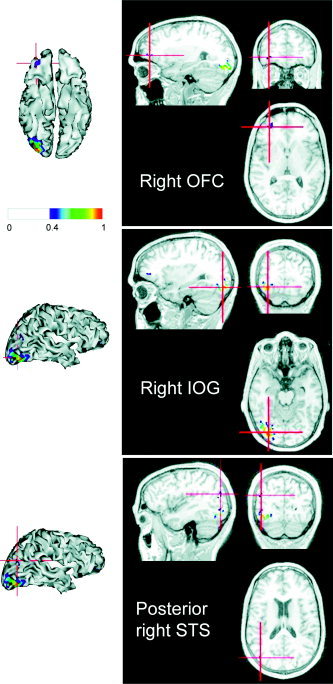
Visualization on the subject MRI. The regions identified as showing energy changes for faces versus scrambled faces in Figure 8 are shown coregistered with a MRI scan: the right orbitofrontal cortex (OFC; upper panel), the right inferior occipital gyrus (IOG; middle panel), and the posterior right superior temporal sulcus (STS; lower panel). These source estimates are shown both as cortical renderings (from below) and on orthogonal sections through a structural MRI, using the radiological convention (right is left).

The activation of the ventral and lateral occipitotemporal regions is also consistent with recent localizations of the evoked M170 [Henson et al.,2005b; Tanskanen et al.,2005]. This is to be expected given that the most of the energy change seems to be phase‐locked [Henson et al.,2005a]. Indeed, the conditional estimates of evoked responses at the location of the maximum of energy change in the right IOG and right posterior STS show a deflection around 170 msec that is greater for faces than scrambled faces (Fig. 8, lower panel).

We have not made any inferences about these effects. SPMs of energy differences would normally be constructed using conditional estimates of power changes over subjects. It is also possible, however, to use the conditional densities to compute a posterior probability map (PPM) of non‐zero changes for a single subject. We will demonstrate inference using these approaches elsewhere.

CONCLUSION

We have described an extension of our empirical Bayes approach to MEG/EEG source reconstruction that covers both evoked and induced responses. The estimation scheme is based on classical covariance component estimation using restricted maximum likelihood (ReML). We have extended the scheme using temporal basis functions to place constraints on the temporal form of the responses. We show how one can estimate evoked responses that are phase‐locked to the stimulus and induced responses that are not. This inherent distinction calls for different transformations of a hierarchical model of multiple trial responses to provide Bayesian estimates of power.

Oscillatory activity is well known to be related to neural coding and information processing in the brain [Fries et al.,2001; Hari and Salmelin,1997; Tallon‐Baudry et al.,1999]. Oscillatory activity refers to signals generated in a particular frequency band time‐locked but not necessarily phase‐locked to the stimulus. Classical data averaging approaches may not capture this activity, which calls for trial‐to‐trial analyses. Localizing the sources of oscillatory activity on a trial‐by‐trial basis is computationally demanding, however, and requires data with low signal‐to‐noise ratio. This is why early approaches were limited to channel space [e.g., Tallon‐Baudry et al.,1997]. Recently, several inverse algorithms have been proposed to estimate the sources of induced oscillations. Most are distributed (or imaging) methods, since equivalent current dipole models are not suitable for explaining a few hundreds of milliseconds of nonaveraged activity. Among distributed approaches, two main types can be distinguished: the beamformer [Cheyne et al.,2003; Gross et al.,2001; Sekihara et al.,2001] and minimum‐norm‐based techniques [David et al.,2002; Jensen and Vanni,2002], although both can be formulated as (weighted) minimum norm estimators [Hauk,2004]. A strict minimum norm solution obtains when no weighting matrix is involved [Hamalainen et al.,1993] but constraints such as fMRI‐derived priors have been shown to condition the inverse solution [Lin et al.,2004]. Beamformer approaches implement a constrained inverse using a set of spatial filters (see Huang et al. [2004] for an overview). The basic principle employed by beamformers is to estimate the activity at each putative source location while suppressing the contribution of other sources. This means that beamformers look explicitly for uncorrelated sources. Although some robustness has been reported in the context of partially correlated sources [Van Veen et al.,1997], this aspect of beamforming can be annoying when trying to characterize coherent or synchronized cortical sources [Gross et al.,2001].

Recently, we proposed a generalization of the weighted‐minimum norm approach based on hierarchical linear models and empirical Bayes, which can accommodate multiple priors in an optimal fashion [Phillips et al.,2005]. The approach involves a partitioning of the data covariance matrix into noise and prior source variance components, whose relative contributions are estimated using ReML. Each model (i.e., set of partitions or components) can be evaluated using Bayesian model selection [Mattout et al., submitted]. Moreover, the ReML scheme is computationally efficient, requiring only the inversion of small matrices. So far this approach has been limited to the analysis of evoked responses, because we have focused on the estimation of spatial covariance components under simple assumptions about the temporal correlations. In this article, we provided the operational equations and procedures for obtaining conditional estimates of responses with specific temporal constraints over multiple trials. The proposed scheme offers a general Bayesian framework that can incorporate all kind of spatial priors such as beamformer‐like spatial filters or fMRI‐derived constraints. Furthermore, basis functions enable both the use of computationally efficient ReML‐based variance component estimation and the definition of priors on the temporal form of the response. This implies a separation of the temporal and spatial dependencies both at the sensor and source levels using a Kronecker formulation [Huizenga et al.,2002]. Thanks to this spatiotemporal approximation, the estimation of induced responses from multitrial data does not require a computationally demanding trial‐by‐trial approach [Jensen and Vanni,2002] or drastic dimension reduction of the solution space [David et al.,2002].

The approach described in this article allows for spatiotemporal modeling of evoked and induced responses under the assumption that there is a subspace S in which temporal correlations among the data and signal have the same form. Clearly this subspace should encompass as much of the signal as possible. In this work, we used the principal eigenvariates of a prior covariance based on smooth signals concentrated early in peristimulus time. This subspace is therefore informed by prior assumptions about how and when signal is expressed. A key issue here is what would happen if the prior subspace did not coincide with the true signal subspace. In this instance there may be a loss of efficiency as experimental variance is lost to the null space of S; however, there will be no bias in the (projected) response estimates. Similarly, the estimate of the error covariance components will be unbiased but lose efficiency as high frequency noise components are lost in the restriction. Put simply, this means the variability in the covariance parameter estimates will increase, leading to a slight overconfidence in conditional inference. The overconfidence problem is not an issue here because we are only interested in the conditional expectations, which would normally be taken to a further (between‐subject) level for inference.

As proof of principle, we used a toy example and a single‐subject MEG data set to illustrate the methodology for single‐trial and multiple‐trial analyses, respectively. The toy data allowed us to detail how spatial and temporal priors are defined whereas the real data example provisionally addressed the face validity of the extended framework. In future applications, the priors will be considered in greater depth, such as fMRI‐derived constraints in the spatial domain and autoregressive models in the temporal domain. Importantly, SPM of the estimated power changes in a particular time‐frequency window, over conditions or over subjects, can be now achieved at the cortical level [Brookes et al., 2004; Kiebel and Friston,2004a]. Finally, with the appropriate wavelet transformation, instantaneous power and phase could also be estimated to study cortical synchrony.

REFERENCES

- Baillet S, Mosher JC, Leahy RM (2004): Electromagnetic brain imaging using brainstorm. Proceedings of the 2004 IEEE International Symposium on Biomedical Imaging (ISBI)., 15–18 April 2004, Arlington, VA.
- Brookes MJ, Gibson AM, Hall SD, Furlong PL, Barnes GR, Hillebrand A, Singh KD, Holliday IE, Francis ST, Morris PG (2005): A general linear model for MEG beam former imaging. Neuroimage 23: 936–946. [DOI] [PubMed] [Google Scholar]
- Cheyne D, Gaetz W, Garnero L, Lachaux J‐P, Ducorps A, Schwartz D, Varela FJ (2003): Neuromagnetic imaging of cortical oscillations accompanying tactile stimulation. Brain Res Cogn Brain Res 17: 599–611. [DOI] [PubMed] [Google Scholar]
- David O, Garnero L, Cosmelli D, Varela J (2002): Estimation of neural dynamics from MEG/EEG cortical current density maps: application to the reconstruction of large‐scale cortical synchrony. IEEE Trans Biomed Eng 49: 975–987. [DOI] [PubMed] [Google Scholar]
- Dietterich TG (2000): Ensemble methods in machine learning. Proceedings of the First International Workshop on Multiple Classifier Systems. London: Springer‐Verlag; p 1–15. [Google Scholar]
- Fries P, Reynolds JH, Rorie AE, Desimone R (2001): Modulation of oscillatory neuronal synchronization by selective visual attention. Science 291: 1506–1507. [DOI] [PubMed] [Google Scholar]
- Friston KJ (2000): The labile brain I. Neuronal transients and nonlinear coupling. Philos Trans R Soc Lond B Biol Sci 355: 215–236. [DOI] [PMC free article] [PubMed] [Google Scholar]
- Friston KJ, Penny W, Phillips C, Kiebel S, Hinton G, Ashburner J (2002): Classical and bayesian inference in neuroimaging: theory. Neuroimage 16: 465–483. [DOI] [PubMed] [Google Scholar]
- Gross J, Kujala J, Hamalainen M, Timmermann L, Schnitzler A, Salmelin R (2001): Dynamic imaging of coherent sources: studying neural interactions in the human brain. Proc Natl Acad Sci USA 98: 694–699. [DOI] [PMC free article] [PubMed] [Google Scholar]
- Hamalainen M, Hari R, Ilmoniemi R, Knuutila J, Lounasmaa O (1993): Magnetoencephalography: theory, instrumentation and applications to noninvasive study of human brain functions. Rev Mod Phys 65: 413–497. [Google Scholar]
- Hari R, Salmelin R (1997): Human cortical oscillations: a neuromagnetic view through the skull. Trends Neurosci 20: 44–49. [DOI] [PubMed] [Google Scholar]
- Hauk O (2004): Keep it simple: a case for using classical minimum norm estimation in the analysis of EEG and MEG data. Neuroimage 21: 1612–1621. [DOI] [PubMed] [Google Scholar]
- Henson RN, Goshen‐Gottstein Y, Ganel T, Otten LJ, Quayle A, Rugg MD (2003): Electrophysiological and haemodynamic correlates of face perception, recognition and priming. Cereb Cortex 13: 793–805. [DOI] [PubMed] [Google Scholar]
- Henson R, Kiebel S, Kilner J, Friston K, Hillebrand A, Barnes GR, Singh KD (2005a): Time‐frequency SPMs for MEG data on face perception: power changes and phase‐locking. Presented at the 11th Annual Meeting of the Organization for Human Brain Mapping, 12–16 June 2005, Toronto, Canada.
- Henson R, Mattout J, Friston K, Hassel S, Hillebrand A, Barnes GR, Singh KD (2005b): Distributed source localization of the M170 using multiple constraints. Presented at the 11th Annual Meeting of the Organization for Human Brain Mapping, 12–16 June 2005, Toronto, Canada.
- Huang M, Aine CJ, Supek S, Best E, Ranken D, Flynn ER (1998): Multi‐start downhill simplex method for spatio‐temporal source localization in magnetoencephalography. Electroencephalogr Clin Neurophysiol 108: 32–44. [DOI] [PubMed] [Google Scholar]
- Huang MX, Shih JJ, Lee DL, Harrington DL, Thoma RJ, Weisend MP, Hanlon F, Paulson KM, Li T, Martin K, Miller GA, Canive JM (2004): Commonalities and differences among vectorized beamformers in electromagnetic source imaging. Brain Topogr 16: 139–158. [DOI] [PubMed] [Google Scholar]
- Huizenga HM, de Munk JC, Waldorp LJ, Grasman RP (2002): Spatiotemporal EEG/MEG source analysis based on a parametric noise covariance model. IEEE Trans Biomed Eng 49: 533–539. [DOI] [PubMed] [Google Scholar]
- Jensen O, Vanni S (2002): A new method to identify sources of oscillatory activity from magnetoencephalographic data. Neuroimage 15: 568–574. [DOI] [PubMed] [Google Scholar]
- Kiebel SJ, Friston KJ (2004a): Statistical parametric mapping for event‐related potentials: I. Generic considerations. Neuroimage 22: 492–502. [DOI] [PubMed] [Google Scholar]
- Kiebel SJ, Friston KJ (2004b): Statistical parametric mapping for event‐related potentials: II. A hierarchical temporal model. Neuroimage 22: 503–520. [DOI] [PubMed] [Google Scholar]
- Kilner JM, Kiebel SJ, Friston KJ (2005): Applications of random field theory to electrophysiology. Neurosci Lett 374: 174–178. [DOI] [PubMed] [Google Scholar]
- Lin FH, Witzel T, Hamalainen MS, Dale AM, Belliveau JW, Stufflebeam SM (2004): Spectral spatiotemporal imaging of cortical oscillations and interactions in the human brain. Neuroimage 23: 582–595. [DOI] [PMC free article] [PubMed] [Google Scholar]
- Mangin JF, Riviere D, Cachia A, Duchesnay E, Cointepas Y, Papadopoulos‐Orfanos D, Scifo P, Ochiai T, Brunelle F, Regis J (2004): A framework to study the cortical folding patterns. Neuroimage 23: 129–138. [DOI] [PubMed] [Google Scholar]
- Mattout J, Phillips C, Rugg MD, Friston KJ. MEG source localisation under multiple constraints: an extended Bayesian framework. Neuroimage (submitted). [DOI] [PubMed]
- Phillips C, Mattout J, Rugg MD, Maquet P, Friston KJ (2005): An empirical Bayesian solution to the source reconstruction problem in EEG. Neuroimage 24: 997–1011. [DOI] [PubMed] [Google Scholar]
- Phillips C, Rugg MD, Friston KJ (2002): Anatomically informed basis functions for EEG source localization: combining functional and anatomical constraints. Neuroimage 16: 678–695. [DOI] [PubMed] [Google Scholar]
- Sekihara K, Nagarajan SS, Poeppel D, Marantz A, Miyashita Y (2001): Reconstructing spatio‐temporal activities of neural sources using an MEG vector beamformer technique. IEEE Trans Biomed Eng 48: 760–771. [DOI] [PubMed] [Google Scholar]
- Tallon‐Baudry C, Bertrand O, Delpuech C, Pernier J (1997): Oscillatory γ‐band (30–70Hz) activity induced by a visual search task in humans. J Neurosci 17: 722–734. [DOI] [PMC free article] [PubMed] [Google Scholar]
- Tallon‐Baudry C, Bertrand O (1999): Oscillatory gamma activity in humans and its role in object representation. Trends Cogn Sci 3: 151–162. [DOI] [PubMed] [Google Scholar]
- Tanskanen T, Nasanen R, Montez T, Paallysaho J, Hari R (2005): Face recognition and cortical responses show similar sensitivity to noise spatial frequency. Cereb Cortex 15: 526–534. [DOI] [PubMed] [Google Scholar]
- Trujillo‐Barreto NJ, Aubert‐Vazquez E, Valdes‐Sosa PA (2004): Bayesian model averaging in EEG/MEG imaging. Neuroimage 21: 1300–1319. [DOI] [PubMed] [Google Scholar]
- Van Veen BD, van Drongelen W, Yuchtman M, Suzuki A (1997): Localization of brain electrical activity via linearly constrained minimum variance spatial filtering. IEEE Trans Biomed Eng 44: 867–880. [DOI] [PubMed] [Google Scholar]