

Abstract
The ultimate goal of brain connectivity studies is to propose, test, modify, and compare certain directional brain pathways. Path analysis or structural equation modeling (SEM) is an ideal statistical method for such studies. In this work, we propose a two‐stage unified SEM plus GLM (General Linear Model) approach for the analysis of multisubject, multivariate functional magnetic resonance imaging (fMRI) time series data with subject‐level covariates. In Stage 1, we analyze the fMRI multivariate time series for each subject individually via a unified SEM model by combining longitudinal pathways represented by a multivariate autoregressive (MAR) model, and contemporaneous pathways represented by a conventional SEM. In Stage 2, the resulting subject‐level path coefficients are merged with subject‐level covariates such as gender, age, IQ, etc., to examine the impact of these covariates on effective connectivity via a GLM. Our approach is exemplified via the analysis of an fMRI visual attention experiment. Furthermore, the significant path network from the unified SEM analysis is compared to that from a conventional SEM analysis without incorporating the longitudinal information as well as that from a Dynamic Causal Modeling (DCM) approach. Hum. Brain Mapp, 2007. © 2006 Wiley‐Liss, Inc.
Keywords: dynamic causal modeling, fMRI, general linear model, multivariate autoregressive, structural equation modeling, subject‐level covariates, visual attention study
INTRODUCTION
During a typical functional MRI (fMRI) experiment, each subject's functional activity in the brain is measured longitudinally over the course of several minutes. In addition, data are acquired for multiple brain regions of interest (ROIs). Thus, for each subject one obtains multivariate time series data from the fMRI experiment. Furthermore, as with most biomedical studies, a group of subjects is usually evaluated in order to obtain meaningful estimation for the population of interest. Therefore, fMRI studies typically encompass multisubject, multivariate times series data. In addition, virtually all imaging studies involve subject‐level covariates such as age, gender, education, and measurements of motor, behavioral, and cognitive functions. It is essential to incorporate these “external measurements” or covariates into the analysis to determine the relationships between functional brain pathways and subjects' cognitive, behavioral, or motor function.
Path analysis, also referred to as structural equation modeling (SEM), was originally developed in the early 1970s by Jöreskog, Keesling, and Wiley, when they combined factor analysis with econometric simultaneous equation models [Jöreskog and Sorbom, 1996; see Bollen, 1989; Bollen and Long, 1993; Loehlin, 1998, for an overview]. In the early 1990s McIntosh introduced SEM to neuroimaging [McIntosh and Gonzales‐Lima, 1991, 1994a, b; McIntosh et al., 1994; McIntosh, 1998] for modeling, testing, and comparison of directional effective connectivity of the brain. SEM has quickly become popular in this field [Büchel and Friston, 1997, 1999; Bullmore et al., 1996, 2000; Fletcher et al., 1999; Glabus et al., 2003; Grafton et al., 1994; Honey et al., 2002; Jennings et al., 1998]. This tool is now available in commercial software packages including LISREL, EQS, AMOS, and SAS [Bentler, 1992, 1995; Bentler and Wu, 1993, 2002; Jöreskog and Sorbom, 1996].
However, no existing SEM software has the correct procedure for the analysis of fMRI data because the implemented procedures assume independent observations [Bentler and Wu, 2002; pers. commun. with authors of EQS and LISREL]. This assumption is not true for fMRI time series since the measured fMRI signals are temporally correlated. In other words, neither traditional SEM methods nor existing software packages for modeling the human brain connectivity can readily analyze such multisubject, multivariate time series data with subject‐level covariates.
The recently released SPM2 (Statistical Parametric Mapping software, http://www.fil.ion.ucl.ac.uk/spm) features the “dynamic causal modeling (DCM)” procedure for estimating the effective connectivity [Friston et al., 2003]. The goal of DCM is to construct a reasonably realistic neuronal model of interacting cortical regions. DCM is also called a dynamic input‐state‐output model in the sense that experimentally designed input stimuli modulate the state variables, which include neuronal activities and other neurophysiological or biophysical variables, to evoke the output variables [Friston et al., 2003; Penny et al., 2003]. DCM has been specifically designed for the analysis of functional imaging data, whereas SEM was developed for other areas of science. A major difference between DCM and SEM is that the paths of DCMs are estimated by the modulating effect of certain inputs on the neuronal states, while SEM paths are obtained by minimizing the discrepancy between observed and implied correlations/covariances of hemodynamically convolved BOLD signals (i.e., fMRI data). A comprehensive review of DCM and SEM can be found in Ramnani et al. [ 2004] and Stephan et al. [ 2004]. Despite their differences, both methods may still be improved in order to cope with the complex fMRI data structure and the sophisticated underlying neurobiological processes. The current DCM, for example, only permits the analysis of a small network with no more than eight brain regions due to algorithmic limitations. Additionally, neither method can model the temporal correlation of the observed fMRI data directly.
As an attempt to partially fill this void, we propose a two‐stage unified SEM/GLM (General Linear Model) approach for the analysis of multisubject, multivariate time series fMRI data with subject‐level covariates. In Stage 1, we analyze the fMRI multivariate time series data for each subject individually via a unified SEM approach. In Stage 2, the resulting subject‐level path coefficients are merged with subject‐level covariates such as gender, age, IQ, education, etc., to examine the impact of these covariates on brain pathways via a GLM. To address the validity of our modeling method, we compared the results of the proposed unified SEM approach with those of a conventional SEM analysis as well as a DCM analysis of an fMRI visual attention study.
Unified SEM Approach
As the first stage of the proposed two‐stage algorithm, we analyze the fMRI multivariate time series data for each subject individually via a “unified” SEM approach, which includes longitudinal as well as contemporaneous relations. Specifically, longitudinal temporal relations are defined as relationships between brain regions involving different time points, and are represented in the form of a multivariate autoregressive model (MAR). Conversely, contemporaneous relations reflect relationships between brain regions at the same time point, and involve conventional SEMs.
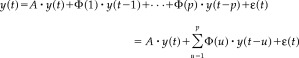
Let y j(t) be the j th variable (e.g., the average BOLD intensity for the j th ROI) measured at time t, j = 1, 2, …, m. The m‐dimensional multivariate autoregressive process of order p (MAR(p)) with an added component of contemporaneous relations can be written as:
 |
(1) |
Here y(t) = [y 1(t) y 2(t) … y m(t)]′ is the (m × 1) vector of observed variables measured at time t, ϵ(t) = [ϵ 1(t) ϵ2(t) … ϵm(t)]′ is an (m × 1) vector of white noise with zero‐mean and the error covariance θϵ, A is the parameter matrix of the contemporaneous relations, and Φ(i), i = 1, 2, …, p, is a series of (m × m) parameter matrices representing the longitudinal relations. The diagonal elements in the Φ(i)'s represent the coefficients of the autoregressive process for each variable, and the off‐diagonal elements represent the coefficients of the lagged relation between the variables. The parameter matrices A and Φ(i)'s may contain free, constrained, or fixed elements. These parameters are set by the initial path model with predefined paths. The details of this process will be illustrated through the fMRI visual attention example in the sections below.
Let Φ = [Φ(1) Φ(2) … Φ(p)] be a (m × (m × p)) parameter matrix and x = [y(t − 1) y(t − 2) … y(t − p)]′ be a (m × p) row vector. If we denote ϕ = {ϕi}as the set of free parameters of Φ, A, θϵ, and Λ the variance‐covariance structure of x, the implied covariance matrix of y(t) and x under model (1) is:
| (2) |
where B = (I − A)−1.
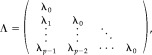
The variance‐covariance block matrix Λ of x = [y(t − 1) y(t − 2) … y(t − p)]′ in the model is:
 |
(3) |
where λi denotes a symmetric variance‐covariance matrix of the i‐lag cross‐covariances between y(t) = [y 1(t) y 2(t) … y m(t)]′ and y(t − i) = [y 1(t − i) y 2(t − i) … y m(t − i)]′. These lagged covariances λi's, i = 0, 1, …, p‐1, are calculated directly from the observed data. The rest of the free parameters in Σ(ϕ) are estimated by minimizing the discrepancy between the observed and the implied covariance structures of the variables.
Parameter Estimation
The set of unknown parameters, ϕ, is estimated so that the implied covariance matrix Σ(ϕ) is close enough to the sample covariance matrix S by minimizing the discrepancy or fitting functions F(S,Σ(ϕ)) [Browne, 1984, 1993]. There are three types of fitting functions: maximum likelihood (ML), unweighted least squares (ULS), and generalized least squares (GLS) functions. The most widely used fitting function for general structural equation models is the maximum likelihood function defined by:
| (4) |
where q is the number of variables in y and x.
Once the joint MAR‐SEM model is established as a unified SEM model, we can implement it using any traditional SEM package such as LISREL, EQS, or SAS. The unified SEM model is fitted to the fMRI time series for each individual subject and the model parameters are estimated thereafter. For the second‐stage GLM analysis, the estimated model parameters are treated as response variables, and their relations with the subject‐level covariates are examined via the GLM approach that can be easily implemented using standard statistical software such as SAS. In the following we illustrate this two‐stage approach via an fMRI visual attention study.
SUBJECTS AND METHODS
Subjects and Image Acquisition
Twenty‐eight volunteers (14 female and 14 male) who had no psychiatric or neurological disease history participated in this study. A visual attention experiment with a “three‐ball tracking” task (Fig. 1) [Lange, 1999; Kanwisher and Wojciulik, 2000; Jovicich et al., 2001] was conducted on a 4 T Varian (Palo Alto, CA) MR System at the Brookhaven National Laboratory (BNL) for each subject. The study was approved by the local Institutional Review Board and all subjects provided verbal and written consent.
Figure 1.
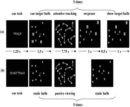
Schematic diagram of the visual stimulus used in (a) active tracking and (b) passive viewing trials. Each trial began with a text cue indicating the type of trial. This was followed by a period of static balls (1.5 s), in which the target balls were highlighted with orange squares on active trials. These highlights then disappeared and the balls moved in random directions about the screen without overlapping. After 7.75 s the balls stopped moving and were highlighted for 1 s only on active tracking trials, and subjects indicated (using a response button) whether the highlighted balls were among the balls that they had been tracking. Following this response, and after a delay of 0.5 s, the correct balls were re‐highlighted for 1 s to provide feedback to the subjects on the correctness of their response.
After a brief training session outside of the scanner, MRI was performed on a 4 T whole‐body scanner (Varian) using a quadrature headcoil. A single‐shot gradient‐echo EPI sequence (TE/TR = 25/3,000 ms, 4 mm slices, 1 mm gap, typically 33 coronal slices, 642 matrix, 20 cm field of view (FOV), 124 time points) was used to acquire fMRI time series. Task performance and subject motion were monitored online during fMRI [Caparelli et al., 2003] to assure accuracy >80%, motion <1 mm translations and <1° rotations.
Experimental Design
At the beginning of each trial subjects first saw a message for 1.25 s indicating whether their task would be active tracking (“TRACK”) or passive viewing (“DO NOT TRACK”). Next, 10 copper‐colored balls appeared at random positions on the screen, along with a central fixation cross. Subjects were asked to fixate throughout the entire trial. At the beginning of each active tracking trial, orange squares appeared for 1.5 s around three balls that the subject was asked to track; on passive‐viewing trials, the balls simply remained motionless for this 1.5‐s period. After this cue period the balls moved in random directions. When a ball approached another ball or the edge of the screen, it changed direction to avoid collision or overlap. After 7.75 s the balls stopped moving and three balls, chosen at random with equal likelihood to have been a target or nontarget, were highlighted for 1 s. Subjects lightly touched a button with their dominant hand (thumb) only if the balls were identical to those that they were tracking; their responses therefore provided an objective measure of tracking performance, with 50% being chance. The active tracking trial continued after a delay of 0.5 s, when the balls were highlighted again for 1 s for the next tracking session. The sequence of events was identical in the nontracking trials. However, no balls were highlighted, and the subjects were instructed not to track the balls but to view them passively.
Each active trial lasted for 60 s, comprising a total of five different active tracking modules within this period. Passive tracking trials also lasted for 60 s. The three‐ball tracking tasks consisted of three blocks of active tracking alternated with passive tracking.
Data Processing
Preprocessing of fMRI time series were performed in SPM99 (Statistical Parametric Mapping software, http://www.fil.ion.ucl.ac.uk/spm) and involved motion correction, spatial normalization to the Talairach frame, and spatial smoothing with an 8 mm FWHM Gaussian Kernel. Time series were bandpass‐filtered with the hemodynamic response function as a low‐pass filter and a high‐pass filter (cutoff frequency: 1/126 Hz). No slice timing correction was used. ROIs with a volume of (3 × 3 × 3) voxels were defined at the cluster center of each ROI to extract the average raw, unfiltered blood oxygenated level‐dependent (BOLD) time course using a customized program written in IDL.
We identified the following six regions, based on a literature review and the fact that they had strong activation during the ball‐tracking task: cerebellum (CEREB), posterior parietal cortex (PPC, BA 40), anterior parietal cortex (APC, BA 7), thalamus (THAL), medial frontal gyrus (MedFG, BA 8), and lateral prefrontal cortex (LPFC, BA 6, 9, 46) [Büchel and Friston, 1997; Chang et al., 2004; Corbetta et al., 1991; Friston and Büchel, 2000; Horwitz and Tagamets, 1999; Jovicich et al., 2001; Tagamets and Horwitz, 1998].
As described by Honey et al. [ 2002], the segments of each regional time series corresponding to presentation of the activation conditions were then extracted. To do so, we allowed a mean hemodynamic delay of 6 s (i.e., two TR periods) at the beginning of each onset condition. Therefore, the segments of signal corresponding to the presentation of each of the three activation conditions without the first two time points were concatenated as a set of task‐specific or within‐task time series (T = 54 time points) for each subject in each region [see Honey et al., 2002; Horwitz et al., 2000, for more details].
RESULTS
Stage 1: Analysis of the Unified SEM Model for the Visual Attention Study
In the previous section we discussed how to model the longitudinal and the contemporaneous components in the form of a joint MAR‐SEM model as a unified SEM. Here we exemplify this process through analysis of the visual attention data.
The initial path model is defined with six ROIs and seven anatomically possible directional paths for the left brain hemisphere. The starting region of visual attention processing in the model is the posterior parietal cortex (PPC), and information flows via the anterior parietal cortex (APC) to the lateral prefrontal cortex (LPFC). An attentional feedback loop starts at the medial frontal gyrus (MedFG), with input from the LPFC, and extends through the thalamus (THAL) back to the PPC. The THAL acts a subcortical “relay station,” and receives additional input from the cerebellum (CEREB) (Fig. 2). We restricted our model to the left hemisphere in order to simplify the brain network. This model is then defined as the theoretical contemporaneous path model for our experimental study. The longitudinal relations are depicted by the first‐order multivariate autoregressive process (MAR(1)). The order of MAR for each ROI obtained from the partial autocorrelation function (PACF) analysis was not always 1. However, due to estimability constraints [Honey et al., 2002], we chose the MAR of order 1 for all ROIs involved. While using the first‐order MAR process is proper in this study, for a new dataset one must examine its autocorrelation structure to determine which time series model is appropriate. The unified longitudinal and contemporaneous path model is then described via a path diagram in Figure 3, and the matrix form of the unified SEM with its contemporaneous and longitudinal components is outlined in Eq. 5. Specifically, Eq. 5 indicates that the value of one region at time (t) is influenced by other specified regions contemporarily as well as the value of the previous time (t‐1) of itself and of other specified regions.
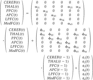 |
| (5) |
where y(t) = [CEREB(t) THAL(t) PPC(t) APC(t) LPFC(t)Med FG(t)] is a vector of the observed fMRI data of six brain regions at time t, A and Φ(l) are parameter matrices, and ε(t) = [ε 1(t) ε2(t) ε3(t) ε4(t) ε5(t) ε6(t)]′ is a vector of errors. The unified SEM model above with its contemporaneous SEM component of six ROIs and seven pathways, its MAR(1) longitudinal component and error variances, was fitted for each of the 28 subject time courses individually using the SAS PROC CALIS procedure. Table I presents the mean values of the estimated path coefficients with their standard errors across all 28 subjects. The t‐test statistic and the corresponding P‐value for each region in Table I provide the significant longitudinal and contemporaneous paths at the significance level of 0.05. The path model with the significant paths is displayed in Figure 4. The significant longitudinal path connections start at CEREB and connect the THAL, PPC, APC, and LPFC to MedFG as a single route of connectivity. The only significant contemporaneous path is from LPFC to MedFG. The same analysis was repeated using LISREL, with identical results as those from SAS.
Figure 2.
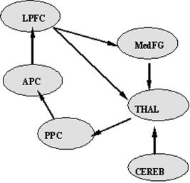
Path diagram of the theoretical contemporaneous path model with six ROIs; posterior parietal cortex (PPC), anterior parietal cortex (APC), lateral prefrontal cortex (LPFC), medial frontal gyrus (MedFG), thalamus (THAL), and cerebellum (CEREB), and seven directional pathways in the left hemisphere.
Figure 3.
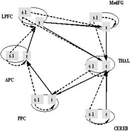
Unified longitudinal and contemporaneous path model. Six brain regions with 13 designed longitudinal paths (dashed lines) and 7 contemporaneous paths (solid lines) are described. The longitudinal connections are to one region at the current time (t) from other regions as well as itself at the past time (t‐1).
Table I.
Mean values of the estimated longitudinal and contemporaneous path parameters over 28 subjects with their standard errors, t test statistics, and corresponding P values (two‐sided)
| Longitudinal path parameters | Contemporaneous path parameters | ||||
|---|---|---|---|---|---|
| Path parameters | Mean (SE) | t value (P value) | Path parameters | Mean (SE) | t value (P value) |
| φ11 | 0.77 (0.09) | 8.67 (0.00) | α21 | 0.09 (0.07) | 1.23 (0.23) |
| φ21 | 0.46 (0.12) | 3.8 (0.00) | α25 | 0.10 (0.07) | 1.32 (0.20) |
| φ22 | −0.43 (0.20) | −2.16 (0.05) | α26 | 0.07 (0.08) | 0.85 (0.41) |
| φ25 | 0.19 (0.18) | 1.07 (0.31) | α32 | −0.04 (0.03) | −1.52 (0.14) |
| φ26 | 0.14 (0.17) | 0.85 (0.41) | α43 | −0.01 (0.04) | −0.16 (0.87) |
| φ32 | 0.57 (0.13) | 4.37 (0.00) | α54 | 0.09 (0.06) | 1.40 (0.17) |
| φ33 | 0.14 (0.07) | 2.15 (0.05) | α65 | 0.22 (0.06) | 3.97 (0.00) |
| φ43 | 0.55 (0.11) | 4.88 (0.00) | |||
| φ44 | 0.17 (0.10) | 1.67 (0.12) | |||
| φ54 | 0.58 (0.11) | 5.15 (0.00) | |||
| φ55 | −0.19 (0.15) | 1.26 (0.23) | |||
| φ65 | 0.53 (0.12) | 4.55 (0.00) | |||
| φ66 | −0.09 (0.15) | −0.62 (0.55) | |||
Bold characters indicate the significant path parameters at the significance level of 0.05.
Figure 4.
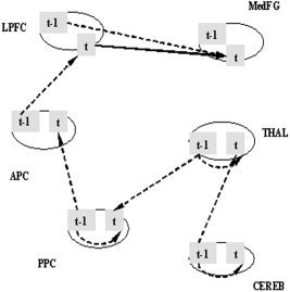
Significant path connections in the Stage 1 unified SEM model. The significant longitudinal path connections start at cerebellum (CEREB) and extend through thalamus (THAL), posterior parietal cortex (PPC), anterior parietal cortex (APC), and lateral prefrontal cortex (LPFC) to medial frontal gyrus (MedFG) in the left hemisphere. This path network contains one significant contemporaneous path from LPFC to MedFG.
Stage 2: Incorporating Subject‐Level Covariates via the GLM for the Visual Attention Study
In Stage 2 the subject‐level path coefficients obtained from the unified SEM analysis of Stage 1 are merged with the subject‐level covariate to examine the impact of these covariates on the brain pathways via a GLM. Here we illustrate the Stage 2 analysis using the same fMRI visual attention network study.
We examined the impact of four external covariates—gender, age, verbal IQ (VIQ), and education on the visual attention pathway. Four covariates of 28 subjects were fitted on a GLM for each path connection individually. The corresponding analysis results (F‐statistics and their P values) are tabulated in Table II. At the significance level of 0.05, four out of 13 longitudinal and 7 contemporaneous paths in this model were significantly influenced by gender, and two paths were influenced by age and VIQ (Fig. 5). However, no connectivity in this visual attention network was significantly correlated with education. In summary, gender is the most influential, while education has no impact on the unified SEM model.
Table II.
F‐test statistics and the corresponding P values (in parentheses) of four subject‐level covariates from the general linear model (GLM) analysis
| Paths | Gender | Age | VIQ | Education |
|---|---|---|---|---|
| φ11 | 0.01 (0.93) | 1.01 (0.33) | 0.15 (0.70) | 0.20 (0.66) |
| φ21 | 5.53 (0.03) | 5.56 (0.03) | 0.29 (0.60) | 0.11 (0.75) |
| φ22 | 4.63 (0.04) | 0.25 (0.62) | 1.79 (0.19) | 0.52 (0.48) |
| φ25 | 4.01 (0.06) | 0.23 (0.64) | 1.98 (0.17) | 0.42 (0.53) |
| φ26 | 2.24 (0.15) | 0.19 (0.67) | 0.05 (0.83) | 0.15 (0.70) |
| φ32 | 0.02 (0.90) | 0.02 (0.90) | 0.21 (0.65) | 0.26 (0.61) |
| φ33 | 0.12 (0.73) | 0.40 (0.53) | 0.40 (0.53) | 0.17 (0.68) |
| φ43 | 0.93 (0.35) | 0.58 (0.45) | 14.1 (0.00) | 0.07 (0.80) |
| φ44 | 0.24 (0.63) | 0.23 (0.64) | 0.13 (0.72) | 1.33 (0.26) |
| φ54 | 0.18 (0.68) | 0.04 (0.85) | 0.04 (0.85) | 0.24 (0.63) |
| φ55 | 0.89 (0.36) | 0.49 (0.49) | 1.16 (0.29) | 0.82 (0.38) |
| φ65 | 4.52(0.04) | 1.28 (0.27) | 2.81 (0.11) | 0.07 (0.80) |
| φ66 | 3.31 (0.08) | 2.19 (0.15) | 1.03 (0.32) | 0.42 (0.53) |
| α21 | 0.01 (0.94) | 0.35 (0.56) | 1.90 (0.18) | 0.01 (0.93) |
| α25 | 0.30 (0.59) | 0.01 (0.93) | 1.06 (0.31) | 0.33 (0.57) |
| α26 | 0.00 (0.97) | 2.36 (0.14) | 0.87 (0.36) | 1.92 (0.18) |
| α32 | 0.01 (0.91) | 1.86 (0.19) | 0.18 (0.68) | 0.10 (0.76) |
| α43 | 2.57 (0.12) | 0.06 (0.81) | 0.70 (0.41) | 0.62 (0.44) |
| α54 | 0.91 (0.35) | 7.70 (0.01) | 5.23 (0.03) | 0.02 (0.90) |
| α65 | 10.8 (0.00) | 0.02 (0.89) | 0.76 (0.39) | 1.21 (0.28) |
Bold characters indicate the paths significantly influenced by the corresponding covariates at the significance level of 0.05.
Figure 5.

This shows the paths which are significantly influenced by the corresponding subject variability from Table II. Three covariates (G, gender; A, age; and V, verbal IQ) are denoted along with the path connections.
Comparison with Conventional Path Analysis
We also examined the conventional SEM method for the same visual attention study by (wrongly) assuming that the fMRI observations are independent. The seven paths in conventional SEM are equal to the contemporaneous paths in the unified SEM (Fig. 2). This path model was fitted using the general SEM fitting method in LISREL to estimate the path parameters for each subject, and the averages of the estimated path coefficients over all 28 subjects are summarized in Table III. The small P values (<0.05) in Table III indicate significant path connections starting from THAL, passing through PPC, and concluding at APC. Therefore, the significant paths in the conventional SEM are a subset of the significant longitudinal connections in the unified SEM (Table I; Fig. 4).
Table III.
Mean values, standard errors (in parentheses), t test statistics and the corresponding P values (two‐sided; in parentheses) of the path parameters over the 28 subjects from the conventional SEM method
| Path connection | Mean (SE) | t value (P value) |
|---|---|---|
| CEREB → THAL | 0.23 (0.2) | 1.13 (0.26) |
| LPFC → THAL | −0.38 (0.21) | −1.79 (0.08) |
| MedFG → THAL | 0.56 (0.29) | 1.94 (0.06) |
| THAL → PPC | −0.24 (0.07) | −3.28 (0.00) |
| PPC →APC | 0.29 (0.08) | 3.5 (0.00) |
| APC →LPFC | −0.46 (0.24) | −1.89 (0.06) |
| LPFC → MedFG | −0.11 (0.1) | −1.1 (0.28) |
Bold characters indicate significant path parameters at the significance level of 0.05.
DCM Analysis and a Numerical Comparison to the Unified SEM Method
We performed the DCM analysis using the fMRI data from the visual attention (three‐ball tracking) study described above. In DCM, the neuronal states are modulated by designed exogenous effects indicated by driving connections, and the modulated states and designed modulatory connections change the values of intrinsic connections [Friston et al., 2003].
The initial DCM connectivity is identical to the initial contemporaneous path model defined in the previous SEM analysis (Fig. 2). We note here that we only considered intrinsic connections in the DCM model because they are interregional paths that are related to the directional connections in the unified SEM model. DCM and the unified SEM do not have identical path structure, in that DCM does not have explicit longitudinal and contemporaneous paths. In addition, DCM requires at least one driving or modulatory connection, while the regional time series used for the unified SEM approach was the active (or on‐set) condition data with no modulatory or task effect. Consequently, we added the sensory input “attention” to the posterior parietal cortex (PPC), indicating the active (or on‐set) condition. The sensory input is placed on the PPC because the attention paradigm is driven by input from the primary visual cortex, which has strong projections to the PPC. The initial path model was then fitted for each subject individually, and all parameters of the intrinsic and driving connections were estimated across 28 subjects [Friston et al., 2003; Penny et al., 2003]. The final model with the averaged path parameters and the percentage confidence that these values exceed a default threshold in SPM2, ln(2)/8 per s, is presented in Figure 6.
Figure 6.
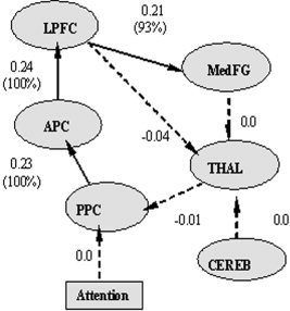
Estimated path coefficients averaged over 28 subjects from DCM analysis. Bold arrows indicate significant connections and dashed arrows indicate nonsignificant connections. The values in brackets reflect the percentage of confidence that these coefficients exceed a threshold of ln(2)/8 per s.
The significant DCM path network was found to be a subset of the significant unified SEM network, with three paths from PPC to MedFG through APC and LPFC. Two significant paths, from CEREB to THAL and then from THAL to PPC in the unified SEM, were no longer significant in the DCM analysis, possibly due to the addition of the sensory input.
DISCUSSION
In this work we propose a two‐stage approach, the unified SEM/GLM method, for the analysis of effective brain connectivity. This method enables the unified structural equation modeling of multisubject, multivariate time‐series fMRI data with subject‐level covariates. Specifically, this is done by modeling the longitudinal and the contemporaneous relations in the same SEM, analyzing this unified SEM for each subject separately, and then merging the resulting individual path parameters with other subject‐level covariates such as gender, age, IQ, education, etc., for the final GLM analysis to examine the influence of these covariates on the path model.
Historically, Harrison et al. [ 2003] were the first to introduce MAR into brain pathway analyses to characterize interregional dependence. Subsequently, Goebel et al. [ 2003] and Roebroeck et al. [ 2005] generalized the MAR approach by incorporating Granger causality maps between two time series. A comprehensive summary can be found in Stephan et al. [ 2004]. However, all of these methods represent an MAR approach. The unique feature of our new approach is that it is a unified SEM approach by incorporating directed contemporaneous and longitudinal relations in the same SEM model. Furthermore, the unified SEM models can be readily analyzed using any standard SEM software such as LISREL, EQS, and SAS. Although our method and those of Goebel et al. [ 2003] and Roebroeck et al. [ 2005] will lead to the same conclusion for studies with only two time series (i.e., two ROIs), the proposed approach is able to model an entire network with more than two regions. Additionally, we further incorporated the GLM to examine the impact of subject‐level covariates on the unified SEM pathways.
Also noteworthy is the dynamic factor analysis approach proposed by Molenaar [ 1985] and Molenaar et al. [ 1992], which was summarized in Hershberger et al. [ 1996]. Their work was motivated by the traditional psychological research work where the time trajectory is usually short and, therefore, their models deal with the case where the observed short time series trajectory can be explained by a latent factor series. In addition, they assume a fixed covariance structure (identity matrix) for the latent factor series to obtain an identified system. One might say, however, they are kindred spirits in the sense that had they been exposed to the problem of “path analysis of the fMRI time series data” that we encountered, they would have, very likely, generalized their method to the same “unified SEM” approach as we have.
This unified SEM/GLM approach is illustrated through the analysis of an fMRI visual attention study. Our analysis revealed the following longitudinal path connection CEREB → THAL → PPC → APC → LPFC → MedFG as a single route of connectivity. The only significant contemporaneous path is from LPFC to MedFG. Although prior studies indicated that the lateral geniculate nucleus is the early gatekeeper in the processing of visual information that is modulated by attention, and intermediate cortical‐processing areas, such as V4 and TEO, might be involved in filtering out unwanted information by means of receptive field mechanisms [Kastner and Pinsk, 2004], this longitudinal path illustrates the important role of the cerebellum in initiating the higher‐order cortical top‐down attention processing and feedback to the visual system. Surprisingly, the thalamus appears to be a relating site rather than a site of coordination in this model. Perhaps higher‐resolution fMRI techniques would reveal finer interconnections. Furthermore, more interconnections may be found if both hemispheres were modeled together.
We next examined the relationship between path connections and subject covariates by means of a GLM analysis. We found that gender is the most significant factor among four external covariates (age, gender, VIQ, and education) affecting four contemporaneous or longitudinal paths. In contrast, the education level had no influence on any path connection.
We also compared the unified SEM to the conventional SEM, omitting the temporal correlations. The conventional SEM analysis revealed only two significant pathways, from THAL to PPC and then to APC, which is a subset of the significant longitudinal pathways of the unified SEM approach. This suggests that omitting the temporal correlation within and between fMRI time‐series can have a significant impact on the resulting path models.
Finally, the DCM approach, which is widely available as part of the SPM package, was compared to the unified SEM approach using the same visual attention study. The unified SEM and the DCM approaches are in good agreement, and share all the significant pathways except those from CEREB to THAL and from THAL to PPC. It is likely that the driving connectivity from the task effect to the PPC has diminished these connections from the DCM analysis. Additional studies are necessary to further explore, compare, and possibly combine and improve these approaches.
Our study has certain technical limitations. First, fMRI data were acquired at a repetition time (TR) of 3 s, which may be considered long for effective modeling with DCM. Second, it is possible that the extracted time series used for the analysis may have been contaminated by aliasing of unwanted physiological signals, such as the cardiac cycle or respiration. Finally, the number of fMRI time points used for the unified SEM analyses was somewhat limiting in terms of modeling the entire network with both contemporaneous and longitudinal pathways. Future studies should take the sample size issue into consideration at the experimental design stage and generate sufficiently long time series.
REFERENCES
- Bentler PM (1992): EQS structural equation program manual. Cork, Ireland: BMDP Statistical Software. [Google Scholar]
- Bentler PM (1995): EQS structural equations program manual. Encino, CA: Multivariate Software. [Google Scholar]
- Bentler PM, Wu EJC (1993): EQS/Windows user's guide, v. 4 Cork, Ireland: BMDP Statistical Software. [Google Scholar]
- Bentler PM, Wu EJC (2002): EQS6 for Windows user's guide. Encino, CA: Multivariate Software. [Google Scholar]
- Bollen KA (1989): Structural Equations With Latent Variables. New York: John Wiley & Sons. [Google Scholar]
- Bollen KA, Long JS (1993): Testing Structural Equation Models. Thousand Oaks, CA: Sage. [Google Scholar]
- Browne MW (1984): Asymptotic distribution free methods in analysis of covariance structures. Br J Math Stat Psychol 37: 62–83. [DOI] [PubMed] [Google Scholar]
- Browne MW, Cudeck R (1993): Alternative ways of assessing model fit In: Bollen KA, Long JS, editors. Testing Structural Equation Models, vol. 154 Thousand Oaks, CA: Sage. [Google Scholar]
- Büchel C, Friston KJ (1997): Modulation of connectivity in visual pathways by attention: cortical interactions evaluated with structural equation modeling and fMRI. Cereb Cortex 7: 768–778. [DOI] [PubMed] [Google Scholar]
- Büchel C, Coull JT, Friston KJ (1999): The predictive value of changes in effective connectivity for human learning. Science 283: 1538–1541. [DOI] [PubMed] [Google Scholar]
- Bullmore ET, Rabe‐Hesketh S, Morris RG, Williams SCR, Gregory L, Gray JA, Brammer MJ (1996): Functional magnetic resonance image analysis of a large‐scale neurocognitive network. Neuroimage 4: 16–33. [DOI] [PubMed] [Google Scholar]
- Bullmore ET, Horwitz B, Honey G, Brammer M, Williams S, Sharma T (2000): How good is good enough in path analysis of fMRI data? Neuroimage 11: 289–301. [DOI] [PubMed] [Google Scholar]
- Caparelli E, Tomasi D, Arnold S, Chang L, Ernst T (2003): k‐Space based motion detection for functional MRI. Neuroimage 20: 1411–1418. [DOI] [PubMed] [Google Scholar]
- Chang L, Tomasi D, Yakupov R, Lozar C, Arnold S, Caparelli EC, Ernst T (2004): Adaptation of the attention network in human immunodeficiency virus brain injury. Ann Neurol 56: 259–272. [DOI] [PubMed] [Google Scholar]
- Corbetta M, Miezin FM, Dobmeyer S, Shulman GL, Petersen SE (1991): Selective and divided attention during visual discriminations of shape, color, and speed: functional anatomy by positron emission tomography. J Neurosci 11: 2383–2302. [DOI] [PMC free article] [PubMed] [Google Scholar]
- Fletcher P, Büchel C, Josephs O, Friston KJ, Dolan R (1999): Learning‐related neuronal responses in prefrontal cortex studied with functional neuroimaging. Cereb Cortex 9: 168–178. [DOI] [PubMed] [Google Scholar]
- Friston KJ, Büchel C (2000): Attentional modulation of effective connectivity from V2 to V5/MT in humans. Proc Natl Acad Sci U S A 97: 7591–7596. [DOI] [PMC free article] [PubMed] [Google Scholar]
- Friston KJ, Harrison L, Penny W (2003): Dynamic causal modeling. Neuroimage 19: 1273–1302. [DOI] [PubMed] [Google Scholar]
- Glabus MF, Horwitz B, Holt JL, Kohn PD, Gerton BK, Callicott JH, Lindenberg MA, Berman KF (2003): Interindividual differences in functional interactions among prefrontal, parietal and parahippocampal regions during working memory. Cereb Cortex 13: 1352–1361. [DOI] [PubMed] [Google Scholar]
- Goebel R, Roebroeck A, Kim DS, Formisano E (2003): Investigating directed cortical interactions in time‐resolved fMRI data using vector autoregressive modeling and Granger causality mapping. Magn Reson Imaging 21: 1251–1261. [DOI] [PubMed] [Google Scholar]
- Grafton ST, Sutton J, Couldwell W, Lew M, Waters C (1994): Network analysis of motor system connectivity in Parkinson's disease: modulation of thalamocortical interactions after pallidotomy. Hum Brain Mapp 2: 45–55. [Google Scholar]
- Harrison L, Penny WD, Friston KJ (2003): Multivariate autoregressive modeling of fMRI time series. Neuroimage 19: 1477–1491. [DOI] [PubMed] [Google Scholar]
- Hershberger SL, Molenaar PCM, Corneal SE (1996): A hierarchy of univariate and multivariate structural time series models In: Marcoulides GA, Schumacker RE, editors. Advanced Structural Equation Modeling: Issues and Techniques. Mahwah, NJ: Lawrence Erlbaum; p 159–194. [Google Scholar]
- Honey GD, Fu CHY, Kim J, Brammer MJ (2002): Effects of verbal working memory load on corticocortical connectivity modeled by path analysis of functional magnetic resonance imaging data. Neuroimage 17: 573–582. [PubMed] [Google Scholar]
- Horwitz B, Tagamets M‐A (1999): Predicting human functional maps with neural net modeling. Hum Brain Mapp 8: 137–142. [DOI] [PMC free article] [PubMed] [Google Scholar]
- Horwitz B, Friston KJ, Taylor JG (2000): Neural modeling and functional brain imaging: An overview. Neural Netw 13: 829–846. [DOI] [PubMed] [Google Scholar]
- Jennings JM, McIntosh AR, Kapur S (1998): Mapping neural interactivity onto regional activity: an analysis of semantic processing and response mode interactions. Neuroimage 7: 244–254. [DOI] [PubMed] [Google Scholar]
- Jöreskog KG, Sorbom D (1996): LISREL 8. User's reference guide. Chicago: Scientific Software International. [Google Scholar]
- Jovicich J, Peters RJ, Christofkoc H, Braun J, Chang L, Ernst T (2001): Brain areas specific for attentional load in a motion‐tracking task. J Cogn Neurosci 13: 1048–1058. [DOI] [PubMed] [Google Scholar]
- Kanwisher N, Wojciulik E (2000): Visual attention: insights from brain imaging. Nat Rev Neurosci 1: 91–100. [DOI] [PubMed] [Google Scholar]
- Kastner S, Pinsk MA (2004): Visual attention as a multilevel selection process. Cogn Affect Behav Neurosci 4: 483–500. [DOI] [PubMed] [Google Scholar]
- Lange N (1999): Statistical procedures for functional MRI In: Moonen C, Bandettini PA, editors. Functional MRI (Medical Radiology/Diagnostic Imaging). New York: Springer Medicine; 27:301–335. [Google Scholar]
- Loehlin JC (1998): Latent Variable Models: An Introduction to Factor, Path, and Structural Analysis, 4th ed. Mahwah, NJ: Lawrence Erlbaum. [Google Scholar]
- McIntosh AR (1998): Understanding neural interactions in learning and memory using function neuroimaging. Ann N Y Acad Sci 855: 556–571. [DOI] [PubMed] [Google Scholar]
- McIntosh AR, Gonzales‐Lima F (1991): Structural modeling of functional neural pathways mapped with 2‐deoxyglucose; effects of acoustic startle habituation on the auditory system 7. Brain Res 547: 295–302. [DOI] [PubMed] [Google Scholar]
- McIntosh AR, Gonzales‐Lima F (1994a): Structural equation modeling and its application to network analysis in functional brain imaging. Hum Brain Mapp 2: 2–22. [Google Scholar]
- McIntosh AR, Gonzales‐Lima F (1994b): Network interactions among limbic cortices, basal forebrain, and cerebellum differentiate a tone conditioned as a Pavlovian excitor or inhibitor: fluorodeoxyglucose mapping and covariance structural modeling. J Neurophysiol 72: 1717–1733. [DOI] [PubMed] [Google Scholar]
- McIntosh AR, Grady CL, Haxby JV, Underleider LG, Horwitz B (1994): Network analysis of cortical visual pathways mapped with PET. J Neurosci 14: 655–666. [DOI] [PMC free article] [PubMed] [Google Scholar]
- Molenaar PCM (1985): A dynamic factor model for the analysis of multivariate time series. Psychometrika 50: 181–202. [Google Scholar]
- Molenaar PCM., de Gooijer JG, Schmitz B (1992): Dynamic factor analysis of nonstationary multivariate time series. Psychometrika 57: 333–349. [Google Scholar]
- Penny WD, Stephan KE, Mechelli A, Friston KJ (2003): Comparing dynamic causal models. Neuroimage 22: 1157–1172. [DOI] [PubMed] [Google Scholar]
- Ramnani N, Behrens T, Penny WD, Matthews PM (2004): New approaches for exploring anatomical and functional connectivity in the human brain. Biol Psychiatry 56: 613–619. [DOI] [PubMed] [Google Scholar]
- Roebroeck A, Formisano E, Goebel R (2005): Mapping directed influence over the brain using Granger causality and fMRI. Neuroimage 25: 230–242. [DOI] [PubMed] [Google Scholar]
- Stephan KE, Harrison LM, Penny WD, Friston KJ (2004): Biophysical models of fMRI response. Curr Opin Neurobiol 14: 629–635. [DOI] [PubMed] [Google Scholar]
- Tagamets M‐A, Horwitz B (1998): Integrating electrophysiological and anatomical experimental data to create a large‐scale model that simulates a delayed match‐to‐sample human brain imaging study. Cereb Cortex 8: 310–320. [DOI] [PubMed] [Google Scholar]