Segmentation of skull and scalp in 3‐D human MRI using mathematical morphology

Abstract

We present a new technique for segmentation of skull and scalp in T₁‐weighted magnetic resonance images (MRIs) of the human head. Our method uses mathematical morphological operations to generate realistic models of the skull, scalp, and brain that are suitable for electroencephalography (EEG) and magnetoencephalography (MEG) source modeling. We first segment the brain using our Brain Surface Extractor algorithm; using this, we can ensure that the brain does not intersect our skull segmentation. We next generate a scalp mask using a combination of thresholding and mathematical morphology. We use the scalp mask in our skull segmentation procedure, as it allows us to automatically exclude background voxels with intensities similar to those of the skull. We find the inner and outer skull boundaries using thresholding and morphological operations. Finally, we mask the results with the scalp and brain volumes to ensure closed and nonintersecting skull boundaries. Visual evaluation indicated accurate segmentations of the cranium at a gross anatomical level (other than small holes in the zygomatic bone in eight subjects) in all 44 MRI volumes processed when run using default settings. In a quantitative comparison with coregistered CT images as a gold standard, MRI skull segmentation accuracy, as measured using the Dice coefficient, was found to be similar to that which would be obtained using CT imagery with a registration error of 2–3 mm. Hum Brain Mapp, 2005. © 2005 Wiley‐Liss, Inc.

INTRODUCTION

Solutions to magnetoencephalography (MEG) and electroencephalography (EEG) inverse problems require realistic models of the head for use in accurate computation of the mapping from neural current sources to scalp potentials and extracranial magnetic fields [Mosher et al., 1999]. Since the conductivity of skull is significantly lower than that of soft tissue, it is crucial that bone regions be included in the head model [Hamalainen and Sarvas, 1989; Oostendorp and van Oosterom, 1989]. Because of the existence of closed form solutions for the MEG and EEG forward problem, multilayer spherical models have traditionally been used to approximate the human head with a set of nested spheres representing brain, skull, and scalp [Ary et al., 1981; Sarvas, 1987; Zhang, 1995]. Recently, representations of the head as a set of contiguous regions bounded by surface tessellations of the scalp, outer skull, inner skull, and brain boundaries have been used to provide more realistic models [Hamalainen and Sarvas, 1989; Schlitt et al., 1995]. Using boundary element methods in conjunction with these models produces more accurate results than the multilayer spherical model but requires that a volumetric image of the subject's head first be segmented into its component bone and soft tissue regions.

CT and MRI serve different functions in biomedical imaging. CT exhibits better bone definition than is seen with MRI; however, it does not provide good contrast in soft tissue. In addition, CT is not a preferred modality for routine anatomical imaging of structures in the head because of the exposure of the subject to ionizing radiation. Conversely, MRI does an excellent job of differentiating soft tissues, including cerebral cortex and blood vessels, but it does not provide accurate detail of bone structures, such as the skull, because of the weak magnetic resonance signals produced in bone. Segmentation of skull from MRI thus presents a challenging problem. The development of methods for segmenting skull and scalp from MRI enables the production of patient‐specific models of scalp, skull, and brain from a single, high‐resolution MRI of the complete head.

RELATED WORK

Although numerous MRI segmentation techniques are described in the literature, there is little research dedicated to the problem of segmenting skull in MRI, as CT has typically been used for this purpose. Classification of skull in MRI has often been a by‐product of classification techniques designed to categorize brain tissue. Held et al. [1997] used a Markov random field (MRF) approach to classify MRI data into gray matter, white matter, cerebrospinal fluid (CSF), scalp‐bone, and background. This method does not guarantee continuous bounding contours, and it was not developed for the purpose of segmentation of the skull in MRI. Chu and Takaya [1993] detected the skin–skull and skull–brain boundaries using thresholding and Laplacian of Gaussian (LoG) operations on successive transverse slices. Congorto et al. [1996] and Belardinelli et al. [2003] used neural networks‐based approaches to segment skull and brain also from successive T₁ MRI slices. Another technique was introduced by Heinonen et al. [1997], who used thresholding and region growing to segment bone in MRI volumes. Haque et al. [1998] also used simple thresholding and manual segmentation to detect the boundaries of skull and scalp to create an average head model for forward modeling in MEG. Performing the segmentation on individual slices does not allow the method to exploit the connected 3‐D structure of the skull. With thresholding and region growing methods, the segmentation of certain bone regions, such as ocular globes, is difficult because of partial volume effects. Rifai et al. [1999] applied a deformable model to segment skull from MRI. Deformable models can be attracted to incorrect boundaries resulting in the potential inclusion of skin, muscles, eyes, and inner ear in the segmented skull.

Techniques have also been developed that make use of information from multiple modalities. Studholme et al. [1996] used CT information for segmentation of skull in coregistered MRI of the same subject. Soltanian‐Zadeh and Windham [1997] applied a multiscale approach where they made use of both CT and MRI information. The choice of an approach that requires both CT and MRI, while attractive in providing accurate detail of both skull and soft tissue, is not generally practical since acquisition using both modalities is rarely performed in either volunteer or clinical studies. Wolters et al. [2002] note that the inner skull boundary can be determined more accurately in proton density (PD) than in T₁‐weighted MRI since the CSF produces a stronger signal than skull in the former case, while the two are barely distinguishable in the latter. Using coregistered PD and T₁‐weighted images, they produce a segmentation based on adaptive fuzzy c‐means clustering and extended region growing [Wolters, 2003]. For solving the forward problem in EEG these results are then extended to include anisotropy in conductivity in the skull using diffusion tensor imaging to estimate the conductivity tensor [Haueisen et al., 2002]. The forward problem is then solved using a finite element method. Akahn et al. [2001] also use PD and T₁ images to segment skull, scalp, CSF, eyes, and white and gray matter with a hybrid algorithm that uses snakes, region growing, morphological operations, and thresholding. While these approaches are attractive, and the use of PD images will lead to improved segmentation of skull, in the vast majority of brain imaging studies only high‐resolution T₁‐weighted images are collected. Consequently, there is a need for a robust approach to segmentation of skull and scalp from T₁‐weighted images only.

There are a limited number of software packages that offer skull segmentation from T₁‐weighted MRI. These include Brain Extraction Tool (BET) produced by Smith et al. [2001], ANATOMIC produced by Heinonen et al. [1998], and BRain Image ANalysis (BRIAN) produced by Kruggel and Lohmann [1996]. In BET, the brain is first segmented from the MRI and then the outer skull boundary is found by searching outwards from the brain surface and determining the maximum gradient in intensity combined with an ad hoc thresholding procedure. In ANATOMIC, the skull is segmented using thresholding and region growing as described above. Other software packages, such as ANALYZE and CURRY, can also be used to segment skull and scalp in T₁‐weighted MRI. However, the segmentation procedures are not automatic. These methods require a user‐defined sequence of thresholding and application of included morphological tools to obtain the skull and scalp boundaries.

Most previous studies have not provided quantitative validation of methods for segmenting skull in MRI. Instead, many relied on the analysis of physicians to qualitatively approve their results. However, skull is not a very apparent structure in T₁‐weighted MRI, and even for trained clinical experts the determination of the boundaries of the skull within this modality is difficult.

Here we describe our approach to this problem, which we base on a sequence of thresholding and morphological operations. We also present a quantitative validation study of our method, which uses coregistered MRI‐CT data to evaluate our results.

OBTAINING ANATOMICAL SURFACES WITH MORPHOLOGICAL PROCESSING

Accurate segmentation of skull in MRI is difficult because the magnetic resonance signal from bone is weak and often indistinguishable from air; it is further complicated by the topology of the skull. Certain parts of the skull, such as the ocular globes and portions of the upper region of the skull, are thin compared to the resolution currently available in MRI. This problem is confounded by partial volume effects that tend to reduce the apparent thickness of the skull. In regions in which bone and air are separated by thin layers of tissue (e.g., sinuses, external auditory canals) it is often difficult to differentiate between air and bone voxels [Rifai et al., 1999].

Binary mathematical morphology is an algebraic system based on set theory that provides two basic operations: dilation and erosion. Combinations of these operations enable underlying object shapes to be identified and reconstructed from their noisy distorted forms. A combination of dilation and erosion gives rise to two additional operations, opening and closing, which form the basis for most morphological processing [Nadadur and Haralick, 2000]. Morphological approaches have already been widely used in segmentation of magnetic resonance imagery [Bomans et al., 1990; Brummer et al., 1993; Shattuck et al., 2001].

Our method performs skull and scalp segmentation using a sequence of morphological operations. We first segment the brain using our Brain Surface Extractor (BSE) [Sandor and Leahy, 1997; Shattuck et al., 2001; Shattuck and Leahy, 2002]. We exclude the brain from the image volume to obtain an estimate of the intensity distribution of the scalp and the skull regions. From this, we compute a threshold that we use to perform an initial segmentation of the scalp, which we refine with mathematical morphology. When we segment the skull we use the scalp segmentation to distinguish between dark voxels that may be skull or air, since these areas will have overlapping intensity distributions and may appear connected through the sinuses. We also use the brain mask to ensure that our skull boundary does not intersect the brain boundary. Figure 1 provides a complete block diagram of our algorithm for segmenting scalp and skull using morphological operations.

Figure 1.

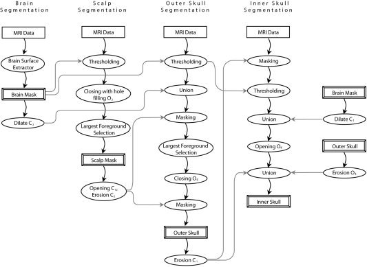
Block diagram of our algorithm for scalp and skull segmentation using morphological operations. On completion, we apply additional masking operations to ensure that scalp, outer skull, inner skull, and brain masks do not intersect each other.

Mathematical Morphology

Morphological operators use a binary image and a structuring element as input and combine them using intersection, union, inclusion, or complement operators. We use three basic structuring elements: the cube, the 3‐D cross, and the 3‐D octagon. These elements are shown in Figure 2, along with their corresponding 2‐D structuring elements. The 3‐D octagon, which we denote by O ₂, is an approximation of a sphere and is defined as the dilation of the 3‐D cross by the 3‐D cube. This is analogous to an octagon shape in 2‐D, which is produced by the dilation of a 3 × 3 square by a 3 × 3 cross.

Figure 2.

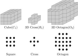
Basic structuring elements used in our algorithm: Cube (C ₁), 3‐D Cross (R ₁), 3‐D Octagon (O ₂), and their corresponding 2‐D structuring elements: Square, Cross, and Octagon.

Dilation or erosion by larger structuring elements is performed by applying the operation multiple times with a smaller structuring element. For instance, if we want to apply a dilation operation using C ₄, a cubic structuring element of radius 4, to some object S, we can achieve this by applying dilation 4 times using C ₁, a cube of radius 1:

(1)

We use the following mathematical symbols for the morphological operators in the description of our algorithm: ⊕ for dilation, ⊖ for erosion, ○ for opening, • for closing, and ⊙ for a special form of closing operation with hole filling, described in detail below.

Segmentation of Brain

We segment the brain using BSE software, v. 3.0 [Sandor and Leahy, 1997; Shattuck et al., 2001; Shattuck and Leahy, 2002]. BSE identifies the brain using anisotropic diffusion filtering, Marr‐Hildreth edge detection, and morphological operations. Preprocessing with an anisotropic diffusion filter improves the edge definitions in the MRI by smoothing nonessential gradients in the volume without blurring steep edges. The Marr‐Hildreth edge detector identifies important anatomical boundaries such as the boundary between brain and skull. The brain is identified and refined using a sequence of morphological and connected component operations. The output of BSE is a binary mask, denoting brain and nonbrain.

Skull and Scalp Thresholds

We compute initial segmentations for the skull and scalp using thresholding with values computed from the image after brain extraction. The voxels that are not labeled as brain are typically either low intensity regions (the background, some parts of CSF and skull) or higher intensity regions (fat, skin, muscle, and other soft tissues). We compute an empirical skull threshold as the mean of the intensities of the nonzero voxels that are not brain. We define this set as:

(2)

where V is a set of spatial indices referencing the entire MRI volume, B is a set of voxels identified by BSE as brain, V\B is the set of voxels in V excluding B, and m _k is the k‐th voxel in the MRI volume. The threshold is then:

(3)

where m _j is the intensity of the j ^th voxel in V, the MRI, and X _NB is the set of nonzero and nonbrain voxels.

The scalp surface is the interface between the head and the background in the image. Its transition is quite sharp, thus our primary concern is to find an appropriate threshold that removes noise in the background. We compute the scalp threshold as the mean of the nonbrain voxels that are at or above t _skull:

(4)

where m _j is the intensity of the j ^th voxel in V, and X _NS is defined as:

(5)

These thresholds give the algorithm an initial estimate of the range of the skull and scalp intensities. In our implementation of the algorithm, these thresholds may also be adjusted by the user to improve the segmentation.

Scalp Segmentation

Thresholding the MRI with t _scalp produces a set of foreground voxels described by:

(6)

where t _scalp is the scalp threshold and x _k is the k ^th voxel value (see Fig. 3b). After thresholding, the volume will still contain background voxels that result from noise. It will also have cavities in the head that correspond to regions of tissue that have low‐intensity values such as CSF. These cavities will often be connected to the background through the sinuses or auditory canals. To address these problems, we apply a modified morphological closing operation. A traditional closing operation consists of a dilation followed by an erosion, both of which use the same structuring element. Our closing operation, which we denote by ⊙, performs a hole‐filling operation between dilation and erosion; this will fill any cavities that are disjoint from the background after dilation. We obtain the scalp volume by applying our modified closing operation to X _{t_scalp}, the thresholded volume, using a structuring element O ₂ (see Fig. 3c–e):

(7)

Figure 3.

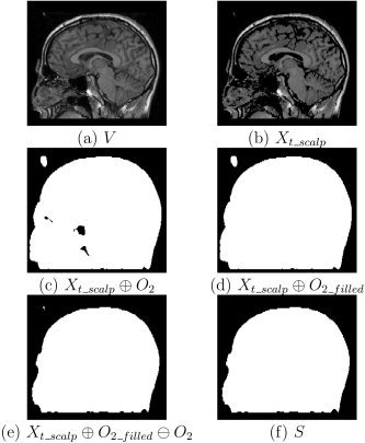
Different stages of scalp segmentation: (a) slice in the initial MRI volume; (b) image after applying a threshold, X _{t_scalp}; (c) dilated image; (d) image with cavities filled; (e) eroded image; (f) largest foreground component.

Since the connection of auditory canals and sinuses to the outside environment is through ears and nose, application of the dilation operator with an O ₂ structuring element closes these structures. A subsequent hole‐filling closing operation produces a single volume that contains the entire head, including brain and skull as well as scalp. We then select the largest foreground connected component as the head volume:

(8)

where SCC is an operator that selects the largest foreground connected component in the set X _{t_scalp_filled}. The set S differentiates scalp from background. Figure 3 shows views of each stage of the scalp identification process.

Segmentation of Skull

Finding the skull in T₁‐weighted MRI is difficult because the skull appears as a set of dark voxels and typically has a thickness of only three or four voxels. To properly segment the skull, we must identify both the outer boundary, which separates it from the scalp, and the inner boundary, which encases the brain.

Segmentation of outer skull.

Our outer skull segmentation procedure first performs a thresholding operation to identify the dark voxels in the image. As described above, we estimate the threshold for skull, t _skull, as the mean intensity value of the nonzero voxels in the MRI volume that are not identified as brain. Application of this threshold to the image produces the set:

(9)

where once again V is a spatial index set representing the entire MRI volume and x _k is the k ^th voxel value in the MRI (see Fig. 4b).

Figure 4.

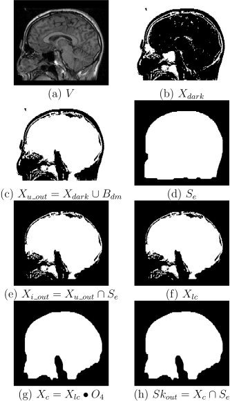
Outer skull segmentation. Stages of outer skull segmentation: (a) a slice in the MRI volume; (b) thresholding voxels with intensity less than or equal t _skull to identify the “dark” voxels (represented as white pixels in the image); (c) union of dark voxels and dilated brain mask; (d) modified scalp mask; (e) intersection of modified scalp mask and X _{u_out}; (f) largest connected component X _lc; (g) closed skull component; (h) final outer skull mask after masking by modified scalp mask.

The region identified by the thresholding operation will exclude some regions such as CSF that are inside the head but do not belong inside the skull. To capture these regions, we take the union of our thresholded image, X _dark, with a dilated brain mask, B _dm. We dilate the brain mask produced by BSE; we use a cube of radius 2, denoted as C ₂ (equivalent to a 5 × 5 × 5 cube), as the structuring element. This process, the result of which is shown in Figure 4c, is described as:

(10)

(11)

Next, we take the intersection of this volume with a modified scalp volume, S _e, to include only the dark voxels that lie within the head. We obtain this modified mask by applying an opening operation with cubic structuring element of radius 12 (25 × 25 × 25), followed by an erosion operation with a cube of radius 2 (5 × 5 × 5):

(12)

These two operations generate a scalp volume that typically does not include the ears or nose (see Fig. 4d). In particular, this volume excludes portions of the ear canals and nasal sinuses that have intensity values that are indistinguishable from skull. By masking the skull with S _e (see Fig. 4e), we ensure that these regions do not appear incorrectly as part of the skull and that the skull does not intersect the scalp boundary. This is described by:

(13)

where S _e is the modified scalp, and X _{i_out} is the initial skull mask.

The largest connected region resulting from this operation will be the closed volume bounded by the outer skull, but X _{i_out} may contain additional connected components such as the eyes. Thus, we now select the largest connected component in X _{i_out} to disconnect this volume from background voxels and eye sockets (see Fig. 4f):

(14)

We then close the boundary of the outer skull using a closing operation with the structuring element O ₄:

(15)

This closing operation may cause the volume to intersect the scalp, so our final operation is again to mask the volume with the eroded scalp to enforce the physical constraint that the outer skull boundary lies within the scalp volume that we previously computed:

(16)

The resulting set Sk _out is a closed volume bounded by the outer skull boundary (see Fig. 4h).

Segmentation of inner skull

Segmenting the inner boundary of the skull is more difficult than identifying the scalp or the outer skull. We must be careful to keep all parts of the brain and the CSF within the inner skull boundary. In some MRI volumes with low signal/noise ration (SNR), skull is difficult to distinguish from CSF, and CSF may therefore be misinterpreted as skull. In order to overcome this problem we use the outer skull and brain masks to restrict the allowed locations of the inner skull boundary.

First, we mask the MRI volume using a skull mask, Sk _{out_e}. We create Sk _{out_e} by eroding the outer skull set computed in the previous section, Sk _out, with a structuring element C ₁:

(17)

(18)

This ensures that the resultant inner skull will lie inside the outer skull. Then, we apply the same threshold t _skull we used to find the outer skull to the voxels in X _o:

(19)

The resulting volume should represent the region bounded by the inner skull boundary (see Fig. 5c). The thresholding operation produces holes in the volume resulting from CSF voxels that have intensities similar to that of the skull. Therefore, we take the union of the X _bright with a dilated brain mask to directly fill these nonskull regions (see Fig. 5d). We use the structuring element C ₁ to dilate the brain. With this operation we ensure that the mask X _{u_in} encloses the brain mask:

(20)

(21)

Figure 5.

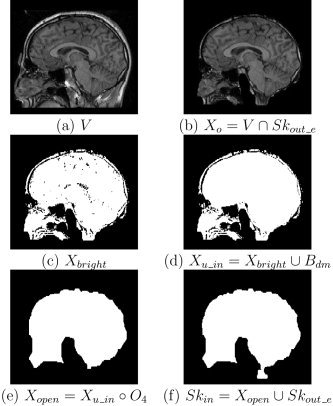
Inner skull segmentation. Stages of inner skull segmentation: (a) slice in the initial MRI volume; (b) image after masking by eroded outer skull mask; (c) binary image produced by thresholding X _o with t _skull; (d) image after union with dilated brain mask; (e) opening of X _{u_in} with O ₄; (f) inner skull mask produced from the union of X _open and the eroded outer skull.

The mask still appears noisy due to various remaining confounding features, such as bright voxels that correspond to diploic fat within the skull. We remove these regions by applying an opening operation using a structuring element O ₄ (see Fig. 5e):

(22)

While the previous steps will remove most CSF regions from the estimated skull mask, there may be regions where the dilated brain mask alone does not encompass all CSF, which therefore appears as part of the skull. To overcome this problem we impose a physical constraint on skull thickness in our algorithm and ensure that it does not exceed 4 mm. Using the structuring element O ₄, we apply an erosion operation to the outer skull volume. This produces the minimum interior skull boundary, Sk _{out_}:

(23)

By computing the union of Sk _{out_o} with X _open:

(24)

we obtain an inner skull boundary that better matches the anatomy (see Fig. 5f). Sk _in contains all voxels contained within the skull, but does not include the skull itself. While this operation will lead to underestimation of skull thickness in subjects with skulls thicker than 4 mm in places, it is a practical solution to the problem that CSF and skull are often indistinguishable. This thickness constraint can also be modified by the user. Because of partial volume effects and the resolution of the MRI data, the skull can be very thin in some parts of the image. This may cause problems in our segmentations because the resultant surface tessellations of the scalp, outer skull, inner skull, and brain boundaries may intersect. We therefore constrain our segmentation results to ensure that each structure does not intersect with the neighboring surfaces. To avoid affecting the brain segmentation result, we apply this constraint to the inner skull first, then to the outer skull, and finally to the scalp. We dilate the brain mask with structuring element C ₁ and take the union of this mask with the inner skull. We repeat the same procedure for the outer skull and scalp. We constrain the outer skull by taking its union with the dilated inner skull; we constrain the scalp by taking its union with the outer skull dilated with structuring element C ₁. This correction procedure guarantees that we obtain nonintersecting boundaries. Figure 6 gives a summary of our algorithm with the notation used in the equations. Figure 7 shows views of surface models generated from this procedure. The final set of masks differentiate brain, the space between brain and skull, skull, scalp, and background.

Figure 6.

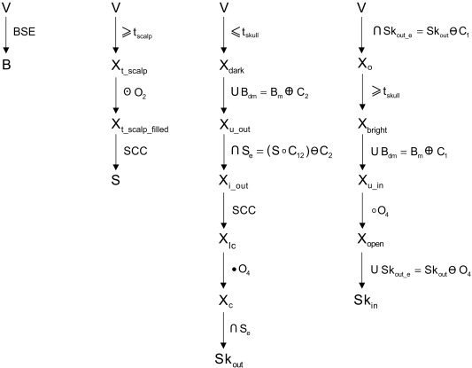
A more detailed block diagram of our algorithm for scalp and skull segmentation using morphological operations with the notations used in the equations. On completion, we apply additional masking operations to ensure that scalp, outer skull, inner skull, and brain masks do not intersect each other.

Figure 7.

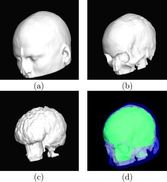
Renderings of surface tessellations of the head models: (a) scalp model; (b) outer skull model; (c) inner skull model; (d) nested view of the surfaces.

RESULTS

We performed two studies of the performance of our scalp and skull segmentation methods, which we implemented using the C++ programming language. In the first study we assessed the ability of our method to perform automatically on several MRI volumes. In the second study we measured the accuracy of our methods using coregistered sets of CT and MRI data.

Automation Study

We applied our algorithm to 44 T₁‐weighted MRI volumes obtained from the International Consortium for Brain Mapping (ICBM) Subject Database [Mazziotta et al., 2000]. Scalp segmentation was successful for all subjects with no manual intervention. For 36 of the 44 volumes our algorithm produced closed anatomically correct skull models with no user interaction. For the remaining eight volumes our algorithm also generated anatomically correct skull models that contained one or two holes near the eye sockets in the zygomatic bones. Of these, three were corrected by manually adjusting the skull threshold. In the other cases, adjusting the threshold to close the holes resulted in errors elsewhere in the skull. This problem arises because of the very thin bone layer in the vicinity of the zygomatic bone. However, these holes do not introduce additional openings in the cranium between the brain and scalp and so should have minimal impact on MEG and EEG fields calculated using these surfaces.

Coregistered CT/MRI Validation

We examined segmentation results from pairs of CT and T₁‐weighted MRI data volumes acquired from eight subjects. The CT‐MRI datasets were provided as part of the project “Retrospective Image Registration Evaluation” [West et al., 1997]. In this database, the T₁‐weighted MRI data were obtained using a Magnetization Prepared RApid Gradient Echo (MP‐RAGE) sequence. This is a rapid gradient‐echo technique in which a preparation pulse (or pulses) is applied before the acquisition sequence to enhance contrast [Mugler and Brookeman, 1990]. The dimensions of the MRI volumes were 256 × 256 × 128 with resolution on the order of 1 × 1 × 1.5 mm. The corresponding CT scans had 3 mm slice thickness with slice dimensions 512 × 512, with resolution on the order of 0.4 × 0.4 mm. The number of slices for each CT volume varied between 42 and 49.

We processed the CT and MRI data by registering each CT volume to its corresponding MRI volume. We used the 3‐D Multi‐Modal Image Registration Viewer Software (RView 8.0w Beta) to perform these registrations [Studholme et al., 1999]. After alignment, we used thresholding to label the skull in the CT datasets. We then used closing and flood filling procedures to fill the diploic spaces within the skull. We also labeled the scalp and brain in CT datasets using morphological operations. In this study we treated the segmentation results that we obtained from CT as a gold standard against which to compare the MRI segmentations. Figure 8 shows results of the segmentation of brain, skull, and scalp from a T₁‐weighted MRI volume and its corresponding CT data for transaxial, sagittal, and coronal sections. Figure 9 shows the results as tessellations of the scalp, outer skull, inner skull, and brain for four of the eight MRI datasets. Surface tessellations were computed using the Marching Cubes algorithm [Lorensen and Cline, 1987] and rendered using our BrainSuite software [Shattuck and Leahy, 2002].

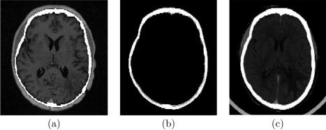
Figure 8.

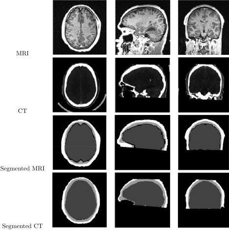
Segmentation of brain, CSF, skull, and scalp from MRI and its corresponding CT on transaxial, sagittal, and coronal slices respectively. First Row: Original MRI. Second Row: Original CT data. Third Row: Segmentation of brain, CSF, skull, and scalp from MRI. Fourth Row: Segmentation of combined brain/CSF, skull, and scalp from CT.

Figure 9.

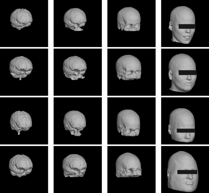
Surface tessellations of the brain, inner skull, outer skull, and scalp obtained from four MRI datasets

To assess the performance of our algorithm, we computed Dice coefficients between correspondingly labeled regions generated from the CT and MRI data. The Dice coefficient measures the similarity of two sets; it ranges from 0 for sets that are disjoint to 1 for sets that are identical. This metric is a special case of the kappa index that is used for comparing set similarity [Zijdenbos et al., 1994]. It is defined as:

(25)

where S ₁ and S ₂ are the two sets being compared.

Skull morphology in the lower portion of the head is extremely complex and performance of our algorithm in these regions is unreliable. However, forward modeling calculations in MEG and EEG are primarily affected by the scalp and the skull boundaries in the regions between the brain surface and the location of the scalp electrodes or external magnetometers. Consequently, we restricted our evaluation to the head volume lying above the plane passing through nasion and inion and perpendicular to the sagittal plane. While small portions of the occipital and temporal lobes may extend below this plane, and hence are excluded from the evaluation, the use of an anatomically defined bounding plane makes this analysis objective and repeatable and preferable to one in which the evaluation region is redefined for each subject.

For each subject we computed Dice coefficients measuring the similarity in segmentations of four regions that were labeled in the coregistered CT and MRI. These regions were the brain and CSF volume within the inner skull boundary, the skull (the region between the outer and the inner skull boundary), the region between the outer scalp boundary and the outer skull, and the whole head volume contained within the scalp. These results are listed in Table I. On average, the segmentations showed agreement metrics of 0.9436 ± 0.013 for brain/csf, 0.7504 ± 0.056 for skull, 0.7229 ± 0.061 for the region bounded by scalp and skull, and 0.9670 ± 0.013 for the scalp. Figure 10 shows an overlay of the MRI and CT skulls on transaxial MRI and CT sections for one of the datasets, illustrating the agreement of the two segmentations.

Table I.

Dice coefficients comparing the CSF and brain volume inside the skull, skull volume (i.e., the region between inner and outer skull boundaries), the region between outer skull and scalp boundary, and the whole head for 8 coregistered CT and MRI data sets

Subject no.	Brain/CSF	Skull	Region between scalp and outer skull	Scalp volume (whole head)
1	0.9452	0.7608	0.6820	0.9814
2	0.9472	0.7134	0.7665	0.9786
3	0.9540	0.6364	0.6123	0.9818
4	0.9189	0.7940	0.7228	0.9550
5	0.9451	0.7852	0.7752	0.9729
6	0.9315	0.7912	0.7488	0.9588
7	0.9517	0.7254	0.7924	0.9483
8	0.9553	0.7964	0.6832	0.9590
Average	0.9436 ± 0.013	0.7504 ± 0.056	0.7229 ± 0.061	0.9670 ± 0.013

CSF, cerebrospinal fluid; CT, computed tomography; MRI, magnetic resonance imaging.

Figure 10.

Overlay of the MRI and CT skulls on a transaxial MRI cross‐section and its corresponding coregistered CT cross‐section. a: Overlay of the MRI skull on MRI; white region corresponds to skull. b: Overlay of MRI and CT skulls. White voxels are labeled as skull in both CT and MRI segmentations; dark gray voxels are labeled as skull only in the MRI data; light gray voxels are labeled as skull only in the CT data; and black voxels are labeled as background in both. c: Overlay of the CT skull on coregistered CT.

The use of CT models for skull and scalp in EEG or MEG source localization would require registration of the CT data to MEG or EEG sensor positions, which typically has an accuracy on the order of 2.5 mm [de Munck et al., 2001; Lamm et al., 2001]. Consequently, it is worthwhile to relate the error induced by use of the skull segmentation from MRI with that which would result from registration error even if CT images were available. We thus compare the Dice coefficients presented in Table I for skull segmentation with Dice coefficients computed from misregistered copies of the CT skull model and the MRI skull model relative to the original CT skull model. We also compute a set difference measure:

(26)

which produces a value of 0 when all members of S _A are in S _B, and a value of 1 when no members of S _B are in S _A.

We shifted the CT skull volume by 1 mm, 2 mm, and 3 mm separately along each of the three cardinal axes in turn. We then computed the Dice coefficients and set differences between the shifted CT skulls and the original CT skull and the shifted CT skulls and MRI skull along each axis in turn. To compute the final results we calculated the average of the directional Dice coefficients and set differences to compute the results for 1 mm, 2 mm, and 3 mm shifts. Table II lists the average Dice coefficients and average set differences for the shifted CT skull relative to itself and to the MRI skull.

Table II.

Average Dice coefficients and average set differences for the comparison of 1 mm, 2 mm, and 3 mm misregistered CT skulls with itself and MRI skull

S1 vs. S2	Avg Dice Coef.	Avg diff(S1,S2)	Avg diff(S2,S1)
MRI vs. CT	0.7504 ± 0.0560	0.1658 ± 0.0727	0.3067 ± 0.0888
CT vs. CT1mm	0.9086 ± 0.0281	0.0925 ± 0.0280	0.0903 ± 0.0282
CT vs. CT2mm	0.8206 ± 0.0538	0.1819 ± 0.0540	0.1769 ± 0.0538
CT vs. CT3mm	0.7349 ± 0.0769	0.2679 ± 0.0767	0.2613 ± 0.0767
MRI vs. CT1mm	0.7346 ± 0.0599	0.1876 ± 0.0727	0.3220 ± 0.0863
MRI vs. CT2mm	0.6918 ± 0.0703	0.2337 ± 0.0775	0.3636 ± 0.0865
MRI vs. CT3mm	0.6337 ± 0.0858	0.3002 ± 0.0905	0.4158 ± 0.0955

CT, computed tomography; MRI, magnetic resonance imaging; Avg, average; coef., coefficient; diff, difference.

The Dice coefficients show that the errors between MRI and CT skull segmentations are similar to the effect of a 2–3 mm registration error. This figure is consistent with errors reported in the literature [de Munck et al., 2001; Lamm et al., 2001]. However, registration error will be present when using either CT or MRI, so a more realistic comparison is between the MRI and CT skull shifted by 2–3 mm and the corresponding CT and shifted CT skull. The MRI/shifted‐CT dice coefficients average 0.69 for a 2‐mm shift and 0.63 for a 3‐mm shift. In comparison, the CT/shifted‐CT dice coefficients average 0.82 for a 2‐mm shift and 0.73 for a 3‐mm shift. The set differences reported in Table II indicate that the lower dice coefficients for MRI/CT than CT/CT result from differences in the skull thickness in MRI and CT.

The set difference is asymmetric, and Table II shows that diff(MRI,CT) is less than diff(CT,MRI) for each case. This indicates that the CT skull is, on average, thicker than the MRI skull. This may be due to the absence of significant MRI signal from skull so that partial volume effects from the scalp tend to reduce the apparent skull thickness. Conversely, partial volume effects in CT, in which the skull has high intensity, may result in an overestimate of skull thickness. In the data used here this effect may be exacerbated by the 3‐mm slice thickness in the CT data, which will further tend to result in increased apparent skull thickness.

DISCUSSION AND CONCLUSIONS

We have developed a new algorithm for generating skull and scalp models from T₁‐weighted MRI. We tested our algorithm on 44 MRI datasets and performed additional quantitative validation using eight CT/MRI coregistered datasets. In both experiments we obtained anatomically accurate scalp and skull regions in a very short time. To assess the accuracy of our algorithm we computed Dice coefficients as a measure of the similarity of the segmentation results we obtained from coregistered CT and MRI datasets. We performed these comparisons on the upper portion of the head by defining a plane that is perpendicular to sagittal planes and passes through the nasion and the inion. We obtained an average Dice coefficient of 0.7504 ± 0.056 for the skull segmentation, 0.7229 ± 0.061 for the scalp segmentation, and 0.9670 ± 0.013 for the whole head. Comparison of these results with the effect of shifting the CT skull with respect to itself and the MRI skull indicate that the differences between the MRI and CT skulls are comparable to that which would arise from a registration error on the order of 2–3 mm. When the additional effect of 2–3 mm misregistration is added to the MRI/CT skull comparison, the Dice coefficients drop to a value equivalent to a registration‐only error in excess of 3 mm. The set difference measures also reported in Table II indicate that these results are due in large part to differences in skull thickness between CT and MRI. It is reasonable to conclude that this is caused in part by underestimation of skull thickness due to partial volume effects in the MRI. However, partial volume errors in the CT skull itself, as well as the skull thickening effects of the 3‐mm CT slices and additional registration errors arising from the CT/MRI registration, also contribute to the decrease in the MRI/CT Dice coefficients, while not adversely affecting the CT/CT values. Consequently, taking CT as the gold standard, the values reported in Table II represent a worse‐case performance and the effect of using an MRI‐segmented skull in place of one extracted from CT would be comparable to a registration error in excess of 3 mm. However, with the additional sources of error outlined here, we might expect effective performance with the MRI skull to be better than this. Furthermore, the skull thickness can be easily adjusted by changing the skull and scalp thresholds from the default values used in this study. In this case, more accurate skull volumes may be extracted. Since the primary application we envision for this skull segmentation method is in generating forward models for MEG and EEG, the impact of errors in definition of the skull layer should ultimately be assessed in terms of their impact on source localization accuracy; however, that is beyond the scope of this article.

As discussed above, in some instances one may adjust the skull and scalp thresholds to improve estimates of the skull volumes. The thresholds can be quickly adjusted, and identification of the scalp and skull surfaces on a 256 × 256 × 124 volume using the method described here requires less than 4 s of processing time on a 3 GHz Pentium IV processor. Our algorithm is integrated into our BrainSuite environment [Shattuck and Leahy, 2002], which is available online (http://brainsuite.usc.edu/).

REFERENCES

- Akahn Z, Acar CE, Gencer NG (2001): Development of realistic head models for electromagnetic source imaging of the human brain. Proc 23rd Annu EMBS Int Conf IEEE 1: 899–902.
- Ary JP, Klein SA, Fender DH (1981): Location of sources of evoked scalp potentials: corrections for skull and scalp thickness. IEEE Trans Biomed Eng BME 28: 447–452. [DOI] [PubMed] [Google Scholar]
- Belardinelli P, Mastacchi A, Pizzella V, Romani GL (2003): Applying a visual segmentation algorithm to brain structures MR images. Proc 1st Int IEEE EMBS Conf Neural Eng 507–510.
- Bomans M, Hohne K, Tiene U, Riemer M (1990): 3‐D segmentation of MR images of the head for 3‐D display. IEEE Trans Med Imaging 9: 177–183. [DOI] [PubMed] [Google Scholar]
- Brummer ME, Merseau RM, Eisner RL, Lewine RJ (1993): Automatic detection of brain contours in MRI data sets. IEEE Trans Med Imaging 12: 153–166. [DOI] [PubMed] [Google Scholar]
- Chu C, Takaya K (1993): 3‐Dimensional rendering of MR images. WESCANEX 93. Communications, Computers and Power in the Modern Environment Conference Proceedings, IEEE 165–170.
- Congorto S, Penna SD, Erne SN (1996): Tissue segmentation of mri of the head by means of a kohonen map. 18th Annu Int Conf IEEE Eng Med Biol Soc 3: 1087–1088. [Google Scholar]
- de Munck JC, Verbunt JP, Van't Ent D, Van Dijk BW (2001): The use of an MEG device as 3d digitizer and motion monitoring system. Phys Med Biol 46: 2041–2052. [DOI] [PubMed] [Google Scholar]
- Hamalainen MS, Sarvas J (1989): Realistic conductor geometry model of the human head for interpretation of neuromagnetic data. IEEE Trans Biomed Eng 36: 165–171. [DOI] [PubMed] [Google Scholar]
- Haque HA, Musha T, Nakajima M (1998): Numerical estimation of skull and cortex boundaries from scalp geometry. Eng Med Biol Soc, Proc 20th Annu Int Conf IEEE 4: 2171–2174.
- Haueisen J, Tuch DS, Ramon C, Schmipf P, Wedeen V, George J, Belliveau J (2002): The influence of brain tissue anisotropy on human EEG and MEG. Neuroimage 15: 159–166. [DOI] [PubMed] [Google Scholar]
- Heinonen T, Eskola H, Dastidar P, Laarne P, Malmivuo J (1997): Segmentation of T1 MR scans for reconstruction of resistive head models. Comput Methods Programs Biomed 54: 173–181. [DOI] [PubMed] [Google Scholar]
- Heinonen T, Dastidar P, Kauppinen P, Malmivuo J, Eskola H (1998): Semi‐automatic tool for segmentation and volumetric analysis of medical images. Med Biol Eng Comput 36: 291–296. [DOI] [PubMed] [Google Scholar]
- Held K, Kops E, Krause B, Wells W, Kikinis R, Muller‐Gartner H‐W (1997): Markov random field segmentation of brain MR images. IEEE Trans Med Imaging 16: 878–886. [DOI] [PubMed] [Google Scholar]
- Kruggel F, Lohmann G (1996): BRIAN—a toolkit for the analysis of multimodal brain datasets. In: Lemke HU, Inamura K, Jaffe CC, Vannier MW, editors. Proceedings of the Computer Aided Radiology 1996 CAR'96, Berlin: Springer, 323–328. [Google Scholar]
- Lamm C, Windischberger C, Leodolter U, Moser E, Bauer H (2001): Co‐registration of EEG and MRI data using matching of spline interpolated and MRI‐segmented reconstructions of the scalp surface. Brain Topogr 14: 93–100. [DOI] [PubMed] [Google Scholar]
- Lorensen WE, Cline HE (1987): Marching cubes: a high resolution 3‐D surface construction algorithm. ACM Comput Graph 21: 163–169. [Google Scholar]
- Mazziotta J, Toga A, Evans A, Fox P, Lancaster J, Zilles K, Woods R, Paus T, Simpson G, Collins D, Thompson P, MacDonald D, Schormann T, Amunts K, Palomero‐Gallagher N, Parsons L, Narr K, Kabani N, Le Goualher G, Boomsma D, Cannon T, Kawashima R, Mazoyer B (2000): A probabilistic atlas and reference system for the human brain. J R Soc 356: 1293–1322. [DOI] [PMC free article] [PubMed] [Google Scholar]
- Mosher JC, Leahy R, Lewis P (1999): EEG and MEG: forward solutions for inverse methods. IEEE Trans Biomed Eng 46: 245–259. [DOI] [PubMed] [Google Scholar]
- Mugler JP, Brookeman, JR (1990): Three‐dimensional magnetization‐prepared rapid gradient‐echo imaging (3‐D MP RAGE). Magnetic Resonance in Medicine 15: 152–157. [DOI] [PubMed] [Google Scholar]
- Nadadur, D , Haralick RM (2000): Recursive binary dilation and erosion using digital line structuring elements in arbitrary orientations. IEEE Trans Image Process 9: 749–759. [DOI] [PubMed] [Google Scholar]
- Oostendorp TF, van Oosterom A (1989): Source parameter estimation in inhomogeneous volume conductors of arbitrary shape. IEEE Trans Biomed Eng 36: 382–391. [DOI] [PubMed] [Google Scholar]
- Rifai H, Bloch I, Hutchinson S, Wiart J, Garnero L (1999): Segmentation of the skull in MRI volumes using deformable model and taking the partial volume effect into account. SPIE Proc 3661: 288–299. [DOI] [PubMed] [Google Scholar]
- Sandor S, Leahy R (1997): Surface‐based labeling of cortical anatomy using a deformable database. IEEE TMI 16: 41–54. [DOI] [PubMed] [Google Scholar]
- Sarvas J. 1987. Basic mathematical and electromagnetic concepts of the biomagnetic inverse problems. Phys Med Biol 32: 11–22. [DOI] [PubMed] [Google Scholar]
- Schlitt HA, Heller L, Aaron R, Best E, Ranken DM (1995): Evaluation of boundary element method for the eeg forward problem: effect of linear interpolation. IEEE Trans Biomed Eng 42: 52–57. [DOI] [PubMed] [Google Scholar]
- Shattuck D, Leahy RM (2002): Brainsuite: an automated cortical surface identification tool. Med Image Anal 6: 129–142. [DOI] [PubMed] [Google Scholar]
- Shattuck D, Sandor‐Leahy S, Schaper K, Rottenberg DA, Leahy RM (2001): Magnetic resonance image tissue classification using a partial volume model. Neuroimage 13: 856–876. [DOI] [PubMed] [Google Scholar]
- Smith SM, Bannister P, Beckmann CF, Brady M, Clare S, Flitney D, Hansen P, Jenkinson M, Leibovici D, Ripley B, Woolrich M, Zhang Y (2001): FSL: new tools for functional and structural brain image analysis. Seventh International Conference on Functional Mapping of the Human Brain. Neuroimage 13: S249. [Google Scholar]
- Soltanian‐Zadeh H, Windham J (1997): A multi‐resolution approach for intracranial volume segmentation from brain images. Med Phys 24: 1844–1853. [DOI] [PubMed] [Google Scholar]
- Studholme C, Hill DLG, Hawkes D (1996): Automated 3‐D registration of MR and CT images of the head. Med Image Anal 1: 163–175. [DOI] [PubMed] [Google Scholar]
- Studholme C, Hill DLG, Hawkes DJ (1999): An overlap invariant entropy measure of 3‐D medical image alignment. Pattern Recogn 32 1: 71–86. [Google Scholar]
- West J, Fitzpatrick JM, Wang MY, Dawant BM, et al. (1997): Comparison and evaluation of retrospective intermodality image registration techniques. J Comput Assist Tomogr 21: 554–566. [DOI] [PubMed] [Google Scholar]
- Wolters C (2003): Influence of tissue conductivity inhomogeneity and anisotropy on EEG/MEG based source localization in the human brain. PhD thesis, Max‐Planck‐Institute of Cognitive Neuroscience, Leipzig.
- Wolters CH, Kuhn M, Anwander A, Reitzinger S (2002): A parallel algebraic multigrid solver for finite element method based source localization in the human brain. Comp Vis Sci 5: 165–177. [Google Scholar]
- Zhang Z (1995): A fast method to compute surface potentials generated by dipoles within multilayer anisotropic spheres. Phys Med Biol 40: 335–349. [DOI] [PubMed] [Google Scholar]
- Zijdenbos AP, Dawant BM, Margolin RA, Palmer A (1994): Morphometric analysis of white matter lesions in MR images. IEEE Trans Med Imaging 13: 716–724. [DOI] [PubMed] [Google Scholar]