fMRI‐constrained MEG source imaging and consideration of fMRI invisible sources

Abstract

Recent studies on multimodal brain source imaging have shown that the use of functional MRI (fMRI) prior information could enhance spatial resolution of magnetoencephalography (MEG), while MEG could compensate poor temporal resolution of fMRI. This article deals with a multimodal imaging method, which combines fMRI and MEG for enhancing both spatial and temporal resolutions. Recent studies on the combination of fMRI and MEG have suggested that the fMRI prior information could be very easily implemented by just giving different weighting factors to the diagonal terms of source covariance matrix in linear inverse operator. We applied the fMRI constrained imaging method to several simulation data and experimental data (Japanese language lexical judgment experiment), and found that some MEG sources may be eliminated by the introduction of the fMRI weighting and the eliminated sources may affect source estimation in fMRI activation regions. In this article, in order to check whether the eliminated sources were fMRI invisible ones or just spurious ones, we placed small numbers of regional sources (rotating dipoles) around all possible activation regions and investigated their temporal changes. By investigating the results carefully, we could evaluate whether the missed sources were real or not. Hum Brain Mapp, 2005. © 2005 Wiley‐Liss, Inc.

INTRODUCTION

Recently, numerous studies have focused on the multimodal data fusion for combining different imaging methods, especially hemodynamic‐based brain imaging methods such as positron emission tomography (PET) and functional magnetic resonance imaging (fMRI) with electromagnetic‐based techniques such as electroencephalography (EEG) and magnetoencephalography (MEG). PET and fMRI have spatial resolutions as high as 2 mm; however, temporal resolutions are highly limited, from several seconds to several minutes. On the contrary, EEG and MEG have superior temporal resolutions when compared to PET or fMRI, allowing studies of the dynamics of neural networks that occur at typical time scales on the order of tens of milliseconds. Unfortunately, the spatial resolutions of MEG and EEG do not match those of PET and fMRI due to their limited numbers of spatial measurements and ambiguity of electromagnetic inverse problem. Therefore, effective combinations of different modalities will provide new insight that could not be achieved with either modality alone.

Horwitz and Poeppel [2002] classified several approaches to the multimodal data fusion into three categories: converging evidence, direct data fusion, and computational neural modeling. The converging evidence is not an actual data fusion, but just comparisons between different modalities. For example, results from other analyses that support one's findings are brought forth in the discussion section of an article. In the case of the direct data fusion, two datasets are directly combined using different mathematical and/or statistical algorithms. This is the most common and actively studied one among the three categories. The aim of computational neural modeling is to construct a large‐scale biologically realistic neural network model that can simulate both hemodynamic and electromagnetic data. This approach sounds promising but no model yet exists that can fully simulate both types of data. This paper will deal with the second one—direct data fusion, especially the combination of fMRI and MEG data.

The approaches for combining fMRI results with MEG measurement are classified into two categories: one is the equivalent current dipole (ECD) model and the other is a (cortically constrained) distributed source model.

The ECD model is the most common approach to the multimodal data fusion. The model assumes a relatively small number of focal dipole sources, of which initial positions are placed in fMRI activation foci [Scherg,1992; Ahlfors et al.,1999; Korvenoja et al.,1999]. The locations of the current dipoles are then adjusted using nonlinear fitting algorithms such as the Levenberg‐Marquardt algorithm (LMA), Nelder‐Meade downhill simplex searches, simulated annealing (SA), and so on. The orientations and strengths of the ECDs are determined using a least‐square algorithm. This simple combination of multimodal data can solve conventional problems of the ECD model when the number and initial locations of the ECDs cannot be estimated a priori. However, this approach still has potential problems. If single dipoles are placed at each focus of fMRI activation, the discrete dipoles cannot properly represent the large spatial extent of some activations. Hence, artificial partitioning of these extended activation regions into discrete foci is required [Fujimaki et al.,2002]. Furthermore, when applying this approach, we should consider the effect of “crosstalk,” which represents the influence of other dipoles to a dipole nearest to an actual source [Liu et al.,1998; Fujimaki et al.,2002]. From their simulation studies, we could see that constraining multiple dipole sources in all the possible fMRI activation foci might yield considerable error if some of the ECD locations were not correctly estimated.

Contrary to the ECD model, the distributed source model assumes many current dipoles scattered in source spaces and the orientations and strengths of the dipoles are determined using linear (L2 norm) or nonlinear (L1 norm) estimation methods [Hämäläinen and Ilmoniemi,1984; Fuchs et al.,1999]. Based on the basic idea, Dale and Sereno [1993] first proposed constraining the source space into anatomically known locations (interface between white and gray matter of the cerebral cortex extracted from MRI) and orientations (perpendicular to the cortical surface), and weighting the estimate based on a priori information. Most of recent studies on the distributed source reconstruction have adopted the anatomical constraints to reduce the dimension of the source space [Kincses et al.,1999; Baillet et al.,2001; Im et al.,2003]. It is usually believed that the distributed source approaches can be very readily incorporated with fMRI data and is more biologically plausible than the ECD model. The most straightforward way to impose the fMRI constraint on the distributed source reconstruction is to restrict the source spaces at locations exceeding a threshold predetermined for fMRI statistical parametric mapping (SPM) [George et al.,1995]. However, according to Liu et al.'s study [1998], this approach is very sensitive to some generators of MEG or EEG signals that are not detected by fMRI, which has usually been referred to as fMRI invisible sources. Liu et al. [1998] revealed that the distortion by the fMRI invisible sources could be reduced considerably by just giving a constant weighting factor to the diagonal terms of source covariance matrix in linear Wiener estimate operator. They also suggested that the optimal fMRI weighting for the nonactivation regions should be 10% of the maximum value, in order to minimize the distortion due to both fMRI invisible and visible sources. Using the fMRI constrained MEG/EEG method, one could get spatially focalized source distribution as well as temporal changes of the sources that could not be obtained from fMRI results [Liu et al.,1998; Bonmassar et al.,2001].

The fMRI constrained distributed source reconstruction provided a very promising way to integrate different modalities. However, we found from several simulations that the fMRI activation regions were still very sensitive to the existence of some significant fMRI invisible sources. Fujimaki et al. [2002] insisted that the fMRI invisible sources should be taken into account. They considered the fMRI invisible sources by placing dipole positions from selective minimum‐norm solution [Matsuura and Okabe,1995] as well as those obtained from fMRI. However, in general the distributed source approaches suffer from unwanted spurious (or phantom) sources due to the highly underdetermined relationship between the number of unknowns (point sources defined on tessellated cortical surface; over several thousands) and that of measured data (less than a few hundreds). Therefore, we have to check whether the missed source areas are real MEG/EEG generators or just spurious sources.

In this article we first compare distributed sources obtained from two different methods: MEG source reconstructions with and without fMRI constraint. Then, if the difference between two results were distinguished, we placed small numbers of regional sources (rotating dipoles) around all possible source locations and investigated their temporal changes based on a least‐square estimate in order to check whether the eliminated sources were fMRI invisible ones or just spurious ones. The proposed procedure was applied to simulated and experimental data, and proved to be a promising method to find neuronal activities that could not be detected by conventional fMRI constrained MEG or fMRI‐alone analyses.

INVERSE SOLUTION

We used a linear estimation approach [Dale and Sereno,1993; Liu et al.,1998,2002] to reconstruct extended brain electrical sources. The expression for the inverse operator W is:

(1)

where A is the lead field matrix that relates point sources to sensors, R is a source covariance matrix, and C is a noise covariance matrix. The source distribution can be estimated by multiplying the measured signal at a specific instant by W. If we assume that both R and C are scalar multiples of identity matrix, this approach becomes identical to minimum norm estimation [Liu et al.,2002]. In our study, we assumed the source covariance matrix R to be a diagonal matrix, which means that we ignored relationships between neighboring sources. The noise covariance matrix C was also set to be a diagonal matrix under the assumption that common noise components were eliminated during signal processing. Liu et al. [1998] suggested that fMRI prior activations could be easily incorporated with the linear estimation process by just giving different values to the diagonal elements of R. They revealed using Monte Carlo simulations that 0% (1 for diagonal elements of R) and 90% (0.1 for diagonal elements of R) fMRI weightings should be given to sources inside and outside of the fMRI activation regions, respectively, in order to minimize distortion of source patterns stemming from both fMRI visible and invisible sources.

SIMULATION STUDY USING FORWARD DATA

Simulation Set‐Ups and Results

We first applied the inverse technique introduced in the previous section to artificially constructed forward data. We assumed realistic conditions obtained from a practical measurement that will be used again in the next section. The sensor layout used for the simulation was a 148‐channel whole‐head MEG system (Magnes 2500 WH; Biomagnetic Technologies, San Diego, CA). Figure 1a shows the sensor configuration and head positions obtained using a 3‐D digitizer. To utilize anatomical information, the interface between white and gray matter was extracted from MRI T1 images (256 × 256 × 200, voxel size for each direction: 1 mm) and tessellated into about 500,000 triangular elements including about 250,000 vertices. To extract and tessellate the cortical surface, we applied “BrainSuite,” developed at the University of Southern California [Shattuck and Leahy,2002].

Figure 1.

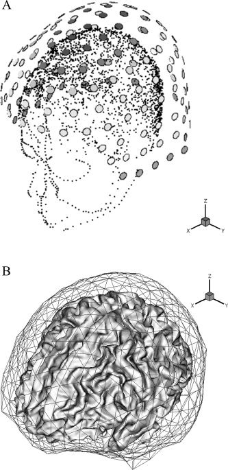
a: Sensor configuration of a 148‐channel whole head MEG system and head positions obtained from a 3‐D digitizer. b: Anatomical data used for forward/inverse calculations ‐ tessellated cortical surface and boundary element meshes (inner skull boundary). Note that the cortical surface was not included in the boundary element analysis. The cortical surface tessellation was used only for locating dipolar sources.

In this article, the boundary element method (BEM) was applied for the forward calculation of magnetic field. It has been frequently reported that just considering the inner skull boundary is sufficient for the MEG forward calculations [Meijs et al.,1988; Hämäläinen and Sarvas,1989]. The boundary surface used for the BEM was generated by commercial source analysis software (ASA v. 2.1; ANT Software) and was composed of 1,016 elements and 510 nodes. Figure 1b demonstrates the tessellated cortical surface and the boundary element meshes.

Figure 2a shows assumed fMRI activation regions obtained from a practical measurement. For the forward calculation, we placed three dipoles: two inside of the fMRI activation areas and the other outside of them. Figure 2b represents the locations of the three sources. The source intensity patterns I of three dipoles with respect to time t were defined as follows:  

Figure 2.

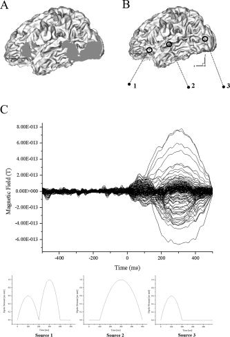
a: Assumed fMRI activation regions obtained from a practical measurement. b: Locations of three sources assumed to simulate realistic MEG signal. c: Simulated MEG signals. Real brain noise (SNR = 10) was added to each sensor. Three figures below the main signal represent source patterns.

Table  .

Source 1:
I = − 0.6 × 10‐4 (t − 100)2 + 0.6	(0 ms < t < 200 ms)
= − 10‐4 (t − 300)2 + 1	(200 ms < t < 400 ms)
= 0	(400 ms < t < 500 ms)
Source 2:
I =	0 (0 ms < t < 100 ms)
= − 0.25 × 10‐4 (t − 300)2 + 1	(100 ms < t < 500 ms).
Source 3:
I = − 0.6 × 10‐4 (t − 100)2 + 0.6	(0 ms < t < 200 ms)
= 0	(200 ms < t < 500 ms)

After the forward calculation of magnetic field assuming a 670 Hz sampling rate, we added real brain noise, which was obtained from a prestimulus period of a practical experiment. The original signal without noise was scaled in order for the signal‐to‐noise ratio to be ∼10. Figure 2c shows the finally constructed signal patterns for 148 channels with respect to simulated time.

Then we reconstructed source distributions at times of 100 ms and 300 ms using two different conditions—with and without fMRI a priori information.1 For imposing an anatomical constraint, the tessellated cortical surface was sampled to be about 10,000 dipole locations. In the simulation, we did not constrain the orientations of dipoles considering geometrical modeling error.2 Note that sources 1 and 3 were activated around 100 ms, while 1 and 2 were activated around 300 ms. Figure 3 shows the resultant source distributions at 100 ms when two assumed sources were located inside the fMRI activating areas. Throughout this article, noise normalized current dipole power (sum of squared dipole component strengths) was used for visualization purposes [Dale et al.,2000]. It can be seen from the figures that the reconstructed source distribution was further focalized by applying the fMRI constraint, which coincides well with results of a previous study [Bonmassar et al.,2001].

Figure 3.

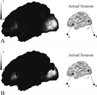
Normalized current dipole power at 100 ms (white, highest value; dark, lowest value): (a) without fMRI constraint, (b) with fMRI constraint. We can see that the distribution is more focalized by the introduction of fMRI constraint.

On the contrary, significantly different results were obtained when we applied the same procedures to data obtained at 300 ms when one source was located inside the fMRI activation areas but the other was not. Figure 4 shows the source distributions reconstructed at 300 ms. For the MEG‐alone case, the source distribution was somewhat widespread, but positions with highest source power coincide well with those of assumed dipole sources. However, when the fMRI constrained inverse procedure was applied, it can be easily seen that source 2 was nearly eliminated. Instead, nearby fMRI areas were activated to similarly mimic magnetic field distribution. This shows that the capability of reconstructing MEG sources may be degraded by the introduction of an fMRI constraint, especially when significant fMRI invisible sources exist.

Figure 4.

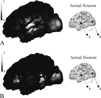
Normalized current dipole power at 300 ms (white, highest value; dark, lowest value): (a) without fMRI constraint, (b) with fMRI constraint. Source 2 outside the fMRI area was eliminated by the introduction of fMRI constraint.

In order to check the dependency of reconstructed results on the relative fMRI weighting values for fMRI inactivated areas, we varied them between 0.1, 0.3, 0.6, and 1. Figure 5 shows the changes of source distribution at 300 ms with respect to the weighting values. It can be seen from the figures that source 2 is diminished gradually according to the decrement of the relative fMRI weighting. From several simulations, including the above, we could not find any absolutely compromising value that can completely reduce distortions from the fMRI invisible sources nor prevent the fMRI invisible ones from being eliminated.

Figure 5.

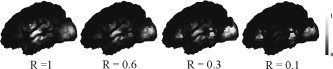
Changes of source distribution at 300 ms with respect to relative fMRI weightings. R represents relative weighting value for fMRI nonactivated regions.

Consideration of fMRI Invisible Sources

It was shown from previous simulations that some significant MEG sources that had not been detected by fMRI could be eliminated by the introduction of an fMRI constraint. In this study, we suggest that both MEG‐alone and fMRI constraint cases should be applied simultaneously for each time in consideration. Then, if the difference between two source distributions are distinguished and some sources in MEG‐alone case are eliminated by the introduction of the fMRI constraint,3 we should assess whether the missed sources are fMRI invisible ones or MEG spurious ones. In our study, for the assessment, we placed some rotating dipoles around possible activating areas. To place the dipoles, we applied the following processes:

• 1We first searched local peaks by scanning all vertices on a cortical surface. The local peak is defined as a vertex that has larger current strength than all its neighboring vertices.
• 2Some local peaks whose current strengths exceeded a predetermined threshold were selected as candidates for the dipole placement. The threshold was determined based on a noisy source‐to‐real source ratio, which will be introduced in next section.
• 3A local peak that has largest value was selected among the candidates. Some local peaks that are close to the selected one were excluded from the candidate set. The critical distance to discriminate sources was determined using a statistical method. Fujimaki et al. [2002] performed numerous simulations for the same sensor configuration as in this study, and selected 40 mm as the separation threshold, because the probability of finding dipole pairs with high crosstalk (over 50%) decreases to as low as 5.6% at that distance. In this study, the same separation threshold was applied to place the rotating dipoles.
• 4Then process (3) was repeated until no candidates were left. These processes were applied to both MEG‐alone case and fMRI constraint case. If the distances among dipoles are less than the separation threshold, we selected dipoles from MEG‐alone case.

Then, temporal changes of the dipoles' moment vectors were estimated using truncated singular value decomposition (tSVD), which allows the solutions to satisfy a condition of least squares for errors in magnetic fields. If the magnitude of an estimated dipole moment has a smaller value than a noise level, we judged that the distributed sources around the dipole have high probability to be spurious sources. Such an assessment using small numbers of dipoles is thought reasonable because such estimations have a much smaller probability to generate spurious solutions compared to the distributed source models that use large numbers of dipoles simultaneously.

To check this property, we placed four dipoles at probable activation regions, as shown in Figure 6a. Figure 6b shows the temporal changes of the testing dipoles around 300 ms, where the missed source 2 shows significant dipole moment intensity. Therefore, it has large probability to be an fMRI invisible source, not just a spurious source. In this way, we can assess whether the sources missed during fMRI constrained inverse processes are meaningful ones or ignorable ones.

Figure 6.

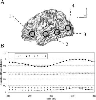
a: Placement of four rotating dipoles to check whether missed source 2 is an fMRI invisible source or just a spurious one. b: Temporal changes of source intensities for the four rotating dipoles.

Application to a Japanese Language Lexical Judgment Test

A problem considered in this study was a Japanese language lexical judgment test [Fujimaki et al.,1999]. Several strings of three characters were visually presented to a subject (a right‐handed Japanese). The set of strings was composed of Japanese katakana strings (meaningful nouns) and meaningless pseudo‐character strings. The subject answered whether the strings were meaningful or not by pressing one of two buttons with his left index and middle fingers. The visual stimuli were presented below a square (a fixation mark) every 2 s with a duration of 1 s. Luminance was 15 cd/m² for the stimulus and 0.5 cd/m² for the background, and the visual angle was 1.3° for one character and 0.3° for the fixation mark. A 1.5 T fMRI system (Magnetom Vision, Siemens, Erlangen, Germany) using an echo planar imaging method with parameters TR 12.65 s, TE 66 ms, pixels 2.2 × 2.2 mm, slice thickness 7 mm, and slice gaps 2.8 mm. The fMRI data were analyzed using imaging processing software (SPM99); they were preprocessed by motion correction and co‐registered to the subject's T1 structural image. For the control condition of fMRI, the subject was visually presented with single pseudo‐characters or just a fixation mark, and answered whether the characters were presented or not, which was a visual form process requiring a smaller load than the test condition.

For the MEG experiment, we applied the same conditions as the fMRI case. A 148‐channel whole head system was used to record the magnetic field, which was already presented in the previous forward simulations. The data were averaged over 200 epochs (pre‐trigger period: 500 ms, post‐trigger period: 1,200 ms) and were filtered with a bandpass of 0.3 to 40 Hz. Figure 7a shows the measured MEG waveform.

Figure 7.

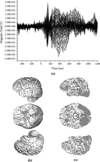
a: MEG waveform measured with 148‐channel magnetometers from one subject. Over 200 epochs of data were averaged and filtered with a bandpass of 0.3 to 40 Hz. b: Result of fMRI SPM analysis. c: fMRI activation regions coregistered with a tessellated cortical surface.

For the MEG signal analysis, we applied the boundary element method (BEM) for forward calculation and tessellated cortical surface for inverse reconstruction, as in the previous simulations (Fig. 1a,b). To apply the fMRI constrained MEG inverse process, we first projected fMRI activation regions into the tessellated cortical surface. Figure 7b shows the result of fMRI statistical parametric mapping (SPM). Figure 7c depicts the fMRI activation regions coregistered with the tessellated cortical surface.

Considering temporal changes of magnetic field distribution on a sensor plane, we reconstructed MEG source distributions at 80 and 140 ms. This article will not deal with or discuss the meanings of reconstructed results and will show just the difference between MEG‐alone and fMRI constraint cases because this topic has not been fully discussed yet. However, it is expected that visual form neural activations will occur around 80 ms and left‐hemisphere dominance will be observed around 140 ms, as in other visual and phonological experiments studied before [Fujimaki et al.,2002]. Figure 8a shows the magnetic field map on a sensor plane and reconstructed source distributions4 with and without fMRI constraint at 80 ms. We can see from the results that earliest visual activations were observed as expected, and the extended sources were focalized more by the introduction of the fMRI constraint. Figure 8b also shows the magnetic field map and source distributions at 140 ms. We could observe that MEG extended sources inside fMRI activation regions were focalized by the introduction of the fMRI constraint, but some MEG sources outside the regions were eliminated as in the previous simulation studies. Therefore, we placed some regional sources around possible activation regions. Eight rotating dipoles were placed as shown in Figure 9a and their temporal changes were investigated using tSVD between 120 and 160 ms. Figure 9b shows the normalized dipole intensities with respect to time.

Figure 8.

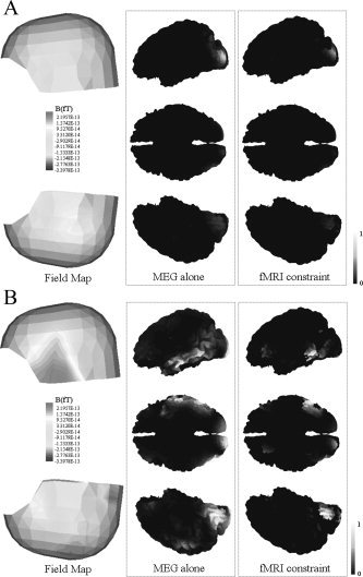
Magnetic field map and MEG source distributions with and without fMRI constraint (lower figures): (a) at 80 ms; (b) 140 ms. Viewpoints are the same as those in Figure 7c.

Figure 9.

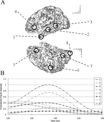
a: Locations of regional sources to check temporal changes of possible activations. b: Temporal changes of regional dipoles with respect to time.

Since the magnitudes of measured signals did not necessarily coincide with estimated source intensities,5 we estimated a noisy source‐to‐real source ratio in order to assess significance of a regional source. First, we selected several points of time in a noise window, reconstructed source distributions using anatomical constraints, and checked their maximum magnitudes. Then, we applied the same processes to a signal window. By comparing magnitudes of noisy and real sources, we found that the noisy source intensity did not exceed 15% of maximum (real) source intensity, which appears around 140 ms. The estimated ratio was used to check whether the eliminated sources were real MEG generators or just spurious sources.

From Figure 9b, we could see the following:

• Regional sources 1, 2, 5, and 6 were located around missed activations. Dipole intensities of 1 and 2 were large, while those of 5 and 6 were smaller than the noisy source level defined above.

• Other dipoles (3, 4, 7, and 8), which were located inside fMRI activation regions, also showed relatively significant levels at 140 ms, compared to the noisy source level.

• Hence, we could conclude that the missed sources 1 and 2 have larger probability to be fMRI invisible sources, but 5 and 6 may be spurious sources, which were generated during MEG inverse processes.

Inspiringly, the finally estimated dipole locations coincide well with the previous study on a phonological judgment test [Fujimaki et al.,2002].

CONCLUSIONS

In this article fMRI constrained MEG source reconstruction was implemented and applied to simulation and experiment studies. From the results, we found that the conventional technique to impose fMRI constraint using “a diagonal weighting” could miss some significant fMRI invisible MEG sources and some distortions stemming from the missed sources were unavoidable even when the value of the diagonal weighting was adjusted.

If no fMRI invisible sources exist, i.e., the fMRI activation regions can cover every MEG generator, the MEG source distribution could be focalized by fMRI constraint. Moreover, the use of fMRI prior information could eliminate spurious sources generated due to an ill‐posed MEG inverse problem and the MEG analysis could provide temporal information for the fMRI results. However, these merits may become useless when there are significant MEG generators that are not included in fMRI activations. In this article we suggested that one should simulate both MEG‐alone case as well as fMRI constraint case and should compare the two results. If the difference is distinguished and some sources are eliminated by the introduction of fMRI constraint, small numbers of regional sources were placed around all possible candidate positions and their temporal changes were investigated. If the magnitude of a dipole vector exceeds a noisy level, it has large probability to be an fMRI invisible source; if not, it may be a spurious source that usually stems from the ill‐posed characteristic of typical MEG inverse problems.

We can summarize possible cases as follows:

• 1Peak positions from an fMRI constraint case and those from a MEG‐alone case are identical: In this case, one can trust results from fMRI constrained MEG analysis.
• 2Peak positions from an fMRI constraint case and those from a MEG‐alone case are not identical and some MEG sources are eliminated by the fMRI constraint. After the regional source test, all the missing sources are proved to be MEG spurious sources: One can trust results from fMRI constrained MEG analysis as well.
• 3Peak positions from an fMRI constraint case and those from a MEG‐alone case are not identical and some MEG sources are eliminated by the fMRI constraint. After the regional source test, some of the missing dipoles have significant dipole moments: One cannot fully trust results from fMRI constrained MEG analysis. In this case, one can use the results of a regional dipole test to estimate real source locations.

We expect that this method can be a very promising method to find neuronal activities that could not be detected by conventional fMRI constrained MEG or fMRI‐alone analyses. Further studies should be continued to develop new techniques to consider fMRI invisible sources as well as to take full advantage of fMRI a priori information.

REFERENCES

- Ahlfors SP, Simpson GV, Dale AM, Belliveau JW, Liu AK, Korvenoja A, Virtanen J, Huotilainen M, Tootell RBH, Aronen HJ, Ilmoniemi RJ (1999): Spatiotemporal activity of a cortical network for processing visual motion revealed by MEG and fMRI. J Neurophysiol 82: 2545–2555. [DOI] [PubMed] [Google Scholar]
- Baillet S, Riera JJ, Marin G, Mangin JF, Aubert J, Garnero L (2001): Evaluation of inverse methods and head models for EEG source localization using a human skull phantom. Phys Med Biol 46: 77–96. [DOI] [PubMed] [Google Scholar]
- Bonmassar G, Schwartz DP, Liu AK, Kwong KK, Dale AM, Belliveau JW (2001): Spatiotemporal brain imaging of visual‐evoked activity using interleaved EEG and fMRI recordings. NeuroImage 13: 1035–1043. [DOI] [PubMed] [Google Scholar]
- Dale AM, Sereno M (1993): Improved localization of cortical activity by combining EEG and MEG with MRI surface reconstruction: a linear approach. J Cogn Neurosci 5: 162–176. [DOI] [PubMed] [Google Scholar]
- Dale AM, Liu AK, Fischl BR, Buckner RL, Belliveau JW, Lewine JD, Halgren E (2000): Dynamic statistical parametric mapping: combining fMRI and MEG for high‐resolution imaging of cortical activity. Neuron 26: 55–67. [DOI] [PubMed] [Google Scholar]
- Fuchs M, Wagner M, Kohler T, Wischmann H‐A (1999): Linear and nonlinear current density reconstructions. J Clin Neurophysiol 16: 267–295. [DOI] [PubMed] [Google Scholar]
- Fujimaki N, Miyauchi S, Putz B, Sasaki Y, Takino R, Sakai K, Tamada T (1999): Functional magnetic resonance imaging of neural activity related to orthographic, phonological and lexico‐semantic judgments of visually presented characters and words. Hum Brain Mapp 8: 44–59. [DOI] [PMC free article] [PubMed] [Google Scholar]
- Fujimaki N, Hayakawa T, Nielsen M, Knösche TR, Miyauchi S (2002): An fMRI‐constrained MEG source analysis with procedures for dividing and grouping activation. NeuroImage 17: 324–343. [DOI] [PubMed] [Google Scholar]
- George J, Mosher JC, Schmidt D, Aine C, Wood C, Lewine J, Sanders J, Belliveau J (1995): Functional neuroimaging by combined MRI, MEG and fMRI. Hum Brain Mapp S1: 89. [Google Scholar]
- Hämäläinen MS, Ilmoniemi RJ (1984): Interpreting measured magnetic fields of the brain: estimates of current distributions. Technical Report TKK‐F‐A559, Helsinki University of Technology.
- Hämäläinen MS, Sarvas J (1989): Realistic conductivity geometry model of the human head for interpretation of neuromagnetic data. IEEE Trans Biomed Eng 36: 165–171. [DOI] [PubMed] [Google Scholar]
- Horwitz B, Poeppel D (2002): How can EEG/MEG and fMRI/PET data be combined? Hum Brain Mapp 17: 1–3. [DOI] [PMC free article] [PubMed] [Google Scholar]
- Im C‐H, An K‐O, Jung H‐K, Kwon H, Lee Y‐H (2003): Assessment criteria for MEG/EEG cortical patch tests. Phys Med Biol 48: 2561–2573. [DOI] [PubMed] [Google Scholar]
- Kincses WE, Braun C, Kaiser S, Elbert T (1999): Modeling extended sources of event‐related potentials using anatomical and physiological constraints. Hum Brain Mapp 8: 182–193. [DOI] [PMC free article] [PubMed] [Google Scholar]
- Korvenoja A, Huttunen J, Salli E, Pohjonen H, Martinkauppi S, Palva JM, Lauronen L, Virtanen J, Ilmoniemi RJ, Aronen HJ (1999): Activation of multiple cortical areas in response to somatosensory stimulation: combined magnetoencephalographic and functional magnetic resonance imaging. Hum Brain Mapp 8: 13–27. [DOI] [PMC free article] [PubMed] [Google Scholar]
- Liu AK, Belliveau JW, Dale AM (1998): Spatiotemporal imaging of human brain activity using functional MRI constrained magnetoencephalography data: Monte Carlo simulations. Proc Natl Acad Sci U S A 95: 8945–8950. [DOI] [PMC free article] [PubMed] [Google Scholar]
- Liu AK, Dale AM, Belliveau JW (2002): Monte Carlo simulation studies of EEG and MEG localization accuracy. Hum Brain Mapp 16: 47–62. [DOI] [PMC free article] [PubMed] [Google Scholar]
- Matsuura K, Okabe Y (1995): Selective minimum‐norm solution of the biomagnetic inverse problem. IEEE Trans Biomed Eng 42: 608–615. [DOI] [PubMed] [Google Scholar]
- Meijs JW, Peters MJ, Boom HB, Lopes da Silva FH (1988): Relative influence of model assumptions and measurement procedures in the analysis of the MEG. Med Biol Eng Comput 26: 136–142. [DOI] [PubMed] [Google Scholar]
- Scherg M (1992): Functional imaging and localization of electromagnetic brain activity. Brain Topogr 5: 103–111. [DOI] [PubMed] [Google Scholar]
- Shattuck DW, Leahy RM (2002): BrainSuite: an automated cortical surface identification tool. Med Image Anal 6: 129–142. [DOI] [PubMed] [Google Scholar]