Automated analysis of meta‐analysis networks

Abstract

The high information content in large data sets from voxel‐based meta‐analyses is complex, making it hard to readily resolve details. Using the meta‐analysis network as a standardized data structure, network analysis algorithms can examine complex interrelationships and resolve hidden details. Two new network analysis algorithms have been adapted for use with meta‐analysis networks. The first, called replicator dynamics network analysis (RDNA), analyzes co‐occurrence of activations, whereas the second, called fractional similarity network analysis (FSNA), uses binary pattern matching to form similarity subnets. These two network analysis methods were evaluated using data from activation likelihood estimation (ALE)‐based meta‐analysis of the Stroop paradigm. Two versions of these data were evaluated, one using a more strict ALE threshold (P < 0.01) with a 13‐node meta‐analysis network, and the other a more lax threshold (P < 0.05) with a 22‐node network. Java‐based applications were developed for both RDNA and FSNA. The RDNA algorithm was modified to provide multiple subnets or maximal cliques for meta‐analysis networks. Three different similarity measures were evaluated with FSNA to form subsets of nodes and experiments. RDNA provides a means to gauge importance of metanalysis subnets and complements FSNA, which provides a more comprehensive assessment of node similarity subsets, experiment similarity subsets, and overall node‐to‐factors similarity. The need to use both presence and absence of activations was an important finding in similarity analyses. FSNA revealed details from the pooled Stroop meta‐analysis that would otherwise require separate highly filtered meta‐analyses. These new analysis tools demonstrate how network analysis strategies can simplify greatly and enhance voxel‐based meta‐analyses. Hum Brain Mapp 25:174–184, 2005. © 2005 Wiley‐Liss, Inc.

INTRODUCTION

Functional imaging studies map brain activity during task performance; however, well‐controlled tasks almost always activate multiple brain regions, commonly designated “distributed neural networks.” By this terminology, individual brain regions can be considered nodes within a network. Location, extent, and activation level vary across individuals and studies; therefore, standardization is needed to understand better the nature of such networks. This standardization is provided by a meta‐analysis network, defined as a set of nodes from a voxel‐based meta‐analysis. A formal means to create a meta‐analysis network using the activation likelihood estimation (ALE) method was introduced by Turkeltaub et al. [2002]. ALE determines 3‐D volumes of interest (VOIs) from coordinate locations in studies of the voxel‐based meta‐analysis. Each VOI represents extent and location of a network node in standardized brain space, and the full set of VOIs forms the meta‐analysis network. Meta‐analysis networks defined in this format provide a stable framework for the application of existing and development of novel network analysis algorithms.

Formal brain network analysis often has focused on bottom‐up strategies [Bower et al.,1998] where networks evolve from neuron models. Top‐down approaches, where network nodes and interconnectivity are deduced from spatial–functional relationships, are more appropriate for analysis of meta‐analysis networks. Unfortunately, the large complex data sets associated with meta‐analyses present an overwhelming task for researchers, leaving many relationships within the data undiscovered. Top‐down network analysis strategies provide tools to filter quickly through such data sets and new ways to view relationships within these data. An exciting proposition is that these network analysis tools will reveal new relationships in meta‐analysis networks. Several new meta‐analysis network analysis methods and associated processing tools are reviewed in the present study.

A clique, which is a mutually connected subset of nodes, is an important structural feature used in characterizing networks [Pelillo et al.,1999]. In fact, the maximal clique, a clique not contained within another clique, has been used as the basis for comparing 3D molecular structures [Gardiner et al.,1998] and in particular for proteins [Samudrala and Moult,1998]. Replicator dynamics [Bomze and Pelillo,2000] can be used to determine a maximal weighted clique from arbitrary undirected and weighted network graphs. In this issue, Neumann et al. [2005] present a threshold version of replicator dynamics network analysis (RDNA) that determines a “dominant network” for a Stroop meta‐analysis network. There are many algorithms yet to be explored for analyzing meta‐analysis networks, and an especially attractive approach is based on classic pattern‐matching techniques [Anderberg,1973; Johnson and Wichern,1988]. Subsets of similar nodes and experiments are the outcome of the new pattern‐matching method called fractional similarity network analysis (FSNA). Unlike RDNA, which only finds a single subset of nodes, the FSNA pattern matching method leads to complete subsets of the data and mimics pattern‐matching activities that researchers use when carrying out meta‐analyses. The structured approach provided by automated analysis of large complex data sets increases the likelihood of discovery of obscure patterns.

When multiple studies are pooled in a voxel‐based ALE meta‐analysis, not all regions (network nodes) are activated in each contributing study (e.g., see Table II in Turkeltaub et al. [2002] and Table VI in Laird et al. [2005a]). Although it is possible that the pattern of presences/absences is random, it is far more likely that occurrence patterns are meaningful, reflecting interpretable variations among the studies. Experimental variations reasonably expected to influence the reproducibility of activations and the specific patterns elicited include: differences in the experimental paradigm used (task and control states), the wording of the instructions to the subject, the amount of training given to subjects, the subject population (e.g., age, gender, handedness, educational level, task skill level, or other factors), the brain imaging modality used, the imaging field of view (i.e., if less than whole brain), the sample size of each study, and the statistical threshold applied in reporting activations. Consequently, tools for exploring occurrence patterns should be valuable for the neuroscientific and technical interpretation of voxel‐based meta‐analyses.

Table II.

Node summary for pooled ALE‐P01Stroop meta‐analysis

Node	x	y	z	Experiments/node	Volume (mm3)	Anatomical label	Brodmann area
1	1	16	38	11	4,288	R anterior cingulate	32
2	−44	5	33	8	1,680	L inferior frontal gyrus	9
3	−40	−50	44	3	992	L inferior parietal lobule	40
4	−42	23	10	5	744	L inferior frontal gyrus	13
5	−48	9	11	4	696	L inferior frontal gyrus	44
6	−21	−72	36	4	552	L precuneus	7
7	46	9	28	3	448	R inferior frontal gyrus	9
8	−3	38	25	2	360	L anterior cingulate	32
9	36	12	7	3	312	R insula	13
10	20	48	23	2	272	R superior frontal gyrus	10
11	−42	30	31	3	200	L mid frontal gyrus	9
12	−45	−42	36	2	192	L supramarginal gyrus	40
13	−26	22	5	1	184	L insula (claustrum)	—

Table VI.

Profile of all nodes for pooled ALE‐P01 Stroop meta‐analysis

Node	Control				Response		P threshold			Group size (n)
	Congruent	Neutral	Nonlexical	Combo	Verbal	Manual	<0.05	<0.005	<0.001	>20	10 < n < 20	<10
1	0.421	0.474	0.421	0.526	0.474	0.526	0.579	0.368	0.421	0.421	0.421	0.579
2	0.474	0.632	0.474	0.579	0.211	0.789	0.421	0.526	0.474	0.579	0.684	0.421
3	0.526	0.684	0.737	0.737	0.368	0.632	0.158	0.579	0.737	0.842	0.421	0.158
4	0.526	0.474	0.737	0.737	0.474	0.526	0.263	0.579	0.632	0.737	0.421	0.263
5	0.474	0.526	0.789	0.789	0.526	0.474	0.211	0.526	0.684	0.789	0.263	0.211
6	0.474	0.737	0.684	0.684	0.211	0.789	0.211	0.421	0.684	0.789	0.474	0.211
7	0.526	0.684	0.737	0.737	0.368	0.632	0.158	0.579	0.737	0.842	0.421	0.158
8	0.474	0.632	0.895	0.789	0.316	0.684	0.105	0.526	0.789	0.789	0.263	0.105
9	0.421	0.684	0.842	0.737	0.474	0.526	0.158	0.684	0.842	0.737	0.316	0.158
10	0.579	0.632	0.789	0.789	0.421	0.579	0.105	0.632	0.789	0.895	0.368	0.105
11	0.526	0.579	0.737	0.843	0.368	0.632	0.158	0.684	0.737	0.842	0.421	0.158
12	0.368	0.737	0.895	0.789	0.316	0.684	0.105	0.526	0.789	0.895	0.368	0.105
13	0.421	0.684	0.947	0.842	0.368	0.632	0.053	0.579	0.842	0.842	0.211	0.053
Max	0.579	0.737	0.947	0.842	0.526	0.789	0.579	0.684	0.842	0.895	0.684	0.579
Mean	0.478	0.628	0.745	0.737	0.377	0.623	0.207	0.555	0.704	0.769	0.389	0.207
Median	0.474	0.632	0.737	0.737	0.368	0.632	0.158	0.579	0.737	0.789	0.421	0.158
Min	0.368	0.474	0.421	0.526	0.211	0.474	0.053	0.368	0.421	0.421	0.211	0.053

Boldface type indicates highest similarity in each of the control and response subcategories. Mean values are also in boldface type.

Theory

An experiment table (Fig. 1) is the starting point for both RDNA and FSNA. It summarizes presence (1) or absence (0) of nodes in each experiment for an ALE meta‐analysis. Summing the values of 1 across rows in this table determines node incidence. In the table of Figure 1, node 3 has the highest incidence. Likewise, summing the values of 1 in columns shows that Experiments 1 and 5 had three nodes whereas other experiments had two nodes. Binary patterns from rows can be used to assess similarity between nodes; likewise, column binary patterns can be used to assess similarity between experiments. Similarity measures used in clustering algorithms for binary patterns are defined most often using binary matching as summarized in Table I [Johnson and Wichern,1988]. The similarity measure that tabulates only 1–1 matches between binary patterns (a from Table I) is the basis for calculating the co‐occurrence matrix used by RDNA, as only co‐active nodes are considered relevant. Similarly, values for b, c, and d are sums for 0–1, 1–0, and 0–0 conditions between two binary patterns.

Figure 1.

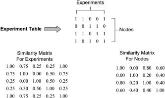
Meta‐analysis network experiment table and S1 type similarity matrices for experiments and nodes.

Table I.

Binary matching

	1	0
1	a	b	a + b
0	c	d	c + d
	a + c	b + d	a + b + c + d

FSNA pattern analysis

Three similarity coefficients (S1, S2, and S3) were selected to assess pattern similarity in meta‐analysis networks by FSNA. The first coefficient is the fraction of 1–1 and 0–0 matches between two patterns and is calculated as S1 = (a + d)/(a + b + c + d) from Table I. The denominator of this coefficient is the sum of experiments or nodes, depending on the pattern type being evaluated. This simple similarity coefficient is the most general and provides a baseline measure of similarity. The second similarity coefficient S2 is the fraction of 1–1 matches, treating 0–0 pairs as nonrelevant. It is calculated as S2 = a/(a + b + c), and is also called the Jaccard similarity measure [Anderberg,1973]. The third similarity coefficient S3 tabulates only 1–1 matches, as is done for the co‐occurrence matrix. Its similarity fraction is calculated as S3 = a/(a + b + c + d). S3 is also known as the Russel and Rao similarity measure or binary dot product [Anderberg,1973]. Figure 1 illustrates matrices of S1 similarity coefficients that are naturally symmetric.

Numerous other similarity measures for binary patterns are possible, including Euclidean distance (D) and the Pearson's correlation coefficient (R). A common measure used for clustering of binary patterns is D² = b + c [Anderberg,1973], but because it is a measure of dissimilarity we opted for S1. Pearson's correlation coefficient is more useful with continuous data although simple formulae are available for this calculation with binary patterns [Johnson and Wichern,1988]. R is less versatile when compared to S1–S3 similarity measures, and it is not used often as the basis for binary valued clustering as needed for FSNA.

FSNA subset clustering algorithm

A hierarchical clustering algorithm forms subsets, each with members more similar to each other than to members of other subsets. The first step in the clustering algorithm is to form a subset of patterns with the highest similarity. Nonclustered patterns are evaluated similarly until all patterns are members of a subset. Matching is only allowed for fractional similarity greater than one‐half in this example. In the experiment S1 similarity matrix of Figure 1, Experiments 1 and 5 have the highest similarity coefficient, so subset (1,5) is formed. The next highest similarity is between Experiment 2 and Experiments 1 and 5. Because Experiments 1 and 5 are in the same subset, Experiment 2 is appended as a new member forming subset (1,2,5). The next highest fractional similarity (0.5) is insufficient for clustering so Experiments 3 and 4 remain as isolated subsets, which completes the clustering. In this case, the clustering algorithm reduced the initial five experiments to three similarity subsets: (1,2,5), 3, and 4. Clustering using the node S1 similarity matrix in Figure 1 leads to two subsets of nodes (1,3,4) and 2. Using S2 similarity, the same clustering is seen for experiments, but nodes cluster as subsets (1,3), 2, and 4. Finally, S3‐type similarity produces clustering similar to S2 for nodes but different for experiments as (1,5), 2, 3, and 4. This hierarchical clustering algorithm is bias free, with the number of subsets and membership determined by ranking of similarity coefficients and the clustering threshold. Similarity coefficients in this example were assumed to be distributed uniformly with a mean of 0.5. The clustering threshold of >0.5 ensured that clustering was done with greater than chance similarity. Mean values for S1–S3 similarity coefficients of the larger patterns seen with meta‐analysis data were naturally distributed more widely, requiring corresponding changes in cluster thresholds, described below.

Maximal clique

A clique is defined formally from a network's graph as a subset in which all nodes are mutually adjacent [Pelillo et al.,1999], i.e., every node is connected directly to every other node in the subset (Fig. 2). A maximal clique is one that is not contained in any other cliques. The maximum clique is the maximal clique with the largest number of nodes. As a practical example, a maximal clique within an ad hoc cell‐phone network is the set of cells that are actively communicating when providing phone service. This is important, as other cells must not interfere when cells of the maximal clique are active, and this requirement may hold for distributed neural networks. Maximal cliques have also been used as the basis for comparing 3‐D molecular structures [Gardiner et al.,1998] and in particular for proteins [Samudrala and Moult,1998]. Protein structure cliques are determined using graph‐theory maximal clique algorithms and associated network graphs. With only associations between nodes, as is the case with meta‐analysis networks, alternative methods based on replicator dynamics approach have been utilized to determine maximal weighted cliques [Bomze and Pelillo,2000; Pelillo et al.,1999]. Replicator dynamics has also been used with functional magnetic resonance imaging (fMRI) data to find coherent subnets where each node is claimed to be “as close to as many other nodes as possible” [Lohmann and Bohn,2002], with closeness (node similarity) defined using Spearman's rank correlation. Neumann et al. [2005] suggest that the maximal weighted clique for a meta‐analysis network is the “dominant network” and will “likely play a critical role in an investigated cognitive task.” Because of the nonzero threshold of 1/n (n = number of elements in a pattern) used in determining clique membership with replicator dynamics [Lohmann and Bohn,2002; Neumann et al.,2005] the result may be a subset of the maximal clique, although in many studies maximal cliques have been reported consistently [Bomze and Pelillo,2000; Pelillo et al.,1999].

Figure 2.

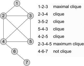
Examples of clique, maximal clique, and maximum clique for a simple network.

MATERIALS AND METHODS

Data

Data for testing RDNA and FSNA were taken from the pooled Stroop ALE meta‐analysis carried out by Laird et al. [2005a,b], which used 205 foci from 19 experiments. Two subsets of this data were formed, one using a false discovery rate (FDR)‐corrected ALE cluster threshold of P < 0.01 (ALE‐P01), which provided a meta‐analysis network of 13 nodes or VOIs. The second dataset was created using ALE with a less restrictive FDR‐corrected threshold of P < 0.05 (ALE‐P05) and resulted in a meta‐analysis network of 22 nodes. Table II and Table III summarize node and experiment data for the ALE‐P01 Stroop meta‐analysis. Nodes were numbered according to volume. Talairach coordinates in Table II were used in conjunction with the Talairach Daemon [Lancaster et al.,2000] to determine anatomical labels. The only change was that Node 1 was designated anterior cingulate though its Talairach Daemon label was cingulate cortex.

Table III.

Experiment summary for pooled ALE‐P01 Stroop meta‐ analysis

Experiment	Nodes/ experiment	Author*	Control type	Response type	Modality	Statistics		Subjects (n)
						Type	P
1	1	Taylor	Neutral	Verbal	PET	t, z	<0.001	10 < n < 20
2	2	Carter, 1995	Congruent	Verbal	PET	t, z	<0.005	10 < n < 20
3	1	Derbyshire	Congruent	Verbal	PET	t, z	<0.001	<10
4	0	Bench	Neutral	Verbal	PET	t, z	<0.05	<10
5	5	Leung	Congruent	Verbal	ER fMRI	t, z	<0.005	10 < n < 20
6	3	Brown	Combination	Verbal	Block fMRI	t, z	<0.05	<10
7	8	Peterson, 1999	Congruent	Verbal	Block fMRI	t, z	<0.05	>20
8	1	Carter, 2000	Congruent	Verbal	ER fMRI	Other	<0.01	10 < n < 20
9	0	MacDonald	Congruent	Verbal	Block fMRI	Other	<0.005	10 < n < 20
10	4	Banich	Neutral	Manual	Block fMRI	Other	<0.05	10 < n < 20
11	5	Steel	Nonlexical	Verbal	Block fMRI	Other	<0.01	<10
12	4	Milham, 2001	Neutral	Manual	ER fMRI	t, z	<0.05	10 < n < 20
13	3	Milham,2002	Combination	Manual	Block fMRI	Other	<0.0025	10 < n < 20
14	1	Mead	Congruent	Manual	Block fMRI	t, z	<0.05	10 < n < 20
15	2	George	Nonlexical	Verbal	PET	t, z	<0.01	>20
16	1	Pardo	Congruent	Verbal	PET	t, z	<0.01	<10
17	3	Fan	Congruent	Manual	ER fMRI	t, z	<0.05	10 < n < 20
18	4	Peterson, 2002	Congruent	Verbal	ER fMRI	t, z	<0.005	10 < n < 20
19	3	Ruff	Neutral	Manual	Block fMRI	t, z	<0.05	10 < n < 20

^*References are provided in Laird et al.,2005a.

RDNA

Neumann et al. [2005] provide an excellent discussion of the methods involved in using replicator dynamics with an ALE meta‐analysis, and we subsequently developed a Java application based on their methodology. ALE VOIs were formed using the method described by Laird et al. [2005b]. These VOIs are used to inspect coordinates from each experiment to determine the nodes that are active (1) and inactive (0). Results are tabulated and stored in an experiment table following the format in Table I. The experiment table is analyzed to formulate a matrix of co‐occurrence values for each pair of nodes. From the co‐occurrence matrix, RDNA determines a maximal clique for the meta‐analysis network. Verification of the maximal clique algorithm in the RDNA application was done using the example experiment table and co‐occurrence matrix from Neumann et al. [2005]. Although Neumann et al. [2005] reports only a single dominant network, Lohmann and Bohn [2002] described a method for determining additional networks using replicator dynamics that was applicable in fMRI data, not meta‐analysis networks. RDNA software was modified so that multiple maximal cliques could be determined from a meta‐analysis network. The algorithm assumes that the co‐occurrence matrix is a summation of co‐occurrences from subnetworks, each of which is a maximal clique. After the determination of the first maximal clique, its co‐occurrences are subtracted from the co‐occurrence matrix and the processing is repeated to find the next maximal clique. This recursive approach continues until no further maximal cliques can be determined. An important feature of RDNA is that the first maximal clique theoretically is the most important, with each subsequent clique having diminished importance.

FSNA Threshold

The mean S1 similarity coefficient (∼0.6) was much larger than were the S2 and S3 coefficients. The operational clustering threshold used for S1 similarity was 0.5 and clustering was always complete above a coefficient of 0.6. The S2 coefficient was slightly larger than the S3 coefficient was, but their average across all studies was very low (∼0.10). The small similarity fractions for these measures resulted from the low incidence of active nodes reported in many of the Stroop experiments (Table II and III). The operational clustering threshold for S2 and S3 was set at zero. All clustering using S2 and S3 similarity was complete well above this threshold and slightly above the mean similarity coefficient (0.10). Our choice of threshold was to let the data naturally cluster above the threshold. In fact, we could have used a threshold of zero without any change in outcome, so we feel that this was a reasonable threshold strategy.

FSNA Clustering

For the large node and experiment patterns, the clustering strategy was augmented using a voting paradigm where patterns with n highest similarity coefficients had n votes. Indices of the highest similarity coefficients indicated which pattern the votes were for. The pattern having the most votes was clustered first. A slightly different approach was preferred for node clustering, where node size determined voting order. During clustering, votes were tallied and the pattern (node or experiment) was moved to the subset receiving the most votes. If none of the votes were for members of subsets, then a new subset was formed to include the voting pattern and all those receiving votes. In cases of ties, additional votes were tallied using the next highest similarity coefficients. This clustering approach successfully formed clusters for all data evaluated.

FSNA Application

A Java application similar to that for RDNA was developed for FSNA. Similarity measures for all pairs of patterns in the experiment table were organized into two matrices using this software, one tabulating similarity between experiments and the other similarity between nodes (Fig. 1). These similarity matrices are square and symmetric with dimension equal to the number of experiments or nodes. For the experiment similarity matrix in Figure 1, the similarity coefficient at row 2 and column 5 is 0.75. This is the S1 similarity coefficient comparing experiment binary patterns in columns 2 and 5 of the experiment table. Likewise the value in row 2 and column 4 in the node similarity matrix is 0.40. This is the S1 similarity coefficient comparing node binary patterns in rows 2 and 4 of the experiment table.

Experiments

Large experiment tables similar the one in Figure 1, derived from the 19 experiments of the pooled Stroop meta‐analysis, were formulated for ALE‐P01 and ALE‐P05 data sets. Each experiment table was processed using RDNA to determine maximal cliques. Each experiment table was also processed using FSNA to determine node and experiment subsets. Similarity coefficient matrices similar to those in Figure 1 were generated using S1, S2, and S3 similarity coefficients. The FSNA clustering algorithm was applied to the similarity coefficient matrices to create similarity subsets.

RESULTS

Node Clustering

The stricter ALE‐P01 threshold produced fewer nodes than did the ALE‐P05 threshold (13 vs. 22) and this led to fewer subsets (Table IV). RDNA cliques in Table IV are ordered according to their number of occurrences (in parenthesis) and FSNA similarity subsets by average similarity. Not all cliques are tabulated as many were found (19 for ALE‐P01 data and 38 for ALE‐P05 data). S3 similarity failed to form multiple subsets for either ALE‐P01 or ALE‐P05 data.

Table IV.

Node subsets for Stroop meta‐analysis networks

RDNA Maximal cliques	FSNA
	S1 similarity	S2 similarity
ALE‐P01 (13 nodes)
1,2 (6)	3,6,10	3,6,10
1,2,6,7,11 (1)	4,5,8,9,12,13	7,11
1,4,5 (2)	1,2,7,11	8,13
2,3,6 (2)		1,2
		4,5,9,12
ALE‐P05 (22 nodes)
1,2,4,7,9 (3)	8,13a, b	13a, b
1,2,3,6 (3)	1,2,7,11,19,21	11,19,21
3,4,9,10 (2)	20,22	20,22
1,9,11,19,21 (1)	17,18	4,8,9
4,6,8,16 (1)	15,16	3,10
2,11,20,22 (1)	4,9	17,18
	3,10	1,2,7
	6,14	6,14,15,16

^aNo corresponding ALE‐P01 node; right posterior cingulate, Brodmann area 23.

^bNo corresponding ALE‐P01 node; right precuneus, Brodmann area 7.

ALE‐P01 data

RDNA.

For the ALE‐P01 data, RDNA reported the first maximal clique as nodes (1,2), much smaller than the five‐node dominant network reported by Neumann et al. [2005]. Removal of occurrences from the high incidence (1,2) clique by RDNA led to a five‐node maximal clique consistent with the five‐node network reported by Neumann et al. [2005]. This second maximal clique (1,2,6,7,11) contained the (1,2) clique and therefore was considered more important in the ALE‐P01 meta‐analysis network. The additional nodes (6,7,11) in the second maximal clique were not just those of next highest incidence. Importantly, the second maximal clique (1,2,6,7,11) was more like the S1 (1,2,7,11) and S2 (1,2)(7,11) similarity subsets determined by FSNA. The (1,2) maximal clique was reported as the (1,2) S2 similarity subset and the (1,4,5) and (2,3,6) maximal cliques were found in separate S2 similarity subsets, indicating that smaller maximal cliques are more like S2 similarity subsets than like S1 subsets for this data. An obvious difference between RDNA and FSNA is that FSNA clusters nodes into mutually exclusive subsets whereas the maximal cliques of RDNA are subnets, which can share nodes. For example, the first four maximal cliques from RDNA include nodes 1 or 2 three times.

FSNA.

The smallest similarity subset (3,6,10) was the same for both S1 and S2 similarity, with S2 subsets seen as subdivisions of S1 subsets. Grouping of two finer subdivisions such as (1,2) and (7,11) from S2 similarity leads to the (1,2,7,11) subset for S1 similarity. Interestingly the (3,6,10), (4,5,8,9,12,13), and (1,2,7,11) S1 similarity subsets have very different spatial distributions (Fig. 3). The smallest subset (3,6,10; Fig. 3, green) has the greatest anterior–posterior (A–P) span whereas the largest subset (4,5,8,9,12,13; Fig. 3, violet) is mostly inferior to the other two subsets. Importantly, this spatial segregation came only from pattern matching because node location was not an explicit factor in the clustering algorithm. These subsets are special subnets of the meta‐analysis network. As such, anterior and posterior rostral caudate zones rCZa (node 8) and rCZp (node 1) were naturally parcellated into different subnets, consistent with the somatotopic assignments reported by Laird et al. [2005a]. Inspection of Table VI shows that node 8 (rCZa) was reported most often in experiments using manual response with nonlexical or combined controls whereas node 1 (rCZp) was reported with similar incidence among control and response types, i.e., most involved with the paradigm. An additional level of parcellation of these nodes is seen in the S2 subsets where node 1 (rCZp) and node 2 (left inferior gyrus, Brodmann area [BA] 9) form an isolated subset (1,2). In this subset node 2 was most often reported in experiments using manual response (Table VI). In addition, node 8 (rCZp) and node 13 (insular cortex) form isolated subset (8,13). These nodes were most often reported in experiments using nonlexical or combination‐type control and manual response (Table VI). Although not providing the level of detail as seen in Figure 6 in Laird et al. [2005a], these findings are important because they were obtained using pooled Stroop data without separate verbal and manual Stroop analyses.

Figure 3.

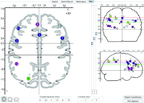
Nodes for S1 similarity subsets are illustrated in standard views provided by BrainMap Search&View. The S1 similarity subset (1,2,7,11; dark blue) best matched maximal cliques. The largest S1 similarity subset (4,5,8,9,12,13; violet) consists of mostly left, inferior, and anterior nodes, and the smallest S1 similarity subset (3,6,10; green) has the greatest A–P extent. Nodes are depicted graphically not according to their ALE volumes.

ALE‐P05 data

The number and size of nodes increased for the ALE‐P05 data and some nodes in the P05 data were made up of two nodes from the P01 data. This complicated the use of numbers to indicate results for the P05 data. P05‐to‐P01 number correspondence was found for all nodes but 5 and 12 of the 13‐node P01 data. The additional nodes 14–22 of the ALE‐P05 data had no corresponding nodes in the P01 data. ALE‐P05 results in Table IV use equivalent P01 numbering for nodes 1–13.

RDNA.

The first ALE‐P05 maximal clique was substantially different from the first ALE‐P01 maximal clique. However. it did contain three nodes common to the second ALE‐P01 maximal clique, nodes 1, 2, and 7, and was consistent with the five‐node dominant network reported by Neumann et al. [2005]. Beyond the first maximal clique, no clear relationship was seen with other ALE‐P01 cliques.

FSNA.

Changes in S1 and S2 subsets with changing ALE threshold were more predictable, with some changes seen as new nodes appended to existing subsets. For example, the (1,2,7,11) S1 subset from the ALE‐P01 data falls within the (1,2,7,11,19,21) S1 subset of the ALE‐P05 data. The additional node 19 (light blue, Fig. 3) seems to be a right side equivalent of node 11, both in middle frontal gyrus and in BA9. The additional node 21 was in putamen. Other S1 subsets formed into various groups with the additional nodes 14–22. As seen with the ALE‐P01 data, S1 subsets of the ALE‐P05 data can be formed from combinations of its S2 subsets.

Experiment Clustering

As was seen with node clustering, FSNA S2 similarity produced more and generally smaller subsets than S1 similarity (Table V, column 1). Unlike that with node clustering, S2 experiment subsets do not seem to be subgroups of S1 subsets. Thresholds used for experiment clustering were the same as used for node clustering. Two experiments (4 and 9) did not appear in the S2 subsets because these experiments reported no activations within the ALE VOIs used in generating the experiment table, and were not relevant for S2 similarity.

Table V.

Profile of experiment subsets for pooled ALE‐P01 Stroop meta‐analysis

Experiment subset	Control				Response		Modality			Statistic
	Congruent	Neutral	Nonlexical	Combo	Verbal	Manual	PET	Block fMRI	ER fMRI	(t,z)	Other
S1 Similarity
3,5,6,8,13,16,19	0.526	0.474	0.526	0.737	0.474	0.526	0.526	0.526	0.579	0.421	0.579
1,2,4,9,11,14,15,17,18	0.526	0.474	0.632	0.421	0.579	0.421	0.632	0.0421	0.474	0.526	0.474
7,10,12	0.421	0.789	0.737	0.737	0.263	0.737	0.526	0.632	0.684	0.316	0.684
S2 Similarity
3,8,16	0.632	0.579	0.737	0.737	0.474	0.526	0.737	0.421	0.684	0.316	0.684
5,13,14,19	0.474	0.632	0.684	0.789	0.211	0.789	0.474	0.684	0.632	0.368	0.632
2,7,10,12	0.474	0.737	0.684	0.684	0.316	0.684	0.579	0.579	0.632	0.368	0.632
1,6,11,15,17,18	0.368	0.526	0.789	0.684	0.526	0.474	0.579	0.474	0.632	0.474	0.526

Boldface type indicates highest similarity by subset in each of the four profile categories.

A nice feature of binary similarity coefficients is that they can also be used to compare experiment subsets with experiment factors of interest. For the ALE P01 data, this comparison was based on similarity between pairs of 19‐element binary patterns, one for experiment subsets and one for experiment factors. Setting bit values to 1 for the experiments in the similarity subset and 0 otherwise forms a 19‐element binary pattern for each experiment subset. A similar set of binary patterns can be formed for each experiment factor. Eleven experiment factors were grouped into four categories for the comparison (Table V). The largest similarity fractions provide an indication of which factor in each category best relates to each experiment subset. Paired (control, response) profiles, based on largest response similarity, were either (neutral, manual), (nonlexical, verbal), or (combination, verbal). The (nonlexical, verbal) S1 similarity profile favored positron emission tomography (PET) as the modality and t, z as the statistic, and the other two S1 profiles favored event‐related (ER) fMRI as the modality and a statistical approach other than t, z. These findings generally were consistent with visual inspection of the experiment summary in Table III. S2 similarity often had conflicts with the S1 similarity analysis and therefore was not considered appropriate for experiment analysis. This conflict seems mediated by the fact that S2 similarity does not consider absence as relevant.

A comprehensive node‐to‐experiment profile can be calculated using all nodes from the pooled ALE‐P01 data. For this profile study, 19‐element experiment patterns for each node from the experiment table are compared to 19‐element experiment factor patterns. As such, this profile does not depend on clustering by either RDNA or FSNA. Similarity between nodes and experiment factors is then measured using the S1 similarity coefficient.

A review of Table VI shows the highest mean similarity for control type was for experiments using nonlexical and combination controls. This was followed by neutral and finally by congruent, which had the lowest relationship across nodes. These observations are consistent with the claim that nonlexical and combination controls are preferred over the congruent control, due to the higher attentional requirements of the congruent condition [Milham et al.,2002].

Experiments using manual response had the highest similarity with node 2 (left inferior frontal gyrus, BA9) and node 6 (left precuneus, BA7). Experiments using verbal response had the highest similarity with node 5 (left inferior frontal gyrus, BA44). These response‐to‐node relationships, based only on ranking of similarity coefficients from the pooled Stroop meta‐analysis data, are consistent with findings from the more detailed verbal and manual Stroop meta‐analyses reported in Table V of Laird et al. [2005a].

Several additional factors were included in the Table VI profile to determine P value and group size effects. Mean similarity across nodes increased as the experiment P value changed from the all P < 0.05 to the all P < 0.001. This was anticipated because the largest variety of experiments (19) were included in the all P < 0.05. The all P < 0.005 included 11 experiments, whereas the all P < 0.001 had only two experiments. The two experiments in this latter group (Experiments 1 and 3) were indeed similar across tested factors, differing only by control type (Table III). A strong group‐size effect was seen, with the largest group studies (n > 20 subjects) showing the highest indices of similarity and with similarity diminishing with diminishing group size. This finding is consistent with the assumption that studies with larger numbers of subjects replicate better than do smaller group subject studies.

DISCUSSION

RDNA

The replicator dynamics method for determining a maximal clique was extended to find additional cliques for meta‐analysis networks. The importance of this capability was seen for the ALE‐P01 data where RDNA determined a two‐node first maximal clique (1,2) (Table IV). This two‐node outcome could have easily been predicted from Table II where nodes 1 and 2 are seen to have significantly higher incidences. If replicator dynamics only report this maximal clique, little would be gained from the analysis. The second maximal clique from the ALE‐P01 data was similar to the first maximal clique from the ALE‐P05 data, and both were consistent with the dominant network reported by Neumann et al. [2005], who used an ALE‐P05 type threshold but differing numbers of experiments and nodes. This finding shows that important cliques exist in a meta‐analysis network and can be found beyond the first using the recursive algorithm of RDNA. Determination of the first maximal clique by RDNA in the ALE‐P05 data benefited from having more and larger nodes. This was due partly to the more uniform distribution of node incidence, where the dispersion in node incidence (relative standard deviation) in the first six nodes dropped from 0.52 for ALE‐P01 data to 0.35 for ALE‐P05 data.

The node weights [Neumann et al.,2005] assigned by replicator dynamics to the (1,2) maximal clique summed to 0.944 rather than to the target value of 1.000. We noted that nodes 6, 7, and 11 accounted for almost all of the residual weight (0.0549), but that each node weight was too small to be clustered with the first maximal clique using the clustering threshold of 1/n = 1/13 = 0.077. The summed weights of the other three ALE‐P01 cliques in Table IV were all greater than 0.99. If the node‐clustering strategy had been to add moderate‐weight nodes to the clique until the summed weight exceeded 0.99, then the first maximal clique for the PO1 data would have been (1,2,6,7,11) rather than (1,2). This strategy seems reasonable because node weights beyond the additional three were several orders of magnitude smaller. Because there were more nodes in the ALE‐P05 data, the clustering threshold was smaller (1/22 = 0.045), and this was partly responsible for more nodes in the first maximal clique in that data. The above‐suggested node‐clustering strategy should avoid the problem mentioned in the theory section, that a clique determined using a 1/n threshold might be a subset of the maximal clique. The proposed summed node‐weight approach has not yet been evaluated, but this clustering method will be added to the RDNA software and testing carried out to determine its capabilities.

Although the significance of additional cliques is not clear in this study, it is believed that important network information can be found among those cliques. Maximal cliques are determined by maximizing co‐occurrence [Neumann et al.,2005], and this is reflected by the order in which they are determined by RDNA. Dominance within the overall network structure therefore is expected to follow maximal clique order, and this is useful information that is not provided by FSNA.

FSNA

In the context of analyzing a single study, failure to find activation is usually regarded as noninformative. In a meta‐analytic setting, the hierarchical structure of the observation model, induced by having many studies, renders informative the frequency of not reporting activations. This information is exploited by the S1 similarity measure and ignored in the S3 measure. Of the three similarity coefficients evaluated, S1 provided the greatest utility in analysis of meta‐analysis networks. It was used to formulate node subsets (Table IV), experiment subsets (Table V), and node‐to‐experiment profiles (Table VI). The Jaccard or S2 similarity was intermediate in binary pattern‐matching capability as it retained 1–0 and 0–1 mismatches in its formula. S2 similarity provided finer subdivisions of the S1 similarity node subsets, which add to the attractiveness the FSNA network‐processing tool. It was not seen to be useful in the analysis of experiment subsets. The S3 similarity coefficient failed to form multiple node or experiment subsets for data from the Stroop meta‐analysis. S3 similarity ignores the 1–0, 0–1, and 0–0 binary pairs when carrying out pattern analysis and therefore led to the smallest similarity coefficients. The high incidence of nodes 1 and 2 dominated S3 similarity, causing all other nodes to be maximally associated with these two nodes, masking other associations, and leading to a single subset. S3 similarity coefficients therefore were not deemed appropriate for forming subsets of nodes or experiments; however, co‐occurrence, which is linearly related to the S3 similarity coefficient, was well suited for analysis by RDNA.

Unlike RDNA, FSNA performed well with both ALE threshold data sets. Because we only detailed APE‐P01 data in tables, explanation of FSNA results focused on that data. An important result was that several key node relationships, only seen using separate verbal and manual ALE Stroop meta‐analyses [Laird et al.,2005a], were found using just the pooled data from the ALE‐P01 Stroop meta‐analysis. Achievement of this level of detail without extensive reanalysis is a very attractive feature of FSNA. The ability of FSNA to form subsets of experiments distinguishes it from RDNA, which was designed for network node analysis only. The information in profile tables such as Table V provide the researcher a means to rapidly review factors that best relate to the naturally determined experiment subsets. The S1 similarity of FSNA was also used to form the overall ALE node profile as seen in Table VI. The large feature set provided by FSNA make it a very attractive new tool for automated analysis of meta‐analysis networks.

Meta‐Analysis Networks

ALE determines a collection of brain VOIs that form a meta‐analysis network, and RDNA and FSNA enhance this data with special subsets. However, these analysis tools do not provide details of internodal connectivity. For example, in a coherently activated three‐node network there are four possible node‐link configurations, one a maximal clique (lower right, Fig. 4). The co‐occurrence matrix, which serves as the basis for RDNA, has the ability to encode these four configurations. Co‐occurrence values derived from a meta‐analysis network experiment table will encode a three‐node clique regardless of the node‐link configuration. The problem reported by Lohmann and Bohn [2002] with the other three node‐link configurations is avoided because the co‐occurrence network cannot encode them. Not surprisingly, RDNA returns (1,2,3) as the maximal clique for this network. The point is that all co‐active nodes in a meta‐analysis network are cliques. We expanded on this point by assuming that the co‐occurrence matrix for a meta‐analysis network is a summation of co‐occurrences from its constituent cliques. This is the basis for the recursive algorithm used by RDNA to determine multiple cliques in a meta‐analysis network.

Figure 4.

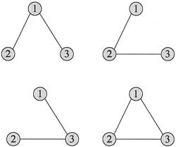
Four possible internodal configurations of a coherently activated 3‐node network.

The inability to encode connectivity becomes more serious as the number of nodes in a network increases. In the context of functional imaging studies, coherently activated nodes are active within the image acquisition time interval, and the order or duration of activations is not known. Event‐related potential (ERP) experiments with temporal resolution sufficient to determine the sequence of activated nodes could be helpful in resolving node‐link configurations. In addition, the ability of TMS to temporarily disable network nodes and observe the remainder of the network could be helpful for resolving node‐link configuration. With this additional information, the co‐occurrence matrix could be formulated more accurately and perhaps more meaningful subnetworks determined.

In functional imaging studies, experiments are defined based on control and test conditions and response type. Statistical parametric images are formed to investigate the system‐level network differences between fixed control and varying test conditions. A different contrast strategy was seen for Stroop functional imaging studies, where the incongruent test condition was contrasted with either neutral, congruent, nonlexical, or a mixture of control conditions, i.e., the control condition was varied rather than the test condition. The former approach investigates distributed neural networks relative to a fixed control state, whereas the latter approach investigates networks relative to a fixed test state. These differences should be emphasized when reporting findings. Moreover, for Stroop meta‐analysis two response types of were seen: verbal and manual; therefore, there were eight possible network configurations (four controls × two responses) for the Stroop meta‐analysis. The S1 similarity profile by experiments (Table V) indicated three dominant groupings of control–response profiles for the ALE‐P01: (neutral, manual), (nonlexical, verbal), and (combination, verbal) simplifying organization of findings.

Meta‐Analytic Functional Connectivity and Beyond

Functional connectivity is a statistical dependency between responses in one part of the brain and another. Usually, this dependency is assessed in terms of within‐subject correlations, but occasionally these dependencies are determined from correlations over subjects within a study. The co‐occurrence of activations among nodes of a meta‐analytic network harnesses exactly the same statistical dependency to infer functional connectivity among the nodes using correlations or similarities over studies. In this sense, the meta‐analysis networks are linked conceptually to the functional connectivity networks defined at a study and subject level. In the context of meta‐analysis networks, the source of variation inducing these dependencies are subtle changes in experimental design that can be characterized in terms of the statistical dependencies over experiments.

Although automated analysis tools for meta‐analysis networks are useful to determine network subsets that associate with contrasted conditions, they do not assess node activation levels or strength of internodal links. These tools provide an excellent framework for analysis of internodal interactions using other processing strategies such as structural equation modeling [Horowitz et al.,1999; McIntosh et al.,1994] and dynamic causal modeling [Friston et al.,2003].

CONCLUSIONS

Findings of the Stroop meta‐analysis using RDNA and FSNA generally were consistent with those obtained manually. RDNA provides a means to assess relative activity of networks, which helps to gauge the importance of network findings by both RDNA and FSNA. FSNA revealed details within the pooled meta‐analysis data that required multiple highly filtered meta‐analysis data sets when processed manually. S1‐ and S2‐type similarity together provide a hierarchical view of node associations. S3‐type similarity failed to form multiple subsets and was judged unsatisfactory. FSNA provides a more comprehensive meta‐analysis assessment than RDNA does, with tables for node similarity subsets, experiment similarity subsets, and overall node‐to‐factors similarity.

REFERENCES

- Anderberg MR (1973): Cluster analysis for applications. New York: Academic Press. [Google Scholar]
- Bomze IM, Pelillo M (2000): Approximating the maximum weight clique using replicator dynamics. IEEE Trans Neural Netw 11: 1228–1241. [DOI] [PubMed] [Google Scholar]
- Bower JM, Beeman D (1998): The book of GENESIS: exploring realistic neural models with the GEneral NEural SImulation System (2nd ed.). New York: Springer‐Verlag. [Google Scholar]
- Fox PT, Lancaster JL (2002): Mapping context and content: the BrainMap model. Nat Rev Neurosci 3: 319–321. [DOI] [PubMed] [Google Scholar]
- Friston KJ, Harrison L, Penny W (2003): Dynamic causal modeling. Neuroimage 19: 1273–1302. [DOI] [PubMed] [Google Scholar]
- Gardiner EJ, Artymiuk PJ, Willett P (1998): Clique‐detection algorithms for matching three‐dimensional molecular structures. J Mol Graph Model 15: 245–253. [DOI] [PubMed] [Google Scholar]
- Horowitz B, Tagamets MA, McIntosh AR (1999): Neural modeling, functional brain imaging, and cognition. Trends Cogn Sci 3: 91–98. [DOI] [PubMed] [Google Scholar]
- Johnson RA, Wichern DW (1988): Applied multivariate statistical analysis (2nd edition). Englewood Cliffs, NJ: Prentice Hall. [Google Scholar]
- Laird AR, McMillan KM, Lancaster JL, Kochunov P, Turkeltaub PE, Pardo JV, Fox PT (2005a): A comparison of label‐based review and activation likelihood estimation in the Stroop task. Human Brain Mapping 25: 6–21. [DOI] [PMC free article] [PubMed] [Google Scholar]
- Laird AR, Fox PM, Price CJ, Glahn DC, Uecker AM, Lancaster JL, Turkeltaub PE, Kochunov P, Fox PT. (2005b): ALE meta‐analysis: controlling the false discovery rate and performing statistical contrasts. Hum Brain Mapp 25: 155–164. [DOI] [PMC free article] [PubMed] [Google Scholar]
- Lancaster JL, Woldorff MG, Parsons LM, Liotti M, Freitas CS, Rainey L, Kochunov PV, Nickerson D, Mikiten SA, Fox PT (2000): Automated Talairach atlas labels for functional brain mapping. Hum Brain Mapp 10: 120–131. [DOI] [PMC free article] [PubMed] [Google Scholar]
- Lohmann G, Bohn S (2002): Using replicator dynamics for analyzing fMRI data of the human brain. IEEE Trans Med Imaging 21: 485–492. [DOI] [PubMed] [Google Scholar]
- Milham MP, Erickson KI, Banich MT, Kramer AF, Webb A, Wszalek T, Cohen NJ. (2002): Attentional control in the aging brain: insights from an fMRI study of the Stroop task. Brain Cogn 49: 277–296. [DOI] [PubMed] [Google Scholar]
- McIntosh AR, Grady CL, Ungerleider, Haxby JV, Rapoport SI, Horowitz B (1994): Network analysis of cortical visual pathways mapped with PET. J Neurosci 14: 656–666. [DOI] [PMC free article] [PubMed] [Google Scholar]
- Neumann J, Lohmann G, Derrfuss J, von Cramon DY (2005): The meta‐analysis of functional imaging data using replicator dynamics. Hum Brain Mapp 25: 165–173. [DOI] [PMC free article] [PubMed] [Google Scholar]
- Pelillo M, Siddiqi K, Zucker SW (1999): Matching hierarchical structures using association graphs. IEEE Trans Pattern Anal Mach Intell 21: 1105–1119. [Google Scholar]
- Samudrala R, Moult J (1998): A graph‐theoretic algorithm for comparative modeling of protein structure. J Mol Biol 279: 287–302. [DOI] [PubMed] [Google Scholar]
- Turkeltaub PE, Eden GF, Jones KM, Zeffiro TA (2002): Meta‐analysis of the functional neuroanatomy of single‐word reading: methods and validation. Neuroimage 16: 765–780. [DOI] [PubMed] [Google Scholar]