Genetic components of functional connectivity in the brain: The heritability of synchronization likelihood

Abstract

Cognitive functions require the integrated activity of multiple specialized, distributed brain areas. Such functional coupling depends on the existence of anatomical connections between the various brain areas as well as physiological processes whereby the activity in one area influences the activity in another area. Recently, the Synchronization Likelihood (SL) method was developed as a general method to study both linear and nonlinear aspects of coupling. In the present study the genetic architecture of the SL in different frequency bands was investigated. Using a large genetically informative sample of 569 subjects from 282 extended twin families we found that the SL is moderately to highly heritable (41–67%) especially in the alpha frequency (8–13 Hz) range. This index of functional connectivity of the brain has been associated with a number of pathological states of the brain. The significant heritability found here suggests that SL can be used to examine the genetic susceptibility to these conditions. Hum Brain Mapp, 2005. © 2005 Wiley‐Liss, Inc.

INTRODUCTION

Cognitive functions require the integrated activity of multiple specialized, distributed brain areas. Such functional coupling depends on the existence of anatomical connections between various brain areas as well as physiological processes whereby the activity in one area influences activity in another area. It is widely assumed that correlations between time series of activity of different brain areas reflect, to some extent, the functional interactions between these brain areas. For this reason, correlations between electroencephalography (EEG), magnetoencephalography (MEG), or blood oxygen level‐dependent (BOLD) signals from different brain regions are considered measures of “functional connectivity” [Lee et al., 2003]. Advanced statistical analysis allows inferring causal interactions from such time series, which is indicated by the concept of “effective connectivity” [Friston, 2002].

EEG and MEG have a relatively high time resolution, which makes these techniques suitable to study functional connectivity. The classic approach to determine statistical interdependencies between EEG signals is coherence, which is a measure of the linear correlation as a function of frequency [Nunez et al., 1997]. An alternative, more general approach to study functional connectivity is based on measures derived from dynamical systems theory [for an overview, see David et al., 2005; Quian Quiroga et al., 2002]. One of these measures is the synchronization likelihood (SL) [Stam and van Dijk, 2002]. The SL has been shown to be indicative of changes in functional connectivity during cognitive tasks [Micheloyannis et al., 2003; Stam et al., 2002a]. A reduced synchronization likelihood has been linked to degenerative disease [Babiloni et al., 2004; Pijnenburg et al., 2004; Stam et al., 2003a], whereas an increased synchronization likelihood is observed during epileptic seizures [Altenburg et al., 2003; Ferri et al., 2004]. In one study, SL analysis demonstrated differences between Alzheimer patients and healthy controls, whereas coherence analysis of the same data showed only a nonsignificant trend in the same direction [Stam et al., 2002b]. In another study it was shown that both MEG and EEG recordings are characterized by significant nonlinear correlations between the signals recorded from different brain regions [Stam et al., 2003a].

In view of the usefulness of SL as a general method to study changes in functional connectivity during cognitive processing and as a result of neurological disease, it is important to gain a better understanding of the factors that determine synchronization of the resting EEG. Although a number of studies have addressed genetic influences on individual differences in resting EEG measures, including coherence [for a meta‐analysis, see van Beijsterveldt and van Baal, 2002; for reviews, see van Beijsterveldt and Boomsma. 1994; Vogel, 2000], no studies have previously investigated the genetic architecture of SL. As a straightforward hypothesis we postulate here that the functional brain connectivity at rest as assessed by SL analysis depends largely on the genetically determined architecture of connected networks in the brain.

In the present study SL was determined in EEG recordings from 569 subjects who were all part of a monozygotic (MZ) twin pair, a dizygotic (DZ) twin pair, or who were nontwin siblings of these twins. Such a genetically informative design allows determination of the extent of interindividual differences in SL that can be ascribed to genetic differences or environmental differences [Boomsma et al., 2002; Martin et al., 1997]. The use of the so‐called extended twin design which includes twins as well as their singleton siblings ensures relative high statistical power to detect sources of environmental variation, and also boosts power to distinguish between variation due to genetic sources or due to environmental sources [Posthuma and Boomsma, 2000].

SUBJECTS AND METHODS

Subjects

Seven hundred ninety‐three healthy adult family members from 317 extended twin families participated in a study on the genetics of adult brain function [Posthuma, 2002] in which data on IQ scores, reaction times, and EEG recordings were obtained. All participants were obtained from the Netherlands Twin Registry [Boomsma, 1998]. Zygosity for same‐sex pairs was determined by typing highly polymorphic genetic markers (76% of the sample) or by means of questionnaire (24%). The complete sample consisted of two age cohorts: a young adult cohort with a mean of 26.2 years of age (SD 4.14) and an older adult cohort with a mean around 49.5 years of age (SD 7.14). Participating families consisted of one to eight siblings (including twins). On average, 2.5 offspring per family participated. In the young cohort 192 males and 213 females participated, in the older cohort 156 males and 232 females. Twenty‐eight subjects completed only the IQ test, but not the EEG recordings; thus, for 765 subjects EEG recordings were available. We decided to restrict our analyses to those persons for whom flawless recording was available at all electrode sites. This resulted in a total of 569 individuals (329 females) from 282 families for whom SL measures were calculated. The final young cohort included 38 MZ pairs, 49 DZ pairs, 53 single twins, and 79 additional siblings. The older cohort included 38 MZ pairs, 39 DZ pairs, 53 single twins, and 56 additional siblings.

The protocol of the study was approved by the scientific and medical‐ethical Review Board of Vrije Universiteit, Amsterdam. All subjects gave written informed consent after the nature of the procedure was explained. Subjects received a small financial bonus for participation.

EEG Recording

Three minutes of resting EEG was recorded while participants sat with their eyes closed in a dimly lit, sound‐attenuated, and electrically shielded cabin. The EEG was recorded with Ag/AgCl electrodes mounted in an electrocap. Signal registration was conducted using an AD amplifier developed by Twente Medical Systems (Enschede, The Netherlands) for 481 subjects or using NeuroScan 4.1 hardware (88 subjects). EEG signals were continuously represented online on a Nec multisync 17‐inch computer screen using POLY 5.0 software (POLY, 1999) or NeuroScan software and stored for offline processing. Standard 10–20 positions used were F7, F3, Fz, F4, F8, T3, C3, Cz, C4, T4, T5, P3, Pz, P4, T6, O1, and O2 [Jasper, 1958; Pivik et al., 1996]. Software‐linked earlobes (A1 and A2) served as references. The vertical electro‐oculogram (EOG) was recorded bipolarly between two Ag/AgCl electrodes, affixed 1 cm below the right eye and 1 cm above the eyebrow of the right eye. The horizontal EOG was recorded bipolarly between two Ag/AgCl electrodes affixed 1 cm left from the left eye and 1 cm right from the right eye. An Ag/AgCl electrode placed on the forehead was used as a ground electrode. Impedances of all EEG electrodes were kept below 3 kΩ, and impedances of the EOG electrodes were kept below 10 kΩ. The EEG was amplified poly (bandpass 0.05–30 Hz POLY; lowpass 50 Hz NeuroScan), digitized at 250 Hz, and stored for offline processing. Offline artifact‐free epochs of 4,096 samples (16.380 s) were selected for computation of the SL. An average reference was used (which included all electrodes except A1 and A2). EEG was digitally filtered offline in the delta (0.5–4 Hz), theta (4–8 Hz), alpha 1 (8–10 Hz), alpha 2 (10–13 Hz), or beta (13–30 Hz) bands. Digital filtering was done by applying a digital Fourier transform to the data, setting the real and imaginary components outside the bandpass to zero, and then applying an inverse Fourier transform to obtain the filtered time series. This approach does not induce phase shifts and has infinite steepness.

Determination of Synchronization Likelihood

The level of functional connectivity in the EEG was quantified with SL. SL is a measure of the statistical interdependencies between two time series, for instance, two EEG channels. SL takes on values between P_ref (a small number close to 0) in the case of independent time series and 1 in the case of fully synchronized time series. SL is sensitive to linear as well as nonlinear interdependencies and can be computed as a function of time, making it suitable for tracking time‐dependent changes at the synchronization level. For a technical description of the method and its properties, see Stam and van Dijk [2002], or the Appendix, in which the mathematical details are explained. A more intuitive explanation of the method is given in Figure 1.

Figure 1.

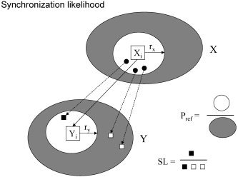
Schematic explanation of the synchronization likelihood. The gray areas X and Y represent the attractors of system X and Y. These attractors consist of a number of vectors X_i and Y_i which represent all possible states of system X and Y. The vectors are reconstructed from the time series by the procedure of time delay embedding. The synchronization likelihood (SL) between X and Y at time i is determined by considering all vectors in X that are closer to X_i than a critical distance r_x. These close neighbors of X_i are indicated by the white area around Xi. Each of these close neighbors of X_i (the three black dots in the white area) has a corresponding point (that is: a vector with the same time index) in Y: these are indicated by the black and white squares in Y. Some of these corresponding vectors in Y will be close to Y_i (the black square within the white area around Y_i, determined by r_y), others (the white squares, in the gray area) not. The SL is now defined as the likelihood that the corresponding vectors (the squares) will be close to Y_i (fall in the whiter area around Y_i). This likelihood is 1 in the case of perfect synchronization, and small in the case of no coupling. The value of the SL in the case of no coupling can be controlled by the use of P_ref, considering that in the case of no coupling the distribution of the squares over Y will be random. This is done by choosing the critical distances r_x and r_y such that the likelihood that a randomly chosen point in X will be closer to X than r_x equals P_ref; similarly, the likelihood that a random vector in Y will be closer to Y_i than r_y equals P_ref. P_ref is the same for X and Y, but r_x and r_y usually are not the same.

Genetic Analyses

All genetic analyses were carried out using the statistical software package Mx [Neale et al., 2003]. Estimation of genetic parameters was obtained by normal theory maximum likelihood. As the sample size did not allow testing of variance components across the two age cohorts and two sexes, we regressed SL on age and sex and decomposed the residual variation in SL of the full dataset into three components: additive genetic variation (A), common environmental variation (C) shared by family members, and a nonshared, or unique environmental variation (E) [see, e.g., Falconer and Mackay, 1996]. Common environmental variation, by definition, included all environmental sources of variation that twins and siblings from the same family share. Nonshared environmental variation refers to the environmental variation that is unique for an individual and that is typically not shared with family members, and also includes measurement error. For dizygotic (DZ) twins (and sib pairs) similarity in common environmental influences was fixed at 100%, similarity of additive genetic influences at 50% (since DZ twins and sib pairs on average share 50% of their segregating genes), and no similarity in nonshared environmental influences. Since monozygotic (MZ) twins share all their genes, MZ twin similarities for both additive genetic and common environmental influences were fixed at 100%. Thus, the expectation for the total variance is A+C+E, the expectation for the covariance between MZ twins is A+C, and the expectation for DZ twins/sibpairs is 1/2A+C.

Heritability is calculated as the proportional contribution of genetic variation to the total, observed variation. Given its sample size, this study could on average detect hertitabilities (i.e., influences of A) of 40% and above when α was set at 0.01. Goodness of fit of the variance decomposition models and significance of estimated parameters was determined by likelihood ratio tests.

RESULTS

In Table I descriptive statistics of SL measured per electrode and per frequency band are given. The mean values of the SL in different frequency bands are of the same order as in a number of previous studies, and reflect the weak connectivity of eyes‐closed resting state EEG [Stam et al., 2002a, b, 2003a; Stam and de Bruin, 2004].

Table I.

Descriptive statistics of synchronization likelihoods across different bands and electrode positions

	C3	C4	Cz	F3	F4	F7	F8	Fz	O1	O2	P3	P4	P7	P8	Pz	T7	T8
Delta
Mean	0.0821	0.0782	0.0818	0.1145	0.1145	0.0953	0.0928	0.1233	0.1164	0.1125	0.1100	0.1066	0.0929	0.0961	0.0947	0.0780	0.0837
SD	0.0162	0.0155	0.0135	0.0333	0.0352	0.0214	0.0213	0.0358	0.0294	0.0313	0.0244	0.0247	0.0254	0.0263	0.0236	0.0183	0.0188
Sex dev.	−0.0005	−0.0006	−0.0034	−0.0029	−0.0045	−0.0032	−0.0007	−0.0036	−0.0011	0.0010	−0.0051	−0.0039	0.0019	0.0029	−0.0075	0.0006	0.0001
Age	0.0001	0.0002	0.0001	0.0003	0.0004	0.0001	0.0002	0.0002	0.0003	0.0004	0.0001	0.0002	0.0004	0.0003	0.0004	0.0003	0.0001
MZ	0.03	0.12	0.16	0.47	0.36	0.20	0.06	0.48	0.29	0.38	0.11	0.29	0.36	0.36	0.27	0.24	0.12
DZ	0.08	0.19	0.02	0.18	0.14	0.07	0.04	0.16	0.16	0.15	0.11	0.08	0.08	0.07	0.19	0.19	0.22
Theta
Mean	0.0872	0.0794	0.0865	0.1026	0.1013	0.0864	0.0856	0.1118	0.0923	0.0890	0.0928	0.0927	0.0845	0.0857	0.0855	0.0830	0.0895
SD	0.0189	0.0179	0.0243	0.0332	0.0330	0.0227	0.0224	0.0336	0.0279	0.0287	0.0202	0.0188	0.0228	0.0225	0.0207	0.0136	0.0128
Sex dev.	−0.0035	−0.0007	−0.0023	0.0025	0.0045	−0.0004	0.0009	0.0025	0.0090	0.0086	−0.0005	−0.0004	0.0063	0.0048	−0.0062	−0.0002	−0.0014
Age	0.0003	0.0004	0.0005	0.0006	0.0007	0.0003	0.0003	0.0007	0.0007	0.0008	0.0003	0.0003	0.0006	0.0005	0.0004	0.0002	0.0001
MZ	0.56	0.46	0.65	0.54	0.51	0.43	0.43	0.61	0.45	0.49	0.28	0.30	0.32	0.41	0.46	0.37	−0.02
DZ	0.10	0.08	0.15	0.11	0.10	0.09	0.01	0.11	0.14	0.14	−0.02	−0.02	0.01	0.04	0.26	−0.07	0.06
Alpha1
Mean	0.1147	0.1102	0.1252	0.1719	0.1718	0.1380	0.1325	0.1808	0.1438	0.1442	0.1234	0.1246	0.1230	0.1276	0.1113	0.0984	0.1029
SD	0.0417	0.0394	0.0495	0.0662	0.0646	0.0547	0.0533	0.0646	0.0559	0.0552	0.0395	0.0418	0.0422	0.0437	0.0384	0.0295	0.0238
Sex dev.	0.0043	0.0032	0.0072	0.0172	0.0152	0.0147	0.0131	0.0158	0.0159	0.0200	0.0037	0.0089	0.0079	0.0132	−0.0017	0.0041	−0.0027
Age	0.0000	0.0001	0.0001	−0.0001	−0.0001	−0.0002	−0.0001	−0.0001	0.0001	0.0001	0.0000	0.0000	0.0001	0.0000	0.0002	0.0000	−0.0001
MZ	0.65	0.51	0.58	0.69	0.68	0.63	0.67	0.69	0.69	0.47	0.49	0.45	0.55	0.61	0.44	0.33	0.33
DZ	0.06	0.00	0.16	0.24	0.23	0.29	0.27	0.24	0.21	0.25	0.30	0.21	0.11	0.19	0.22	0.17	0.09
Alpha2
Mean	0.1238	0.1126	0.1379	0.2039	0.2014	0.1667	0.1598	0.2107	0.1709	0.1774	0.1422	0.1467	0.1276	0.1372	0.1250	0.1117	0.1094
SD	0.0353	0.0314	0.0407	0.0596	0.0579	0.0524	0.0505	0.0579	0.0524	0.0544	0.0409	0.0435	0.0341	0.0376	0.0407	0.0296	0.0280
Sex dev.	0.0061	0.0018	0.0035	0.0026	0.0034	0.0045	0.0072	0.0033	0.0070	0.0059	0.0058	0.0044	0.0055	0.0073	0.0030	0.0039	0.0037
Age	−0.0007	−0.0004	−0.0008	−0.0015	−0.0014	−0.0012	−0.0011	−0.0015	−0.0010	−0.0011	−0.0007	−0.0007	−0.0006	−0.0008	−0.0004	−0.0005	−0.0005
MZ	0.50	0.51	0.50	0.61	0.60	0.64	0.59	0.62	0.61	0.59	0.48	0.59	0.57	0.54	0.44	0.51	0.21
DZ	0.09	0.25	0.14	0.25	0.26	0.28	0.29	0.25	0.33	0.29	0.22	0.27	0.13	0.18	0.24	0.14	0.12
Beta
Mean	0.0821	0.0797	0.0859	0.1113	0.1090	0.0908	0.0866	0.1185	0.1009	0.1022	0.0953	0.0953	0.0854	0.0890	0.0805	0.0737	0.0753
SD	0.0111	0.0114	0.0136	0.0241	0.0247	0.0153	0.0153	0.0243	0.0201	0.0204	0.0133	0.0141	0.0147	0.0138	0.0164	0.0128	0.0122
Sex dev.	−0.0012	0.0010	−0.0025	−0.0023	−0.0022	−0.0024	0.0008	−0.0019	0.0022	0.0026	−0.0014	−0.0020	0.0024	0.0014	−0.0071	0.0006	0.0025
Age	0.0001	0.0002	0.0002	0.0002	0.0003	0.0000	0.0001	0.0004	0.0003	0.0003	0.0002	0.0002	0.0003	0.0001	0.0004	0.0001	0.0001
MZ	0.49	0.46	0.62	0.45	0.48	0.34	0.36	0.46	0.39	0.37	0.41	0.33	0.52	0.54	0.67	0.43	0.41
DZ	0.15	0.21	0.24	0.09	0.09	0.22	0.22	0.15	0.31	0.30	0.24	0.25	0.06	0.13	0.45	0.20	0.13

Females: N = 329; males: N = 240; Total: N = 569. Mean refers to grand mean, and SD to the standard deviation of the grand mean. Sex dev, male deviation of grand mean; age, regression weight of age; MZ, Monozygotic twin correlation; DZ, average dizygotic twin, twin‐sib, or sib‐sib correlation.

Table I also includes twin and sibling correlations for SL. MZ correlations are generally twice as high as DZ or sib correlations, suggesting the presence of genetic variation in SL. This was formally tested using variance decomposition models including variation due to additive genetic influences (A), common environmental influences (C), and nonshared environmental influences (E). The goodness of fit indices of these variance decomposition models were tested against those of saturated models in which the variation was not decomposed. For SL at all electrodes across all frequency bands, ACE models did not result in a worsening of the fit as compared to saturated models.

Figure 2 shows the proportional contribution of A, C, and E to the observed variation in SL, as estimated in the ACE models. By using a likelihood ratio test we determined whether fixing parameter A, C, or both parameters to zero resulted in a significant deterioration in fit statistic. This showed the influence of C was insignificant throughout: it reached significance (P = 0.043) only once for electrode PZ in the beta frequency range, where it was estimated at 23%. Considering the large number of tests and the single occurrence, it is reasonable to say that common environmental influences do not contribute to individual differences in SL. Additive genetic influences, however, reached significance for nearly all electrodes across all frequency bands. The exception was SL in the delta range, where either all variation was due to nonshared environmental influences including measurement error (C3, C4, Cz, F7, F8, P4, P7, P8, T8) or where we could not distinguish between A and C (F3, F4, Fz, O1, O2, P3, Pz, T7). For most leads an AE model was found to be the most parsimonious. Under the AE model, the highest heritabilities were found in the alpha 1 band, ranging from 47–72%, with a mean of 60%, the alpha 2 band, ranging from 43–63% with a mean of 56%, and in the beta band ranging from 38–70%), with a mean of 49%. The mean heritability in the theta band as estimated from the AE model was 44% (ranging from 33–55%).

Figure 2.

Decomposition of the observed variance in SL across 17 different electrode positions (horizontal axis) for the five frequency bands delta, theta, alpha 1, alpha 2, and beta. The variance is decomposed into three sources: additive genetic influences (A, heritability), common environmental influences (C), and nonshared environmental influences (E). The vertical axis represents the percent of the total variance that is explained by each of the three sources. All values of A, C, and E are based on estimates from the model in which all three sources of variation were included. The dotted line indicates the contribution of additive genetic factors to SL variance that, on average, could be detected with a significance level of 0.01.

DISCUSSION

In view of the usefulness of SL as a general method to study changes in functional connectivity during cognitive processing and as a result of neurological disease [Altenburg et al., 2003; Babiloni et al., 2004; Bruin et al., 2004; Dumont et al., 2004; Ferri et al., 2004; Micheloyannis et al., 2003; Pijenburg et al., 2004; Stam, 2003, 2004; Stam and van Dijk, 2002; Stam et al., 2002a, b, 2003a, b; Stam and de Bruin, 2004], it seemed important to gain a better understanding of the factors that determine synchronization of the resting EEG. Specifically, we wanted to test the contribution of genetic factors to individual variance in this trait. Although a number of twin studies have addressed genetic influences on individual differences in other resting EEG measures, this is the first study that investigates the genetic architecture of SL. Using a large sample of 569 healthy adult subjects from 282 extended twin families, we found that SL is moderately to highly heritable (33–70%) especially in the alpha frequency range (8–13 Hz).

This adds SL to the list of statistical features of the resting EEG signal that depend on genetic factors. Previous twin studies have reported very high heritability estimates (between 70 and 80%) for alpha peak frequency in adults [Christian et al., 1996; Posthuma et al., 2001]. Van Beijsterveldt and van Baal [2002] conducted a meta‐analysis on adult EEG alpha power as measured in 11 relatively small‐scaled genetic studies. Although these studies were heterogeneous and did not provide a single estimate of heritability, van Beijsterveldt and van Baal concluded that variability in EEG alpha power is largely determined by genetic factors. Finally, a number of studies have examined the genetics of EEG‐coherence, which is the normalized cross‐correlation of the EEG signal at two different electrodes, and is suggested to index the degree of functional connectivity between brain areas underlying the two electrode sites. In a small sample of 5‐ and 6‐year‐old twins, Ibatoullina et al. [1994] found very low heritabilities for interhemispheric coherences. In contrast, van Baal et al. [1998] found substantial heritabilities (ranging from 37–75%) for coherence along the anterior/posterior axis within the theta frequency, using a dataset of 209 twin pairs aged 5. Van Baal et al., [2001] tested the same twin pairs again after 1.5 years. For frontal connections, the influence of genetic factors decreased, while the estimates of heritability of posterior connections increased [van Baal et al., 2001]. Van Beijsterveldt et al. [1998] performed a study in an adolescent group of 213 twin pairs and found an average heritability of EEG coherence of 60, 65, and 60% in the theta, alpha, and beta frequency bands, respectively.

Compared to coherence analysis, SL is an interesting alternative measure of functional connectivity because it is sensitive to linear as well as nonlinear aspects of coupling and can deal with nonstationarity. This added value is demonstrated, for instance, by the finding that differences between mildly demented Alzheimer patients and healthy controls can be demonstrated with SL analysis but not with coherence analysis of the same MEG data [Stam et al., 2002b]. Previously, we have shown that both MEG and EEG recordings in healthy subjects are characterized by moderate but highly significant nonlinear correlations between signals recorded from different brain regions, as well as nonstationary “itinerant” dynamics [Stam et al., 2003a]. This nonlinear element of functional connectivity is not considered a mere epiphenomenon. First, nonlinear correlations cannot be explained by volume conductions, and therefore are more likely to reflect true functional connectivity. Second, the nonstationary “itinerant” dynamics might reflect a fundamental aspect of information processing in the brain. This process of “fragile binding” is characterized by the rapid creation and destruction of functional cell assemblies [Friston, 2000; Breakspear et al., 2004]. SL therefore may more accurately reflect actual information processing between brain areas because of its sensitivity to nonlinear structure and suitability for nonstationary datasets.

Functional brain connectivity in the resting state is characterized by a default network which involves, among others, the posterior cingulate cortex, the hippocampus, frontal, and parietal association cortex. The importance of this resting state for cognition has recently been stressed by fMRI studies [Greicius et al., 2003, 2004]. Although EEG lacks the spatial resolution of fMRI, its high temporal resolution allows the analysis of nonstationary and nonlinear properties of this default network. In view of its predictive value for a number of pathological states [Altenburg et al., 2003; Babiloni et al., 2004; Ferri et al., 2004; Micheloyannis et al., 2003; Pijnenburg et al., 2004 Stam et al., 2002a, 2003a], we propose that, when searching for the actual genetic variation influencing these conditions, SL can serve as a valuable addition to the existing EEG endophenotypes.

Mathematical Background of Dynamical Systems Theory, Generalized Synchronization, and Synchronization Likelihood

Here we briefly recapture some basic notions from dynamical systems theory and give a formal definition of synchronization likelihood (SL). The key step is to reconstruct, from a time series of observations, the attractor of the underlying dynamical system.

Assume we have two time series x_i and y_i, where the index i, i = (1..N), denotes discrete time. From each of these time series we construct a series of m dimensional vectors X_i and Y_i in state space with the method of time‐delay embedding [Takens, 1981] as follows:

(1)

where L is the time lag, and m the embedding dimension (m ≪ N). From a time series of N samples, N–(m × L) vectors can be reconstructed. Takens has proven mathematically that, for a sufficiently high m, the reconstructed vectors correspond to the attractor of the underlying dynamical system [Takens, 1981]. The attractor is a geometric object in the state space (or phase space) of a dynamical system, which represents its fundamental characteristics such as its degrees of freedom, sensitive dependence on initial conditions and conservative or dissipative dynamics. The general equation for a dynamical system is:

(2)

Here μ represents a set of parameters and ϵ is noise. A dynamical system X is said to be linear if G is linear (system of linear differential equations), otherwise X is nonlinear. The attractor of the dynamical system is the geometric representation of the solution of the equations of motion. Interactions between two dynamical systems X and Y can be described by the concept of generalized synchronization, as introduced by Rulkov et al. [1994]:

(3)

This equation says that the state of dynamical system Y (the response system) is a function F of the state of dynamical system X (the driver system). The function F maps each point of X on a corresponding point of Y. The only requirement is that F is locally smooth. The coupling between X and Y is said to be linear when F is linear, and nonlinear if F is nonlinear.

The synchronization likelihood is an algorithm to determine the strength of generalized synchronization between two systems X and Y, where X and Y are obtained from time series by time delay embedding (Eq. 1). Since the method is based on what can be considered a local linear approximation of F, it can handle linear and well as nonlinear cases of F. The fundamental idea is that two points on X that are very close together should be mapped to two points on Y that are also very close together if Eq. 3 holds.

Synchronization likelihood is defined as the conditional likelihood that the distance between Y_i and Y_j will be smaller than a cutoff distance r_y, given that the distance between X_i and X_j is smaller than a cutoff distance r_x. In the case of maximal synchronization this likelihood is 1; in the case of independent systems, it is a small, but nonzero number, namely, P_ref. This small number is the likelihood that two randomly chosen vectors Y (or X) will be closer than the cutoff distance r. In practice, the cut‐off distance is chosen such that the likelihood of random vectors being close is fixed at P_ref, which is chosen the same for X and for Y. To understand how P_ref is used to fix r_x and r_y we first consider the correlation integral:

(4)

Here the correlation integral C_r is the likelihood that two randomly chosen vectors X will be closer than r. The vertical bars represent the Euclidean distance between the vectors. N is the number of vectors, w is the Theiler correction for autocorrelation (Theiler, 1986), and θ is the Heaviside function: θ(X) = 0 if X ≥ 0 and θ(X) = 1 if X < 0. Now, r_x is chosen such that Cr_x = P_ref and r_y is chosen such that Cr_y = P_ref. The synchronization likelihood between X and Y can now be formally defined as:

(5)

SL is a symmetric measure of the strength of synchronization between X and Y (SL_XY = SL_YX). In Eq. 5 the averaging is done over all i and j; by doing the averaging only over j, SL can be computed as a function of time i. From Eq. 5 it can be seen that in the case of complete synchronization SL = 1; in the case of complete independence SL = P_ref. In the case of intermediate levels of synchronization P_ref < SL < 1.

In the present study the parameters were set as follows: w1 = 100, lag L = 10; embedding dimension m = 10; P_ref = 0.05. These choices were the same as in a number of previous studies [Stam et al., 2002a, b, 2003b; Stam and de Bruin, 2004). We computed for each of the 17 channels the synchronization likelihood between that particular channel and all other channels. This approach was used to allow comparison between the present study and previous published studies using the synchronization likelihood in which a similar approach to averaging was taken.

REFERENCES

- Altenburg J, Vermeulen RJ, Strijers RLM, Fetter WPF, Stam CJ (2003): Seizure detection in the neonatal EEG with synchronization likelihood. Clin Neurophysiol 114: 50–55. [DOI] [PubMed] [Google Scholar]
- Babiloni C, Ferri F, Moretti DV, Strambi A, Binetti G, Dal Forno G, Ferreri F, Lanuzza B, Bonato C, Nobili F, Rodriguez G, Salinari S, Passero S, Rocchi R, Stam CJ, Rossini PM (2004): Abnormal fronto‐parieto coupling of brain rhythms in mild Alzheimer's disease: a multicentric EEG study. Eur J Neurosci 19: 1–9. [DOI] [PubMed] [Google Scholar]
- Boomsma DI (1998): Twin registers in Europe: an overview. Twin Res 1: 34–51. [DOI] [PubMed] [Google Scholar]
- Boomsma D, Busjahn A, Peltonen L (2002): Classical twin studies and beyond. Nat Rev Genet 3: 872–882. [DOI] [PubMed] [Google Scholar]
- Breakspear M, Williams LM, Stam CJ (2004): A novel method for the topographic analysis of neural activity reveals formation and dissolution of ‘dynamic cell assemblies.’ J Computat Neurosci 16: 49–68. [DOI] [PubMed] [Google Scholar]
- de Bruin EA, Bijl S, Stam CJ, Bocker BE, Kenemans JL, Verbaten MN (2004): Abnormal EEG synchronisation in heavily drinking students. Clin Neurophysiol 115: 2048–2055. [DOI] [PubMed] [Google Scholar]
- Christian JC, Morzorati S, Norton JA Jr, Williams CJ, O'Connor S, Li TK (1996): Genetic analysis of the resting electroencephalographic power spectrum in human twins. Psychophysiology 33: 584–591. [DOI] [PubMed] [Google Scholar]
- David O, Cosmelli D, Friston KJ (2004): Evaluation of different measures of functional connectivity using a neural mass model. Neuroimage 21: 659–673. [DOI] [PubMed] [Google Scholar]
- Dumont M, Jurysta F, Lanquart J‐P, Migeotte P‐F, van de Borne P, Linkowski P (2004): Interdependency between heart rate variability and sleep EEG: linear/non‐linear? Clin Neurophysiol 115: 2031–2040. [DOI] [PubMed] [Google Scholar]
- Falconer DS, Mackay TFC (1996): Introduction to quantitative genetics, 4th ed. Harlow, UK: Longan Group. [Google Scholar]
- Ferri R, Stam CJ, Lanuzza B, Cosentino F, Elia M, Musumeci S, Pennisi G (2004): Different EEG frequency band synchronization during nocturnal frontal lobe seizures. Clin Neurophysiol 115: 1202–1211. [DOI] [PubMed] [Google Scholar]
- Friston KJ (2002): Functional integration and inference in the brain. Prog Neurobiol 68: 113–143. [DOI] [PubMed] [Google Scholar]
- Greicius MD, Krasnow B, Reiss AL, Menon V (2003): Functional connectivity in the resting brain: a netork analysis of the default mode hypothesis. Proc Natl Acad Sci U S A 100: 253–258. [DOI] [PMC free article] [PubMed] [Google Scholar]
- Greicius MD, Srivastava G, Reiss AL, Menon V (2004): Default‐mode network activity distinguishes Alzheimer's disease from heathy aging: evidence from functional MRI. Proc Natl Acad Sci U S A 101: 4637–4642. [DOI] [PMC free article] [PubMed] [Google Scholar]
- Ibatoullina A, Vardaris R, Thompson L (1994): Genetic and environmental influences on the coherence of background and orienting response EEG in children. Intelligence 19: 65–78. [Google Scholar]
- Lee K‐H, Williams LM, Breakspear M, Gordon E (2003): Synchronous gamma activity: a review and contribution to an integrative neuroscience model of schizophrenia. Brain Res Rev 41: 57–78. [DOI] [PubMed] [Google Scholar]
- Martin NG, Boomsma DI, Machin G (1997): A twin pronged attack on complex traits. Nat Genet 17: 387–392. [DOI] [PubMed] [Google Scholar]
- Micheloyannis S, Vourkas M, Bizas M, Simos P, Stam CJ (2003): Changes in linear and non‐linear EEG measures as a function of task complexity: evidence for local and distant signal synchronization. Brain Topogr 15: 239–247. [DOI] [PubMed] [Google Scholar]
- Neale MC, Boker SM, Xie G, Maes HH (1999): Mx: statistical modeling, 5th ed. Richmond VA: Department of Psychiatry. [Google Scholar]
- Nunez PL, Srinivasan R, Westdorp AF, Wijesinghe RS, Tucker DM, Silberstein RB, Cadusch PJ (1997): EEG coherency I: statistics, reference electrode, volume conduction, Laplacians, cortical imaging, and interpretation at multiple scales. Electroenceph Clin Neurophysiol 103: 499–515. [DOI] [PubMed] [Google Scholar]
- Pijnenburg YAL, van de Made Y, van Cappellen van Walsum, AM , Knol DL, Scheltens Ph, Stam CJ (2004): EEG synchronization likelihood in mild cognitive impairment and Alzheimer's disease during a working memory task. Clin Neurophysiol 115: 1332–1339. [DOI] [PubMed] [Google Scholar]
- Posthuma D (2002): Genetic variation and cognitive ability. PhD Thesis: Vrije Universiteit Amsterdam. Print Partners Ipskamp, Enschede.
- Posthuma D, Boomsma DI (2000): A note on the statistical power in extended twin designs. Behav Genet 30: 147–158. [DOI] [PubMed] [Google Scholar]
- Posthuma D, Boomsma DI, de Geus EJC (2001): Are smarter brains running faster? Heritability of alpha peak frequency, IQ and their interrelation. Behav Genet 31: 567–579. [DOI] [PubMed] [Google Scholar]
- Quian Quiroga R, Kraskov A, Kreuz T, Grassberger G (2002): Performance of different synchronization measures in real data: a case study on electroencephalographic signals. Phys Rev E 65: 041903. [DOI] [PubMed] [Google Scholar]
- Rulkov NF, Sushchik MM, Ysimring LS, Abarbanel HDI (1995): Generalized synchronization of chaos in directionally coupled chaotic systems. Phys Rev E 51: 980–994. [DOI] [PubMed] [Google Scholar]
- Stam CJ (2003): Chaos, continuous EEG, and cognitive mechanisms: a future for clinical neurophysiology. Am J END Technol 43: 1–17. [Google Scholar]
- Stam CJ (2004): Functional connectivity patterns of human magnetoencephalographic recordings: a “small‐world” network? Neurosci Lett 355: 25–28. [DOI] [PubMed] [Google Scholar]
- Stam CJ, de Bruin EA (2004): Scale‐free dynamics of global functional connectivity in the human brain. Hum Brain Mapp 22: 97–109. [DOI] [PMC free article] [PubMed] [Google Scholar]
- Stam CJ, van Dijk BW (2002): Synchronization likelihood: an unbiased measure of generalized synchronization in multivariate data sets. Physica D 163: 236–241. [Google Scholar]
- Stam CJ, van Cappellen van Walsum AM, Micheloyannis S (2002a): Variability of EEG synchronization during a working memory task in healthy subjects. Int J Psychophysiol 46: 53–66. [DOI] [PubMed] [Google Scholar]
- Stam CJ, van Cappellen van Walsum AM, Pijnenburg YAL, Berendse HW, de Munck JC, Scheltens Ph, van Dijk BW (2002b): Generalized synchronization of MEG recordings in Alzheimer's disease: evidence for involvement of the gamma band. J Clin Neurophysiol 19: 562–574. [DOI] [PubMed] [Google Scholar]
- Stam CJ, Breakspear M, van Cappellen van Walsum AM, van Dijk BW (2003a): Nonlinear synchronization in EEG and whole‐head MEG recordings of healthy subjects. Hum Brain Mapp 19: 63–78. [DOI] [PMC free article] [PubMed] [Google Scholar]
- Stam CJ, van der Made Y, Pijnenburg YAL, Scheltens PH (2003b): EEG synchronization in mild cognitive impairment and Alzheimer's disease. Acta Neurol Scand 108: 90–96. [DOI] [PubMed] [Google Scholar]
- Takens F (1981): Detecting strange attractors in turbulence. Lecture Notes Math 898: 366–381. [Google Scholar]
- Theiler J (1986): Spurious dimension from correlation algorithms applied to limited time‐series data. Phys Rev A 34: 2427–2432. [DOI] [PubMed] [Google Scholar]
- van Baal GCM, de Geus EJC, Boomsma DI (1996): Genetic architecture of EEG power spectra in early life. Electroencephalogr Clin Neurophysiol 98: 502–514. [DOI] [PubMed] [Google Scholar]
- van Beijsterveldt CEM, Boomsma DI (1994): Genetics of the human electroencephalogram (EEG) and event‐related brain potentials (ERPs): a review. Hum Genet 94: 319–330. [DOI] [PubMed] [Google Scholar]
- van Beijsterveldt CEM, van Baal GCM (2002): Causes of individual differences in the human electroencephalogram: a review and a meta‐analysis of twin and family studies. Biol Psychol 61: 11–38. [DOI] [PubMed] [Google Scholar]
- Vogel F (2000): Genetics and the electroencephalogram. Berlin: Springer. [Google Scholar]