Sparse imaging and continuous event‐related fMRI in the visual domain: A systematic comparison

Abstract

Continuous image acquisition as used in most functional magnetic resonance imaging (fMRI) designs may conflict with specific experimental settings due to attendant, noisy gradient switching. In sparse fMRI, single images are recorded with a delay that allows the registration of the predicted peak of an evoked hemodynamic response (HDR). The aim of this study was to assess validity and sensitivity of single‐trial sparse imaging within the visual domain. Thirteen subjects were scanned twice. Either continuous or sparse image acquisition was applied while participants viewed single trains of flashlights. Sparse fMRI results were compared to continuous event‐related fMRI results on single‐ and multisubject level regarding spatial extent, overlap, and intensity of activation. In continuously recorded data, the variability of the HDR peak latency was examined because this measure determined the timing of sparse image acquisition. In sparse fMRI, the sensitivity was analyzed considering different numbers of averaged trials. Sparse imaging detected the core activity revealed using continuous fMRI. The intensity of signal changes detected by continuous or sparse fMRI was comparable. The HDR peak latency was stable across sessions, but intersubject and regional variability might have affected the power of sparse fMRI. In sparse imaging, adding trials resulted in extension of activation and improvement in statistical power. The comparison with established continuous fMRI confirms the validity of sparse imaging. Conventional event‐related data acquisition and analysis provided more comprehensive results. However, only sparse fMRI offers the opportunity to apply stimuli and record further biosignals free of scanner‐related artifacts during intervals without image acquisition. Hum. Brain Mapping 24:130–143, 2005. © 2004 Wiley‐Liss, Inc.

INTRODUCTION

Sparse imaging describes an event‐related functional magnetic resonance imaging (fMRI) scheme containing defined times without image acquisition. Scanning is triggered several seconds after stimulus presentation, taking into account the physiologic delay of the hemodynamic response (HDR). The blood oxygenation level‐dependent (BOLD) response, a term established by Ogawa et al. [1990], significantly increases 2 s after stimulus presentation [Fransson et al., 1998], peaks after brief stimulation (2 s or less) after 5–6 s [Birn et al., 1999; Rosen et al., 1998; Savoy et al., 1995], and lasts approximately 10–12 s [Buckner, 1998]. Before the signal returns to baseline, an undershoot in its intensity is observed frequently [Friston et al., 1998]. In sparse fMRI experiments, images are sampled with a delay suitable to register the HDR evoked by the applied stimulus.

Until now, sparse fMRI techniques have been used primarily in the auditory domain. This method of image acquisition was developed mainly for practical reasons inherent in the nature of acoustic stimulus presentation. In a conventional blocked or event‐related design, the attendant gradient switching during image acquisition causes loud noise that masks acoustic stimuli and produces undesirable brain activation [Backes and van Dijk, 2002; Bandettini et al., 1998; Belin et al., 1999; Eden et al., 1999; Hall et al., 1999; MacSweeney et al., 2000; Müller et al., 2003; Yang et al., 2000]. To avoid this problem, fMRI designs have been devised that interrupt continuous scanning. Sparse imaging techniques imply time intervals without scanner activity, that is, without interference resulting from noisy gradient switching. Within these silent periods, tones, sounds, or speech stimuli can be delivered solely.

To minimize scanner noise effects on auditory cortex, various sparse imaging approaches have been developed. In a recent study by our group, single brain volumes were recorded time‐locked to the stimuli of interest to reveal a network of auditory target detection [Müller et al., 2003]. Separated by intervals of 10 heartbeats, Backes and van Dijk [2002] acquired single slices at various times of the BOLD response to capture activity in auditory cortex and brainstem induced by brief auditory stimuli. Belin et al. [1999] used a constant, unusually long interval between successive functional image acquisition, whereas auditory stimuli were presented at different delays before scanning occurred to reconstruct the shape of the HDR. However, this method does not completely exclude the possibility of scanner noise influencing auditory stimulus processing. If an auditory stimulus is presented long before the next volume acquisition, it is temporally close to the previous image acquisition. As a result, the BOLD response to the auditory stimulus is likely to be affected by that of the preceding acquisition‐induced noise. Eden et al. [1999] measured single brain volumes after an 8‐s period during which subjects carried out a motor task. They found performance‐related BOLD signal changes comparable to those derived using a blocked design. Participants of a study by Hall et al. [1999] listened to episodes of 14‐s duration while single brain volumes were recorded after the stimulation epochs and baseline conditions of equal length. The latter studies combine the idea of sparse temporal sampling with prolonged stimulus presentation. However, these approaches have limited temporal resolution, and may not be useful to isolate transient cognitive processes. Yang et al. [2000] carried out single‐trial sparse imaging of acoustically evoked activity and compared the results to three datasets of a typical event‐related functional image acquisition technique but did not find similar results. This finding is not surprising because the attendant noisy gradient switching during continuous image acquisition changed the experimental paradigm. It represents an additional, interfering source of acoustic stimulation producing auditory system stimulation [Backes and van Dijk, 2002; Belin et al., 1999; Eden et al., 1999; Hall et al., 1999; Yang et al., 2000], and it might have increased the difficulty of perceiving the applied tone bursts. Accordingly, sparse fMRI can be validated only outside the auditory domain.

The aim of the present study was to demonstrate the validity and efficiency of single‐trial sparse imaging within the visual domain. The visual system was chosen because visual stimuli are known to evoke a robust activation response [McFadzean et al., 1999]. A flicker paradigm, known to evoke primary visual cortex (Brodmann area [BA] 17) activation, was applied in this study [Janz et al., 2000; Miki et al., 2000]. Miezin et al. [2000] found stable HDR onsets, amplitudes, and times to peak for a given region within the same subjects across different imaging sessions, and stated strong central tendencies for these parameters when averaging across subjects. With respect to these results, the induced averaged (across participants) HDR regarding these parameters was expected to be robust for early visual cortex areas. We applied a single‐trial sparse fMRI scheme that aimed at registering only the stimulus‐induced HDR peak to obtain the maximal detectable contrast in comparison to reference trials. Imaging data were also collected in a comparable event‐related setting with continuous image acquisition and convolved with a canonical HDR reference function and its temporal derivative [Josephs et al., 1997]. In this manner, results of sparse fMRI could be compared systematically to that of an established imaging method. Indeed, it is known that acoustic scanner noise can indirectly confound fMRI results even in experiments within the visual modality. The scanning‐related noise during continuous fMRI may distract subjects and require them to enhance their mental effort to handle the experimental demands [Mazard et al., 2002; Moelker and Pattynama, 2003]. This effect is likely to increase with task difficulty [Elliott et al., 1999]. However, in the present study a paradigm that did not demand attentional effort was used; the comparison of noisy continuous event‐related with sparse fMRI for the purpose of validation of the latter is therefore admissible.

Comparisons of both imaging approaches were carried out on a single‐subject and on a group level. Averaged HDR peak latencies of successive imaging sessions were investigated with respect to variability across sessions and subjects, as stable and comparable HDR peak latencies (within a given region) benefit the sparse sampling approach. Finally, sparse imaging was subject to analyses on the effects of trial averaging to quantify alterations in spatial extent and statistical power depending on the number of trials. The advantage of sparse imaging over conventional continuous fMRI is that it offers the opportunity to apply stimuli and sample hemodynamic and further biosignal alterations, which are not affected by artifacts due to continuous scanner gradient switching.

SUBJECTS AND METHODS

Subjects

We assessed 13 healthy volunteers without neurologic or psychiatric disorders (four women, nine men; average age ± standard deviation [SD], 27.4 ± 4.6 years; age range, 21–40 years). All subjects were informed about the purpose of the study and gave their consent. The study protocol was approved by the local ethics committee.

Visual Stimulation

Visual stimuli were presented in real time using a standard PC with custom‐written software for stimulus presentation and synchronization of image acquisition. Visual stimuli or a red fixation point during rest periods were projected onto a white screen that could be seen via a head coil‐mounted mirror. Stimuli consisted of a series of 10 flashlights and were presented with a frequency of 5 Hz (stimulus duration = 2 s). We decided in favor of rather “long” brief events because Savoy et al. [1995] reported the amplitude of the HDR curve to increase with stimulus duration. During both continuous and sparse fMRI, a total of 45 visual stimuli were presented.

Data Acquisition

Each participant was scanned on two different days. During the first examination continuous event‐related data, whereas during the second examination sparse fMRI data were recorded. The fixed order of imaging designs should not have affected the results, as our paradigm did not demand higher cognitive processing and could be considered to be insensitive to learning effects.

Image data were acquired with a 1.5‐Tesla scanner (Sonata; Siemens Medical Solutions, Erlangen, Germany) utilizing a conventional head coil. When in the scanner, subjects lay supine with the head embedded in vacuum pads to minimize head movements. Headphones and earplugs were used to reduce the perception of scanner noise. Using a single‐shot T2*‐weighted echo‐planar imaging (EPI) sequence, 18 axial slices per volume were collected sequentially. Imaging parameters were: TA (acquisition time of a single volume) =1,800 ms; TE = 60 ms; flip angle = 90 degrees; field of view (FOV) = 230 mm; matrix size = 128 × 128 (interpolated), voxel size = 1.8 × 1.8 × 6.5 mm, slice thickness = 5 mm. Both sparse and continuous event‐related recordings were carried out using the same imaging sequence. In continuous scanning, TR equaled TA, whereas in sparse imaging the interstimulus interval determined TR.

Applying the continuous event‐related fMRI scheme, 600 images in total were recorded within three sessions. Subjects did not leave the scanner between sessions. Within each of these three sessions, 15 trains of flashlight stimuli (2 s each) were presented with variable onsets every 18 ± 3.6 s to optimize the HDR distribution estimation. The first five scans of each run were discarded to allow the magnetization to attain a steady state.

Sparse fMRI of a single brain volume started 4 s after stimulus onset (Fig. 1). The interscan interval was 25 s on average, ranging from 21–29 s to avoid periodicity of scans. To optimize the detection of BOLD signal changes induced by single‐trial presentation, we registered data in the peak period of the HDR curve. The latency of the HDR peak was determined by averaging the fitted data of the continuously acquired time series. The mean HDR peaked 5.13 ± 0.77 s after stimulus onset. Triggers inducing 1.8‐s long single volume acquisition were therefore programmed to be sent out 4 s after the beginning of each flashlight series. A total of 45 2‐s trains of flashlight stimuli were also presented during sparse fMRI within three successive sessions. Again, subjects did not leave the scanner between sessions. Within a single session, 15 volumes after visual stimulation and 15 images during a resting condition were acquired. In the latter condition, scanning was triggered without preceding stimulation. Stimulation and resting condition were alternated in a pseudorandomized manner.

Figure 1.

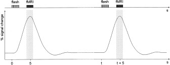
Schematic representation of the sparse acquisition scheme: fMRI of single brain volumes (TA = 1.8 s, TR = 21–29 s) started 4 s after presentation of 2‐s trains of 10 flashlight stimuli (5 Hz) to capture the peak period of the evoked HDR. The mean HDR peaked 5.13 s after stimulus onset.

Data Analysis

Imaging data were analyzed using the SPM99 software package (Wellcome Department of Cognitive Neurology, London, UK). In continuously acquired data, slice‐timing [Henson et al., 1999] was omitted because slices were acquired sequentially and the activation was concentrated on few slices. Timing differences were thus considered negligible, and preprocessing was identical for continuous and sparse fMRI data. For each participant, functional images were corrected for motion artifacts by a 3‐D rigid‐body realignment algorithm applying sinc interpolation, spatially normalized in reference to the Montréal Neurological Institute (MNI) template using bilinear interpolation, resliced with a voxel size of 2 × 2 × 2 mm, and subsequently smoothed with a Gaussian kernel of 9 mm full‐width at half‐maximum (FWHM). Statistical modeling and inference were based on the general linear model approach (GLM) [Friston et al., 1995].

HDRs recorded during continuous event‐related image acquisition were fitted to the hemodynamic reference basis function (canonical HDR function) and its temporal derivative. Single‐subject analyses were carried out as well as a multisubject analysis. For the latter purpose, a random‐effects analysis was carried out, allowing for inference on the population level [Friston et al., 1999a, b]. In a first step, images of activation during flashlight presentation in contrast to the implicit baseline were generated. On multisubject level, a one‐sample t‐test was computed on these contrast images.

To adopt typical event‐related fMRI with standard data analysis, the canonical HDR function, but not its temporal derivative, was considered in the calculation of the t‐contrasts [Hopfinger et al., 2000]. In additional analyses not reported in detail in this article, we examined whether the temporal derivative explained some of the signal variance. Signal contributions of the temporal derivative were evident on single‐subject level, but no consistent temporal shifts of the HDR were observed across all subjects. This was supported by random‐effects analyses estimating the parameters for the temporal derivative (weighted with +1 and −1). We found no significant activation in either of these analyses, applying the same level of significance that was used if accounting only for the canonical HDR function in the t‐contrasts.

In addition, fitted continuously acquired event‐related data were averaged to seek out the mean HDR peak latency, determining the delay of image acquisition during sparse imaging. We also calculated the mean HDR peak latency separately for each session and conducted a repeated measures analysis of variance (ANOVA) to examine whether there were systematic differences or whether the HDR peak latency was stable between sessions 1 and 3. This was done to affirm the assumption of stable HDR onsets for a given region across different sessions in a group of subjects. Between‐subject variability in the HDR latency to peak is reported in terms of descriptive statistics.

Sparse trials of activation and rest were modeled as epochs, using a boxcar with a length of a single scan. As for continuously collected data, single‐subject analyses and a random‐effects analysis over subjects' t‐contrast images were calculated. Active (flashlight presentation) and resting condition were contrasted. The level of significance was set to P < 0.05, corrected for multiple comparisons, for all analyses except of the random effects analyses (P < 0. 00001, uncorrected).

A main objective of the present study was to compare the sparse imaging approach to an established fMRI technique. For that purpose, the total number of significantly activated voxels and the maximum t‐value in each subject were calculated for both functional imaging protocols. Using t‐tests, we examined whether there were significant differences in the number of active voxels or maximal t‐scores between the two approaches. Moreover, the degree of overlap between the evoked activation patterns acquired with either continuous or sparse event‐related fMRI was determined. To obtain a numerical measure of concordance, voxels common to both imaging methods were identified. Differences in the total number of activated voxels were computed to set the concordance in relation to both imaging approaches' overall spatial extent of activity. The procedure of identification of significant voxels and determination of similarity with simultaneous consideration of differences in the total number of activated voxels was also applied to the multisubject analyses. The t‐scores of local maxima of both imaging techniques were compared (t‐test) in the multisubject analyses.

Functional data were projected onto the glass brain or superimposed upon a high‐resolution anatomic T1 mean image included in SPM99. Coordinates of significant voxels calculated by both random‐effects analyses were transformed to Talairach space [Talairach and Tournoux, 1988] and assigned to anatomic structures and BAs using the Talairach Daemon client software v 1.1 [Lancaster et al., 1997, 2000].

Another objective of the present study was to assess the sensitivity of sparse imaging depending on the number of averaged trials. We thus calculated single‐subject statistics not only for the 45 total trials, but also for 5, 15, 25, and 35 trials. Active stimulation was compared to a baseline condition with equal number of averaged trials, and the number of significantly activated voxels was determined as well as the t‐score at the global maximum. Voxel number and t values resulting from averaging different numbers of trials were compared using repeated measures ANOVAs. Subsequent paired comparisons (t‐tests), corrected for multiple comparisons according to Holm [1979], were applied to elucidate significant overall effects.

RESULTS

HDR Peak Latency

The time of the HDR to peak in continuously acquired fMRI data, averaged across subjects and sessions 1–3, was 5.13 ± 0.77 s after stimulus onset (range = 3.5–6.8 s; cp. Table I). Figure 2 illustrates the averaged HDR ± SD. As this illustration in isolation might be less revealing, we added the underlying single graphs and a bar plot showing individual HDR peak latencies for each session into that figure.

Table I.

Fitted continuously acquired event‐related data

Parameter	HDR peak latency (s)
	Session 1	Session 2	Session 3	Session 1–3
Mean	5.11	5.1	5.17	5.13
SD	0.69	0.88	0.78	0.77
Minimum	3.5	3.5	4.1	3.5
Maximum	6.2	6.8	6.7	6.8

HDR peak latencies, separated for each session and averaged across sessions 1–3.

Figure 2.

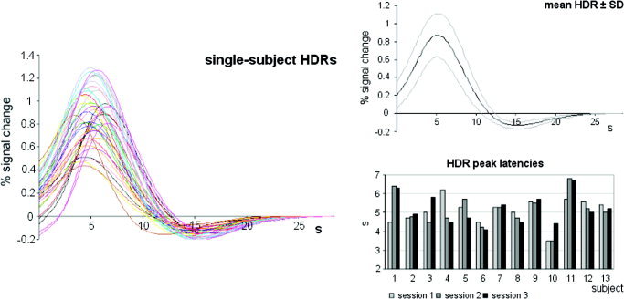
Continuous event‐related image acquisition, fitted data at the global maximum voxel: Left: single subjects' HDRs for each of three sessions are illustrated. Each subject's fitted response curves are kept in one color. The upper graphic on the right shows the HDR averaged across subjects and sessions (black line) ± SD (gray lines), the lower one points out individual latencies of the HDR, again separated for each session (1–3).

HDR maxima of fitted data were 5.11 ± 0.69 s for session 1 (range = 3.5–6.2 s), 5.1 ± 0.88 s for session 2 (range = 3.5–6.8 s), and 5.17 ± 0.78 s for session 3 (range = 4.1–6.7 s; Table I). Peak latencies did not differ significantly between sessions 1–3 (F _1.59 = 0.06, P = 0.904, Greenhouse‐Geisser corrected).

Comparison of Continuous Event‐Related and Sparse fMRI

Calculations of the number of significantly activated voxels in sparse or continuous fMRI revealed large differences between as well as within subjects (Table II). Applying the continuous event‐related technique, the number of statistically relevant activated voxels ranged from 903–17,395 voxels (mean = 8,986.23 ± 4,704.01 voxels). Using sparse acquisition, a minimum of 975 significant voxels and a maximum of 11,999 voxels (mean = 4,320.92 ± 3,161.51 voxels) were found. Continuous event‐related functional imaging revealed significantly more voxels (t = 2.97, P = 0.007) than did sparse fMRI. On average, there was a difference of 4,665.31 ± 5,479.36 voxels between the imaging methods. Under both fMRI designs, 2,845.77 ± 2,367.9 voxels on average were activated significantly. Accordingly, a mean of 36.47± 23.47% voxels activated using continuous event‐related fMRI was also activated during sparse fMRI; 71.17 ± 20.98% of significantly activated voxels during sparse imaging were also included in the continuous imaging activity pattern. At the global maximum voxel, t‐scores ranged from 7.01–18.91 (mean = 12.32 ± 3.27) for continuous event‐related fMRI and from 7.41–25.98 (mean = 13.33 ± 4.71) for sparse imaging. Mean t‐values at the global maximum were not significantly different (t = 0.63, P = 0.532).

Table II.

Single‐subject analyses and mean values

Subject no.	Voxels		Continuous‐sparse	Common	% C in sp	% Sp in c	t
	Continuous	Sparse					Continuous	Sparse
1	4,377	1,075	3,302	853	19.49	79.35	8.41	8.66
2	10,760	4,353	6,407	3,673	34.14	84.38	15.94	12.17
3	9,715	1,997	7,718	1,598	16.45	80.02	13.74	7.41
4	5,806	4,149	1,657	2,824	48.64	68.06	11.49	10.98
5	12,178	1,725	10,453	1,517	12.46	87.94	14.58	8.9
6	8,191	3,907	4,284	2,484	30.33	63.58	12.76	14.77
7	17,395	975	16,420	935	5.38	95.9	18.91	14.99
8	13,355	11,999	1,356	9,100	68.14	75.84	12.18	25.98
9	5,567	5,144	423	2,763	49.63	53.71	12.11	14.59
10	3,908	1,184	2,724	853	21.83	72.04	8.17	12.43
11	903	7,138	−6,235	790	87.49	11.07	7.01	14.95
12	13,860	5,585	8,275	4,280	30.88	76.63	13.67	11.18
13	10,806	6,941	3,865	5,325	49.28	76.72	11.17	16.23
Mean	8,986.23	4,320.92	4,665.31	2,845.77	36.47	71.17	12.32	13.33
SD	4,704.01	3,161.51	5,479.36	2,367.9	23.47	20.98	3.27	4.71

Number of active voxels in continuous event‐related and sparse fMRI, difference in the total number of significant voxels, voxels activated under both imaging schemes, percentage of voxels detected with continuous (c) event‐related fMRI that were also seen using sparse (sp) imaging, percentage of voxels detected applying sparse imaging also found in continuous event‐related fMRI, and t value at the global maximum for continuous and sparse fMRI.

The random‐effects analysis revealed a total of 8,080 voxels with significant t‐values for the conventional event‐related imaging technique with continuous image acquisition. For sparse imaging, this value was 4,100 voxels. The number of significantly activated voxels using either the continuous or sparse imaging scheme was 3,455. The difference in total number of active voxels was 3,980. Of voxels that were identified with the help of continuous image acquisition and appropriate data analysis, 42.76% were also included in sparse imaging activity maps, and 84.27% of sparse imaging voxels with significant t‐values were also activated under conditions of continuous imaging in these analyses. The t‐value at the global maximum was 20.25 in continuous event‐related and 16.81 in sparse fMRI (Table III). Averaged t‐scores of local maxima of both imaging techniques did not differ significantly (t = −0.76, P = 0.45).

Table III.

Multisubject analyses, accounting for random effects

	Voxels		Continuous‐sparse	Common	% C in sp	% Sp in c	t
	Continuous	Sparse					Continuous	Sparse
RFX	8080	4100	3980	3455	42.76	84.27	20.25	16.81

Number of active voxels in continuous event‐related and sparse fMRI, difference in total number of significant voxels, active voxels in continuous event‐related and sparse fMRI, percentage of voxels detected with continuous (c) event‐related that were also seen using sparse (sp) imaging, percentage of voxels detected applying sparse also found in continuous event‐related fMRI, and t value at the global maximum for continuous and sparse fMRI. RFX, random effects.

The random‐effects analysis of both continuously acquired and sparse fMRI data revealed large areas of activation evoked by flashlight stimulation. Activation was observed bilaterally in the occipital lobe within and surrounding the calcarine sulcus. Besides primary cortex, higher visual cortex regions were activated.

Analyzing the continuously acquired event‐related time‐series by random‐effects analysis, a large cluster of activation was found in the occipital lobe with a cluster size of 8,002 voxels (and a comparatively small cluster comprising 78 voxels). Its maximum (global maximum) was located in the right BA 30, surrounded by numerous local maxima situated in BAs involved in visual processing (Table IV). Significant voxels more than 4 mm away from the global maximum were found in BA 17, 18, 19, 23, 28, 30, 31, 35, 37, and 7, including gray matter of the cuneus, lingual gyrus, middle and inferior occipital gyrus, parahippocampal gyrus, posterior cingulate, fusiform gyrus, and precuneus. Activity was also found in the midbrain (colliculi superiores). Figure 3 shows the activation pattern for continuously recorded event‐related functional images revealed by random‐effects analysis.

Table IV.

Typical event‐related design with continuous image acquisition

Gray matter	Hemisphere	BA	x	y	z	t
Cuneus	Left	17	−6	−85	8	13.89
	Right	17	8	−93	6	13.24
Cuneus		18	0	−95	5	15.86
		18	0	−91	8	15.84
	Left	18	−14	−82	28	8.91
		18	−18	−84	24	8.58
		18	−8	−98	14	8.27
		18	−14	−92	18	7.87
	Right	18	10	−83	12	15.46
		18	20	−91	16	10.74
		18	18	−96	18	9.99
		18	20	−82	26	9.04
Lingual gyrus	Left	18	−8	−60	5	11.71
		18	−6	−88	−7	10.31
		18	−10	−68	−3	9.35
		18	−12	−71	−13	9
		18	−10	−76	−11	7.27
	Right	18	4	−78	−13	6.9
Inferior occipital gyrus	Right	18	30	−88	−9	10.29
		18	38	−86	−6	9.74
Middle occipital gyrus	Left	18	−14	−96	14	8.38
Parahippocampal gyrus	Right	19	22	−51	−6	17.1
	Left	19	−20	−55	−2	13.15
Lingual gyrus	Left	19	−12	−47	−6	14.96
Cuneus	Right	19	6	−86	28	12.4
		19	30	−82	28	9.67
		19	16	−94	23	9.53
		19	14	−82	37	9.08
		19	18	−84	34	8.67
	Left	19	−8	−82	34	9.07
		19	−20	−88	28	8.38
		19	−10	−92	27	8.23
		19	−12	−86	30	7.85
Inferior occipital gyrus	Right	19	38	−70	−3	8.01
Cuneus	Left	23	−4	−73	9	18.81
	Right	23	8	−71	11	17.02
Parahippocampal gyrus	Left	28	−18	−27	−5	9.88
Posterior cingulatea	Right	30	16	−66	9	20.25
Parahippocampal gyrus	Left	30	−12	−37	−8	8.21
Posterior cingulate	Right	31	28	−67	18	9.32
Precuneus	Right	31	16	−73	26	9.06
Parahippocampal gyrus	Right	35	20	−35	−5	8.71
Fusiform gyrus	Right	37	38	−57	−11	7.83
		37	40	−61	−9	7.78
Precuneus	Right	7	14	−74	37	9.18
Cuneus	Right	7	14	−74	30	8.92
Colliculi superiores	Right		8	−33	0	9.34
						10.66
Mean (SD)						(3.29)

^aGlobal maximum.

BA, Brodmann area; x, y, z, coordinates in Talairach space.

Figure 3.

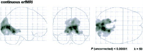
Event‐related design, continuous image acquisition: statistical parametric maps for the random‐effects analysis projected onto the glass brain.

Sparse fMRI data analysis by random‐effects analysis revealed large clusters of activation (cluster sizes = 3,764, 140, 102, and 94 voxels) with a maximum in the right BA 19 (Table V). Local suprathreshold peaks more than 4 mm apart were found in BA 17, 18, 19, 30, 31, 37, and 7. Gray matter of the cuneus, lingual gyrus, fusiform gyrus, parahippocampal gyrus, posterior cingulate gyrus, and precuneus can be assigned to these BAs. Figure 4 illustrates the activation calculated from sparse fMRI data in the multisubject analysis.

Table V.

Local maxima significantly activated during sparse imaging

Gray matter	Hemisphere	BA	x	y	z	t
Cuneus	Right	17	10	−87	10	15.28
		17	4	−89	4	11.9
Cuneus	Left	17	−6	−81	13	10.08
		17	−16	−93	5	7.89
		17	−12	−95	8	7.6
Lingual gyrus	Right	18	14	−72	5	12.45
	Left	18	0	−84	−8	9.46
		18	0	−88	−6	9.41
		18	−10	−84	−9	7.54
Cuneus	Right	18	4	−86	23	10.74
		18	8	−90	17	8.68
		18	16	−86	23	7.94
	Left	18	−2	−73	13	10.54
		18	−10	−97	12	7.6
Fusiform gyrus	Left	18	−18	−86	−14	9.35
Parahippocampal gyrusa	Right	19	22	−56	−2	16.81
		19	20	−51	−4	15.95
Lingual gyrus	Right	19	20	−60	0	13.97
	Left	19	−20	−60	1	12.69
Fusiform gyrus	Right	19	26	−73	−13	11.05
	Left	19	−28	−66	−7	8.22
	Left	19	−34	−65	−10	7.38
Cuneus	Left	19	−20	−90	27	10.19
	Right	19	6	−84	28	8.45
Posterior cingulate	Left	30	−16	−64	9	11.25
		30	−8	−68	9	10.43
Precuneus	Right	31	6	−73	22	8.1
Fusiform gyrus	Left	37	−32	−55	−16	7.47
		37	−38	−63	−10	7.27
		37	−34	−61	−15	6.93
Precuneus	Left	7	−16	−80	35	11.17
						10.12
Mean (SD)						(2.68)

^aGlobal maximum.

BA, Brodmann area; x, y, z, coordinates in Talairach space; SD, standard deviation.

Figure 4.

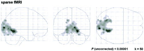
Sparse imaging results: t‐maps of the random‐effects analysis, glass brain views.

Figure 5 illustrates the considerable extent of spatial overlap between t‐maps, acquired by applying the two different image acquisition designs and subsequent data analysis approaches in random‐effects analyses.

Figure 5.

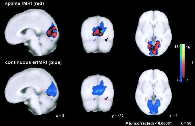
Concordance of activation in both imaging designs: Overlay of t‐maps at Talairach coordinates x = 3, y = −75, z = 4. Top: Sparse fMRI results (red) are superimposed on t‐maps calculated from continuous fMRI data (blue). Bottom: The contrary illustration with sparse imaging results in the background and continuous imaging results in the foreground.

Sensitivity of Sparse Imaging

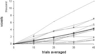
The effect of trial averaging on the sensitivity of sparse fMRI is summarized in Table VI. No signal could be detected if only five trials of stimulation and baseline condition were regarded. On average, 906.15 ± 831.82 suprathreshold voxels were detected including 15 trials, 1,908.77 ± 1,835.67 including 25, 2,987.92 ± 2,489.45 including 35, and 4,320.92 ± 3,161.51 including 45 volumes of each condition into the fMRI model. The repeated measures ANOVA showed a significant effect for the number of trials averaged (F _1.19 = 20.94, P < 0.001, Greenhouse‐Geisser corrected). Each time another 10 images of stimulation and rest were added, the number of activated voxels increased significantly (t = −3.93, P = 0.002; t = −3.26, P = 0.007; t = −4.09; P = 0.001; t = −5.4, P < 0.001; post‐hoc paired comparisons, corrected for multiple comparisons; Table VII). Figure 6 shows the increase of the spatial extent of fMRI activation, depending on the number of trials averaged.

Table VI.

Number of significant voxels and t value depending on number of averaged trials

Parameter	Number of trials
	5	15	25	35	45
Voxels
Mean	0	906.15	1,908.77	2,987.92	4,320.92
SD	0	831.82	1,835.67	2,489.45	3,161.51
Minimum	0	0	0	291	975
Maximum	0	2673	6253	9,199	11,999
t value
Mean	0	9.76	10.24	11.61	13.33
SD	0	4.02	4.29	3.9	4.71
Minimum	0	0	0	6.92	7.41
Maximum	0	15.91	17.43	21.32	25.98

Table VII.

Effect of trial averaging

	Comparison
	5 vs. 15		15 vs. 25		25 vs. 35		35 vs. 45
	t	P	t	P	t	P	t	P
Voxels	−3.93	0.004a	−3.26	0.007a	−4.09	0.004a	−5.4	0.000a
t value	−8.75	0.000a	−1.1	0.3	−2.37	0.071	−3.81	0.007a

Post‐hoc t‐tests (paired comparisons) upon the effect of trial averaging; df = 12 for all comparisons.

^a P < 0.05, corrected for multiple comparisons.

Figure 6.

Number of significant voxels depending on the number of active trials in single‐subjects (thin lines) and averaged across subjects (bold line).

Including 15 trials in the statistical analysis, a mean t‐value of 9.76 ± 4.02 was detected at the global maximum voxel. With increasing number of images, the t‐value of the global maximum increased to a mean t of 10.24 ± 4.29 with 25 trials, 11.61 ± 3.9 with 35, and 13.33 ± 4.71 with 45 trials of visual stimulation and baseline condition analyzed. There was a significant effect for the number of trials averaged as revealed by the repeated measures ANOVA (F _2.17 = 62.91, P < 0.001, Greenhouse–Geisser corrected). Post‐hoc paired comparisons (t‐tests), corrected for multiple comparisons, were statistically significant for the comparison of 5 with 15 trials (t = −8.75, P < 0.001), and 35 with 45 trials (t = −3.81, P = 0.002; Table VII) of each condition. Figure 7 illustrates t‐scores dependent on increasing number of averaged trials.

Figure 7.

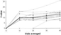
The t‐value at the global maximum depending on the number of active trials in single subjects (thin lines) and averaged across subjects (bold line).

DISCUSSION

The present study used a typical visual paradigm to examine the validity and sensitivity of single‐trial sparse imaging. To our knowledge, neither the validation of the sparse imaging technique via comparison with another established imaging method outside the acoustic domain nor analyses of the effect of trial averaging on sensitivity of this fMRI method have been conducted before. Our results demonstrate that sparse temporal sampling of single brain volumes, combined with a subsequent analysis approach using single‐scan epoch boxcar functions, provides effective detection of activation in the visual cortex.

HDR Peak Latency

Brain volumes in sparse imaging were acquired with a time lag suitable to capture the HDR maximum. This was achieved by calculating the mean HDR and determining its time to peak in our continuously recorded fMRI data. Delayed single volume acquisition in sparse fMRI was then aligned with the computed averaged peak latency. We found the flashlight‐evoked HDR to peak 5.13 ± 0.77 s after stimulus onset for continuously acquired fMRI data, averaged across subjects and sessions 1 to 3. This finding is in line with published fMRI literature about HDR characteristics in visual experiments [Buckner, 1998; Huettel and McCarthy, 2000; Kruggel et al., 2000; Savoy et al., 1995]. The repeated measures ANOVA revealed no significant differences in the mean HDR latency between sessions 1 and 3, confirming our expectation of a stable HDR peak delay for the whole group. This finding was observed averaging only 15 trials of 13 subjects. Nonetheless, as shown in Figure 2, the HDR varied in time to peak across subjects with values ranging from 3.5 to 6.8 s. Consequently, the applied sampling latency was not optimized to capture the HDR peak period in all cases. Small deviations from optimal match of the functional imaging period with subjects' HDR peak period might have affected the statistical power of single‐trial sparse imaging. An individual adaptation of the scanning latency, derived from a preceding similar fMRI experiment with continuous image acquisition instead of an alignment of the scanning latency with the mean value of examined subjects, might further improve the statistical power of the sparse imaging approach.

Comparison of Functional Imaging Approaches

The large variability between subjects' activity patterns using either continuous event‐related or sparse imaging points out discrepancies in individual reactivity. These discrepancies might be explained at least in part by differences in the attentional state between participants. It is known that attention to visual stimuli can modulate the neuronal response to them [Büchel et al., 1998; Spitzer et al., 1988]. In our study, subjects attentively waiting for the next train of flashlights might have shown enhanced activation compared to less alert subjects.

Comparing the two imaging methods regarding single‐subject analyses, the continuous imaging design detected significantly more voxels than did the sparse imaging approach. Under continuous event‐related imaging, approximately twice as many voxels were found. This finding explains why the averaged number of common voxels as well as the percentage of voxels in continuous imaging also detected using sparse temporal sampling is relatively low (36.47%). The contrary perspective revealed a better match: 71.17% of voxels that were found applying sparse fMRI were also seen using continuous event‐related data acquisition. From this point of view, it can be concluded that the sparse imaging approach validly detected the “core activity” revealed using the established event‐related imaging design.

Applying the multisubject random‐effects analyses, the difference in the total number of activated voxels between continuous event‐related and sparse fMRI was comparable to that in averaged single‐subject analyses; however, the concordance between the two imaging schemes was higher. There was an increased amount of overlap between the activation maps, because the random‐effects analysis accounts for subject‐by‐condition interactions [Friston et al., 1999a, b]. The consideration of random effects led to enhanced ratios of voxels found with either method also detected using the other method. Of significant voxels in continuously recorded event‐related imaging data sets, 42.76% were also observed using sparse imaging, and 84.27% of voxels that were captured with the sparse imaging technique were also seen in continuous event‐related imaging. From our results, we conclude that also on multisubject level the spatial extent of significant activity revealed by fitting the HDRs to a basis function (canonical model of the HDR) was larger compared to that attained with the restricted acquisition of a single volume around the HDR peak. Sparse imaging validly detected the main activity that was also seen when using continuous event‐related fMRI. Utilizing random‐effects group analyses, the concordance between the imaging and analysis approaches benefited from reduction of subject‐to‐subject response variability compared to averaged single‐subject statistics.

Beside the spatial extent of the evoked activity and similarities in activation patterns, t‐values were compared on single‐subject (t‐values of global maxima) and multisubject level (t‐values of local maxima). Except for the global maximum voxel reaching a prominent higher t‐value in the random‐effects analysis of continuously acquired images, no differences of statistical relevance in t‐values were found applying either the typical continuous event‐related or the sparse design. Continuous and sparse fMRI results thus differed mainly in the spatial extent detected by these methods but not in their intensity. It therefore has to be taken into account that the two underlying basic approaches to analyze the functional images are different. In case of continuous imaging, 600 images were recorded and each trial onset was convolved with a synthetic HDR function. Moreover, the temporal derivative was added to the design matrix, yielding an optimal fit of empirical data to a theoretical model. In case of sparse imaging, 45 volumes of activation were compared to 45 volumes of rest using a boxcar function. As already mentioned, the sampling delay derived from the continuous data set did not lead to an exact hit of the HDR peak in sparse imaging in all subjects due to variability across subjects in the HDR peak latency. Moreover, it is known that the HDR varies in timing across brain regions [Miezin et al., 2000]. It applies to our results that sparse imaging effectively detects what we labeled the core activity revealed by continuous fMRI and corresponding analysis. Activity around this core region might possess divergent HDR peak latencies. The inclusion of the temporal derivative in conventional event‐related data analysis allows the statistical model to account for timing variability of the BOLD response [Hopfinger et al., 2000]. However, in sparse imaging the scanning latency is fixed and adapted to the HDR peak latency of the core area. Consequently, sparse imaging might have failed to record BOLD signal changes high enough to survive the critical threshold in regions with altered HDR peak latency adjacent to the core area.

Regarding the multisubject analyses, the application of both paradigms led to large clusters of activation in striate and extrastriate visual cortex. Continuous event‐related and sparse fMRI evoked significant changes in BOLD signal not only in BA 17, but also in a variety of higher visual areas. Similar results from blocked design studies were reported by Miki et al. [2000] and Rombouts et al. [1998] with extended activation within and adjacent to the occipital lobe at 8 Hz flashing using a 1.5‐Tesla as well as a 4‐Tesla [Miki et al., 2001] scanner. These findings are not surprising, as it is well known that the primary visual cortex is functionally heterogeneous and has multiple parallel outputs to higher visual areas, which are specialized in processing specific aspects of visual stimuli [Zeki, 1997]. A rather nonspecific stimulus such as a flashlight arouses widespread activity in visual networks.

We observed a displacement of the global maximum when comparing the random‐effects analyses results of continuous event‐related and sparse imaging data. The specific meaning of this finding is difficult to interpret, because the spatial extent of activation maps, at least of the core activity, is largely overlapping. It might be explained by an observation of Miki et al. [2000], who found variable visual activation not only between subjects but also within the same subject. They observed high reproducibility of visual activation using the same paradigm in some subjects but large variations of activated areas in others. The shift of the global maximum activity present in our data might also be ascribed to such intraindividual variance.

Acquisition Time and Sensitivity in Sparse fMRI

A major constraint pertaining to sparse‐related imaging techniques is a prolongation of the total acquisition time caused by: (1) comparatively long interstimulus intervals; and (2) the concomitant need to sample a sufficient number of trials.

The repetition time of imaging epochs must be of sufficient length to ensure the complete recovery of the HDR to the preceding stimulus. Otherwise, activation originating from the previous event cannot be distinguished from the present one, because the provoked HDRs would accumulate. Admittedly, approaches to separate the activation induced by even rapidly presented stimuli [Boynton et al., 1996; Dale and Buckner, 1997; Miezin et al., 2000] assume that the BOLD responses to discrete and rapidly sequenced events summate in a linear fashion and can be deconvoluted to separate the contributions of each stimulus. However, there are indications of nonlinearities [Boynton et al., 1996; Dale and Buckner, 1997; Rosen et al., 1998] and refractory periods [Huettel and McCarthy, 2000] in the HDRs to rapidly presented items. Consequently, there is a persistent uncertainty, if the calculated activation is the same as for stimuli with a longer interstimulus interval [Miezin et al., 2000]. In our study, functional sparse imaging was restricted to a single point in time, not allowing deconvolution methods of continuous time series. We decided in favor of events widely spaced in time to ensure the return of the impulse response curve to baseline level, thus minimizing refractory effects of the HDR [Huettel and McCarthy, 2000]. The expected HDR peak was measured to optimize the statistical power of subsequent data analysis.

Statistical power of sparse imaging data is also lower in comparison to continuous event‐related imaging or a blocked design data because of the smaller number of acquired images at a comparable experimental duration. The signal change with a range of usually 1–3% at a field strength of 1.5 Tesla is relatively small and therefore difficult to detect against background noise [Miki et al., 2001]. To obtain a measurable contrast, an adequate number of trials has to be recorded that can be averaged during subsequent data processing. With simultaneous consideration of an adequate interscan interval, this results in a prolonged acquisition time span. According to a study by Huettel and McCarthy [2001], 25–36 trials are sufficient to estimate the HDR, which was not our goal but served as a clue for the minimal number of trials necessary to obtain a stable measured value. Further improvements could be achieved by adding more trials [Huettel and McCarthy, 2001]. For this reason, we expanded the number of trials to 45 trials, resulting in an experimental duration of approximately 40 min.

Subsequent analyses on the effect of trial averaging upon the number of significantly activated voxels and the magnitude of the t‐score at the global maximum voxel confirmed our decision to include 45 trials of active visual stimulation in comparison to 45 trials of a baseline condition in data analysis. No signal could be detected against background noise if only five trials of each condition were included in the fMRI model. The number of activated voxels and the t‐scores both increased with increasing number of trials analyzed. Significant improvements of the t‐value were observed discontinuously comparing 5 with 15, and 35 with 45 active trials. There were no improvements of statistical relevance in‐between. In contrast, the spatial extent increased whenever additional trials were considered. The latter finding is in line with results reported by Huettel and McCarthy [2001], who investigated the influence of signal averaging on the number of active voxels. They found that when only few trials were averaged, the addition of further trials considerably enlarged the spatial extent. The increase in the number of activated voxels could be described by an exponential function with asymptotic values not approached before averaging 150 trials. The performance of 150 trials of visual stimulation and 150 trials of a baseline condition would last 125 min using our interscan interval in sparse fMRI. The present results suggest that applying a visual paradigm, averaging 15 trials each of an active and a baseline condition are sufficient to detect any activity. In this case, an experimental duration of 12.5 min is achieved. Because the t‐value benefits from averaging more than 35 trials of each condition, and because the spatial extent is measured more accurately the greater the number of averaged trials, we recommend carrying out more than 35 trials of active stimulation, considering that the total acquisition time then exceeds 30 min. The number of trials is limited by the experimental duration, which should, according to participants' statements, not exceed three‐quarters of an hour due to discomfort in the scanner.

To sum up, even if the disadvantage of sparse imaging may be a prolonged experimental duration, the advantage of scanner‐related artifact‐free periods might be substantial for specific experimental demands. The method remains promising, because it validly and effectively detects brain activation, as shown by the presented comparison with more conventional data acquisition and analysis. Future research may prove that single‐event sparse imaging designs, as described in the present study, enable a parallel registration of hemodynamic changes and alterations of further biosignals (e.g., electroencephalography) in response to identical stimuli and in the absence of interfering artifacts resulting from switching magnetic field gradients. Further work is also needed to clarify whether similar stable results can be achieved using sparse temporal sampling for brain regions involved in higher cognitive functions. Müller et al. [2003] already successfully used sparse fMRI to study an auditory oddball task, contrasting images in response to standard nontarget stimuli against those to target stimuli; however, it might apply to experiments on cognitive processing that widespread networks are recruited. If activation is assumed to occur in distinct regions, it has to be taken into account that the HDR peak latency of these regions may differ in the range of seconds [Miezin et al., 2000]. An adaptation of the scanning delay in sparse fMRI to capture the HDR peak as accurately as possible in one region might be disadvantageous in another region with different peak delay. Sparse imaging thus requires previous knowledge about temporal characteristics and position of the BOLD signal changes. If this information is given, sparse imaging can be applied successfully to cognitive experiments.

CONCLUSIONS

The comparison of sparse fMRI with conventional event‐related image acquisition and data analysis shows the validity of the sparse imaging technique within the visual domain. The intensity of signal changes found using either sparse or continuous event‐related fMRI was similar, but conventional fMRI was superior in detecting the spatial extent of activation. The sensitivity of sparse fMRI might be improved by consideration of individual HDR peak latencies, and depends also on the number of averaged trials. Depending on the aim or the available experimental duration of a study, this number can be varied. Few trials are sufficient to detect any activity. A larger number of averaged trials provides more comprehensive measurements. Sparse imaging provides the opportunity to acquire functional imaging data and further biosignals not confounded by scanner‐related artifacts in a broad range of experiments.

REFERENCES

- Backes WH, van Dijk P (2002): Simultaneous sampling of event‐related BOLD responses in auditory cortex and brainstem. Magn Reson Med 47: 90–96. [DOI] [PubMed] [Google Scholar]
- Bandettini PA, Jesmanowicz A, Van Kylen J, Birn RM, Hyde JS (1998): Functional MRI of brain activation induced by scanner acoustic noise. Magn Reson Med 39: 410–416. [DOI] [PubMed] [Google Scholar]
- Belin P, Zatorre RJ, Hoge R, Evans AC, Pike B (1999): Event‐related fMRI of the auditory cortex. Neuroimage 10: 417–429. [DOI] [PubMed] [Google Scholar]
- Birn RM, Bandettini PA, Cox RW, Shaker R (1999): Event‐related fMRI of tasks involving brief motion. Hum Brain Mapp 7: 106–114. [DOI] [PMC free article] [PubMed] [Google Scholar]
- Boynton GM, Engel SA, Glover GH, Heeger DJ (1996): Linear systems analysis of functional magnetic resonance imaging in human V1. J Neurosci 16: 4207–4221. [DOI] [PMC free article] [PubMed] [Google Scholar]
- Büchel C, Josephs O, Rees G, Turner R, Frith CD, Friston KJ (1998): The functional anatomy of attention to visual motion. A functional MRI study. Brain 121: 1281–1294. [DOI] [PubMed] [Google Scholar]
- Buckner RL (1998): Event‐related fMRI and the hemodynamic response. Hum Brain Mapp 6: 373–377. [DOI] [PMC free article] [PubMed] [Google Scholar]
- Dale AM, Buckner RL (1997): Selective averaging of rapidly presented individual trials using fMRI. Hum Brain Mapp 5: 329–340. [DOI] [PubMed] [Google Scholar]
- Eden GF, Joseph JE, Brown HE, Brown CP, Zeffiro TA (1999): Utilizing hemodynamic delay and dispersion to detect fMRI signal change without auditory interference: the behavior interleaved gradients technique. Magn Reson Med 41: 13–20. [DOI] [PubMed] [Google Scholar]
- Elliott MR, Bowtell RW, Morris PG (1999): The effect of scanner sound in visual, motor, and auditory functional MRI. Magn Reson Med 41: 1230–1235. [DOI] [PubMed] [Google Scholar]
- Fransson P, Kruger G, Merboldt KD, Frahm J (1998): Temporal characteristics of oxygenation‐sensitive MRI responses to visual activation in humans. Magn Reson Med 39: 912–919. [DOI] [PubMed] [Google Scholar]
- Friston KJ, Holmes AP, Worsley KJ, Poline JB, Frith CD, Frackowiack RSJ (1995): Statistical parametric maps in functional imaging: A general linear model approach. Hum Brain Mapp 2: 189–210. [Google Scholar]
- Friston KJ, Holmes AP, Price CJ, Büchel C, Worsley KJ (1999a): Multisubject fMRI studies and conjunction analyses. Neuroimage 10: 385–396. [DOI] [PubMed] [Google Scholar]
- Friston KJ, Holmes AP, Worsley KJ (1999b): How many subjects constitute a study? Neuroimage 10: 1–5. [DOI] [PubMed] [Google Scholar]
- Friston KJ, Josephs O, Rees G, Turner R (1998): Nonlinear event‐related responses in fMRI. Magn Reson Med 39: 41–52. [DOI] [PubMed] [Google Scholar]
- Hall DA, Haggard MP, Akeroyd MA, Palmer AR, Summerfield AQ, Elliott MR, Gurney EM, Bowtell RW (1999): “Sparse” temporal sampling in auditory fMRI. Hum Brain Mapp 7: 213–223. [DOI] [PMC free article] [PubMed] [Google Scholar]
- Henson RN, Büchel C, Josephs O, Friston KJ (1999): The slice‐timing problem in event‐related fMRI. Neuroimage 6: 125. [DOI] [PubMed] [Google Scholar]
- Holm S (1979): A simple sequentially rejective multiple test procedure. Scand J Statist 6: 65–70. [Google Scholar]
- Hopfinger JB, Büchel C, Holmes AP, Friston KJ (2000): A study of analysis parameters that influence the sensitivity of event‐related fMRI analyses. Neuroimage 11: 326–33. [DOI] [PubMed] [Google Scholar]
- Huettel SA, McCarthy G (2000): Evidence for a refractory period in the hemodynamic response to visual stimuli as measured by MRI. Neuroimage 11: 547–553. [DOI] [PubMed] [Google Scholar]
- Huettel SA, McCarthy G (2001): The effects of single‐trial averaging upon the spatial extent of fMRI activation. Neuroreport 12: 2411–2416. [DOI] [PubMed] [Google Scholar]
- Janz C, Schmitt C, Speck O, Hennig J (2000): Comparison of the hemodynamic response to different visual stimuli in single‐event and block stimulation fMRI experiments. J Magn Reson Imaging 12: 708–714. [DOI] [PubMed] [Google Scholar]
- Josephs O, Turner R, Friston K (1997): Event‐related fMRI. Hum Brain Mapp 5: 243–248. [DOI] [PubMed] [Google Scholar]
- Kruggel F, Wiggins CJ, Herrmann CS, von Cramon DY (2000): Recording of the event‐related potentials during functional MRI at 3.0 Tesla field strength. Magn Reson Med 44: 277–282. [DOI] [PubMed] [Google Scholar]
- Lancaster JL, Rainey LH, Summerlin JL, Freitas CS, Fox PT, Evans AE, Toga AW, Mazziotta JC (1997): Automated labeling of the human brain: a preliminary report on the development and evaluation of a forward‐transform method. Human Brain Mapp 5: 238–242. [DOI] [PMC free article] [PubMed] [Google Scholar]
- Lancaster JL, Woldorff MG, Parsons LM, Liotti M, Freitas CS, Rainey L, Kochunov PV, Nickerson D, Mikiten SA, Fox PT (2000): Automated Talairach atlas labels for functional brain mapping. Hum Brain Mapp 10: 120–131. [DOI] [PMC free article] [PubMed] [Google Scholar]
- MacSweeney M, Amaro E, Calvert GA, Campbell R, David AS, McGuire P, Williams SC, Woll B, Brammer MJ (2000): Silent speechreading in the absence of scanner noise: an event‐related fMRI study. Neuroreport 11: 1729–1733. [DOI] [PubMed] [Google Scholar]
- Mazard A, Mazoyer B, Etard O, Tzourio‐Mazoyer N, Kosslyn SM, Mellet E (2002): Impact of fMRI acoustic noise on the functional anatomy of visual mental imagery. J Cogn Neurosci 14: 172–186. [DOI] [PubMed] [Google Scholar]
- McFadzean RM, Condon BC, Barr DB (1999): Functional magnetic resonance imaging in the visual system. J Neuroophthalmol 19: 186–200. [PubMed] [Google Scholar]
- Miezin FM, Maccotta L, Ollinger JM, Petersen SE, Buckner RL (2000): Characterizing the hemodynamic response: effects of presentation rate, sampling procedure, and the possibility of ordering brain activity based on relative timing. Neuroimage 11: 735–759. [DOI] [PubMed] [Google Scholar]
- Miki A, Liu GT, Raz J, Englander SA, Bonhomme GR, Aleman DO, Modestino EJ, Liu CS, Haselgrove JC (2001): Visual activation in functional magnetic resonance imaging at very high field (4 Tesla). J Neuroophthalmol 21: 8–11. [DOI] [PubMed] [Google Scholar]
- Miki A, Raz J, van Erp TG, Liu CS, Haselgrove JC, Liu GT (2000): Reproducibility of visual activation in functional MR imaging and effects of postprocessing. AJNR Am J Neuroradiol 21: 910–915. [PMC free article] [PubMed] [Google Scholar]
- Moelker A, Pattynama PM (2003): Acoustic noise concerns in functional magnetic resonance imaging. Hum Brain Mapp 20: 123–141. [DOI] [PMC free article] [PubMed] [Google Scholar]
- Müller BW, Stude P, Nebel K, Wiese H, Ladd ME, Forsting M, Jueptner M (2003): Sparse imaging of the auditory oddball task with functional MRI. Neuroreport 14: 1597–1601. [DOI] [PubMed] [Google Scholar]
- Ogawa S, Lee TM, Kay AR, Tank DW (1990): Brain magnetic resonance imaging with contrast dependent on blood oxygenation. Proc Natl Acad Sci USA 87: 9868–9872. [DOI] [PMC free article] [PubMed] [Google Scholar]
- Rombouts SA, Barkhof F, Hoogenraad FG, Sprenger M, Scheltens P (1998): Within‐subject reproducibility of visual activation patterns with functional magnetic resonance imaging using multislice echo planar imaging. Magn Reson Imaging 16: 105–113. [DOI] [PubMed] [Google Scholar]
- Rosen BR, Buckner RL, Dale AM (1998): Event‐related functional MRI: past, present, and future. Proc Natl Acad Sci USA 95: 773–780. [DOI] [PMC free article] [PubMed] [Google Scholar]
- Savoy RL; Bandettini PA, Weisskoff RM; Kwong KK, Davis TL, Baker JR, et al. (1995): Pushing the temporal resolution of fMRI: studies of very brief visual stimuli, onset variability and asynchrony, and stimulus‐correlated changes in noise. In: Proceedings of the Society of Magnetic Resonance in Medicine Third Annual Meeting, Nice, France. p 450.
- Spitzer H, Desimone R, Moran J (1988): Increased attention enhances both behavioral and neuronal performance. Science 240: 338–340. [DOI] [PubMed] [Google Scholar]
- Talairach J, Tournoux P (1988): Co‐planar stereotaxic atlas of the human brain. Stuttgart: Thieme. [Google Scholar]
- Yang Y, Engelien A, Engelien W, Xu S, Stern E, Silbersweig DA (2000): A silent event‐related functional MRI technique for brain activation studies without interference of scanner acoustic noise. Magn Reson Med 43: 185–190. [DOI] [PubMed] [Google Scholar]
- Zeki S (1997): Dynamism of a PET image: studies of visual function In: Frackowiak RSJ, Friston KJ, Frith CD, Dolan RJ, Mazziotta JC, editors. Human brain function. San Diego: Academic Press; p 163–181. [Google Scholar]