Automated quality assurance routines for fMRI data applied to a multicenter study

Abstract

Standard procedures to achieve quality assessment (QA) of functional magnetic resonance imaging (fMRI) data are of great importance. A standardized and fully automated procedure for QA is presented that allows for classification of data quality and the detection of artifacts by inspecting temporal variations. The application of the procedure on phantom measurements was used to check scanner and stimulation hardware performance. In vivo imaging data were checked efficiently for artifacts within the standard fMRI post‐processing procedure by realignment. Standardized and routinely carried out QA is essential for extensive data amounts as collected in fMRI, especially in multicenter studies. Furthermore, for the comparison of two different groups, it is important to ensure that data quality is approximately equal to avoid possible misinterpretations. This is shown by example, and criteria to quantify differences of data quality between two groups are defined. Hum Brain Mapp 25:237–246, 2005. © 2005 Wiley‐Liss, Inc.

INTRODUCTION

Many factors contribute to the quality of functional magnetic resonance imaging (fMRI) data and influence the significance and reliability of conclusions drawn from these data. Generally, all factors influencing the quality of fMRI results can be classified into four main categories: (1) experimental design; (2) subject cooperation; (3) MRI hardware; and (4) the analysis methods. Published work has focused largely on experimental design [Della‐Maggiore et al.,2002; Friston,2000; Wager and Nichols,2003], result reliability and variability [Casey et al.,1998; Le and Hu,1997; Maitra et al.,2002; McGonigle et al.,2000; Specht et al.,2003], and there is a huge amount of literature on the topic of fMRI data analysis methods. However, it is also important to establish tools and criteria for the quantitative assessment of experimental fMRI data quality. An extensive approach given by Luo and Nichols [2003] requires a high level of user interaction and it is intended to be applied after processing of statistical results. Methods to achieve this goal in an automated manner are useful in MRI applications [Bourel et al.,1999]. For quality assessment of fMRI data, we adopt a generalized approach and focus on subject cooperation and MR hardware issues so that our proposed methods have wide applicability. Stability of fMRI equipment has been considered less frequently [Simmons et al.,1999; Thulborn, 2002], but it nevertheless remains the main prerequisite for successful fMRI. We present a method, using phantom measurements, for the routine evaluation of echo‐planar imaging (EPI) stability in terms of the percentage signal change (PSC) and statistical noise properties. Controlling subject cooperation is only treated in terms of data quality, which is quite often reduced by motion‐induced artifacts; a generally applicable approach to check subject cooperation is a much more complex task and is very much design related. Paradigms where subjects respond to stimulus events are well suited for evaluation of subject cooperation through the use of behavioral performance data. Subject cooperation in paradigms employing visual stimuli can be examined using MR‐compatible eye‐tracking devices. Moreover, the influence of the mental and physiological state of the subject on the fMRI signal can be checked indirectly in real‐time by tracking additional physiological data [Voyvodic,1999]. Image‐based physiological artifact detection and correction during post‐processing can also be carried out [Chuang and Chen,2001]. However, the decision to follow one or more of these strategies depends strongly on paradigm design and the conclusions expected to be drawn from the experiment. The quality assessment (QA) procedures discussed herein are rooted in basic considerations of, and applicability to, every fMRI design. For each experiment it is necessary to ensure proper scanner performance and EPI image data free of motion‐induced artifacts; these are minimal requirements for further successful post‐processing. Although many different implementations to test compliance with the above requirements can be devised, we present procedures that are easy to implement and require minimal additional work, making them especially suitable for routine application. All quality assessment parameters defined here are given in terms of the PSC, which we believe to be a most instructive measure because in some cases it even allows direct interpretation of whether a temporal signal change is blood oxygenation level‐dependent (BOLD) induced. A temporally localized PSC that exceeds 5%, for example, can hardly be explained by the BOLD effect [Thulborn, 2002]. However, we do not give any significance levels for these parameters because defining such boundaries in a meaningful way to test a hypothesis H₀, such as “H₀ = data quality is not sufficient,” depends strongly on the conceptual framework of a specific experimental design; therefore it needs to be adapted individually. In the framework of a German multicenter study on schizophrenia patients [Schneider et al., submitted] from which this work was developed, we focused our attention on the comparison of fMRI data quality across groups of subjects, and the influence on group comparisons. We present a general concept to avoid misleading interpretations that can arise because of different data quality in the groups. In the Concepts section of this paper, quality assessment measures are derived from theory and clarified further through the use of examples. The Methods section gives a short description of the experimental conditions. We present two representative examples in the Results section, one showing the long‐term assessment of fMRI hardware stability using phantom data and the other showing the strong influence of in vivo data quality on the statistical maps. Data quality can cause serious misinterpretations and a method to prevent this is also described.

Concepts

We present a fully automatic routine for the quality assessment of fMRI data that is retrospectively applicable to every fMRI experiment. It requires only the realigned magnitude images, ensuring that product EPI sequences from different vendors can be used. The accuracy of the motion correction algorithm influences the results of the presented approach; however, the principles remain the same. We thus decided to apply the commonly used realignment procedure as implemented in Statistical Parametric Mapping (SPM2).1 The method yields temporal and slice‐dependent control of artifact‐induced percent signal changes. More importantly, the data quality of one fMRI experimental run is described by only two parameters, one giving the noise level and the other describing the statistical properties of the noise. To achieve these goals, the routine sequentially carried out the steps described below.

Noise‐level detection and image masking

Under ideal conditions, the real and imaginary part of the MR signal have a Gaussian distribution with the same mean and standard deviation, say A and σ. The signal, S, of the magnitude image then has a Rician distribution

(1)

which turns into a Gaussian distribution if A/σ → ∞ and into a Rayleigh distribution if A/σ → 0 [Sijbers et al.,1998]. For SPM2 analysis, it is assumed that A >> σ and the noise distribution can be treated as Gaussian. To restrict QA to the voxels of interest, a mask

(2)

is applied to the registered MR images, where T is a suitable threshold. For example, T = 20 ensures that the Rician and Gaussian distribution are treated equally for the applications presented here. Finding all voxels for which equation (2) holds requires an estimate of the noise level, which is often carried out by inspecting a region‐of‐interest (ROI) of the MR image where no signal is present (background noise method) [Magnusson and Olsson,2000]. The average signal in such a background region, R, is related to the standard deviation by

(3)

Finding a suitable background ROI generally requires user interaction. For an EPI time series, automated detection is possible if σ is assumed to be stationary. We searched in the corners (1/8 of the EPI volume) of the first scan for some minimal values to ensure that background data were obtained. These voxels were tracked through the whole time series and σ was computed according to equation (3). The method yielded the same results as those achieved through user interaction, i.e., manual definition of a background ROI in one scan. For in vivo measurements, the mask usually contained the eyes of the subject, which are generally a source of strong signal variations in the EPI time series. For the QA procedure, it is thus useful to apply eye masking because these variations should not enter the QA calculation. Automated eye masking at the stage of the realigned images can be applied if the mask given by the threshold T yields disconnected regions for the brain and the eyes. For T = 20, this was the case in 100% of our investigated experimental runs.2 Generally, a routine to find a connected region within a 3‐D dataset is time consuming but the EPI datasets are usually small. For our datasets (64 × 64 × 32), a rather simple three‐step routine worked very well. Firstly, edge detection was applied to the mask R _T obtained from the threshold condition [Petrou and Bosdogianni,1999]. Secondly, neighbor detection was carried out to find a region, R _H, yielding all voxels of the hull excluding the eyes. Finally the mask region, R _M, was found by a form of spatial integration of the hull intersected with the threshold mask (see appendix). The method is computationally fast, less than 30 s on a standard PC (2.4 GHz Pentium IV), and it successfully removed the eyes in masks of inspected in vivo fMRI datasets. An example is depicted in Figure 1. Removing the eyes is of course not only beneficial for the QA procedure but also for standard fMRI analysis [Tregellas et al.,2002].

Figure 1.

Fast routine for automated eye removal. From the threshold mask R _T (A), its hull (B) is found by edge detection. The voxels on the hull (C), excluding the eyes, are found by neighbor search. The final mask R _M (D) is determined by intersecting the original mask R _T with the spatial integration R _H of the hull. (See Appendix for details.)

Signal‐distribution properties

In this step we calculate the noise distribution properties and the level of random noise of an experimental fMRI run. First, we expect the noise to be uncorrelated in space and time, which is certainly not true, as reported many times in the literature [e.g., Luo and Nichols,2003]. Our analysis shows the extent to which this assumption is fulfilled and thus it is well suited before any fMRI analysis based on these assumptions. Prewhitening of the data, as applied within the statistical analysis procedure, can also be applied before QA. This is especially useful in short repetition time (TR) experiments. Let S denote the mean image of the EPI time series, i.e., the time‐averaged image. The time series {S(t) − S} is then expected to have zero mean and Gaussian‐distributed noise in every voxel of the mask region. Treating each value as an independent realization of the same probability distribution gives N _t · N _M values, where N _t and N _M are the number of time points and the number of voxels in the mask, respectively. This large number allows an accurate estimation of the distribution‐type. Well‐known methods to test for the type of distribution rely on some form of distance measure, estimating the noise distribution of the data and calculating the difference to some given distribution. A prominent approach is the Kolmogorov–Smirnov distance, which is given by the maximum difference between the cumulative distribution functions (CDF)

(4)

where z is the z‐score, P̃ denotes an estimate of the CDF of the data, and P _SN is the standard normal CDF. This method is insensitive to differences in the tails of the distributions; an improvement is given by the Anderson–Darling distance, which weights the difference by (P _SN[1 − P _SN])^−1/2 [Press et al.,1992]. Both methods are implemented in our automated QA routine. In our opinion, the method of choice is a presentation of the quantiles of the data in comparison to the quantiles of the Gaussian distribution. Here, the inverse function of the CDF, the so‐called “quantile function” of the data, is plotted against the standard normal quantile function. This so‐called q–q plot [Gnanadesikan,1997] shows a linear relationship if the underlying distributions are the same. Mathematically, the q–q plot is given by the mapping

(5)

where Q̃ and Q _SN are P̃⁻¹ and P _SN ⁻¹, respectively (Q̃ is nothing but the sorted data). Because Q _SN maps to z‐scores, deviation in the tails of the distributions can be interpreted easily in numbers of standard deviations. The correlation coefficient

(6)

serves as a single quantity describing the difference of the distribution of the data to the normal distribution. Here, 〈.,.〉 and ∥.∥ are the Euclidian scalar product and norm, respectively. Furthermore, the mean and standard deviation of the distribution can be estimated from the offset and the slope of the q–q plot, respectively. Zero mean is forced because the mean corrected data enter the calculation. The standard deviation σ is an estimate of the level of random noise. We define the percentage signal change (PSC) via the relative error, i.e.,

(7)

The denominator is the mean signal intensity within the mask. If the variance differs strongly from the background noise estimate of variance, then this is generally accompanied by a low correlation coefficient r _qq. This means the noise is not purely random but has coherent components arising most probably from subject‐induced signal changes such as motion artifacts, physiological noise, and BOLD signal changes as well. Figure 2 shows an example of the q–q plot.

Figure 2.

Presentation of the distribution‐type of fMRI data by means of the q–q plot. Data are consistent with the assumption of Gaussian‐distributed data; r _qq and σ are the correlation coefficient and the slope of the data, respectively. They define the similarity to the Gaussian distribution and its standard deviation.

Temporal and spatial variations

To obtain the temporal variation of the QA parameters, the q–q analysis was confined to the data coming from a single scan, i.e., we carried out the calculation on N _M data points N _t times. Equations (6) and (7) thus yield the time‐varying correlation coefficient r _qq(t) and the percent signal change p _σ(t), respectively. The latter quantity is well suited to detect single corrupted scans. A further constraint is to analyze only the voxels within a single slice, allowing the detection of corrupted slices within a corrupted scan. An example of the PSC for an experimental run corrupted by spike artifacts is depicted in Figure 3. Such a representation allows the detection of the corrupted scans and slices.

Figure 3.

Example of the percent signal change (PSC) of an fMRI experimental run corrupted by spikes. SPM2 translational realignment parameters (A) in comparison to the PSC (B). Spikes, which are visible in (B), do not necessarily occur in (A) and vice versa. Only the PSC gives valuable information about the corrupted scans (C) PSC per slice. The marked slice is shown in (D), whereas (E) shows the same slice at the foregoing time‐point and (F) shows the difference.

MATERIALS AND METHODS

A homogenous MR phantom with relaxation times approximating brain tissue was used for routine measurements that replicated an in vivo fMRI experiment. The measurement was carried out once a week on a 1.5‐T Siemens Sonata scanner. The standard Siemens product EPI sequence was used with the following parameters: TR = 5 s; echo time (TE) = 60 ms; flip angle 90 degrees; 32 slices; slice thickness 3 mm; filed of view (FOV) = 200 mm (rectangular); matrix size 64 × 64; 96 measurements. First, we discarded three measurements to reach steady state (prescans). TR denotes the acquisition time of one measurement (volume scan); the acquisition time for one slice was approximately 100 ms and therefore a dead‐time of approximately 1.8 s was included in TR. Motion correction was applied to the phantom data because gradient heating results in biased position encoding in long EPI acquisitions (Fig. 4). QA analysis was carried out after the phantom measurements, as described in the previous section, to enable consideration of the QA parameters. In vivo experiments were also processed in the same way with the additional step of automated eye removal, which was applied as a first step of QA to ensure that the QA parameters were not influenced by signal intensity variations caused by eye movement. As for the phantom measurements, it is of great advantage to have a single quantity describing the data quality of an in vivo experiment. The correlation coefficient r _qq is well suited, as explained in more detail below. However, a temporally integrated measure for the in vivo data quality should not include BOLD‐induced signal variations. Those variations will violate the assumption of a stationary probability distribution and, consequently, the BOLD signal will decrease r _qq. We therefore ran the QA twice. First, all time points are included to detect possible corrupted single scans and slices. In the second run, we incorporated only those scans into the QA analysis that fall within the baseline condition of the fMRI experiment. This allows determination of the QA quantities r _qq and p _σ unaffected by BOLD signal variations. For the multicenter study, this is depicted in Figure 5. BOLD variations of interest should thus no longer decrease r _qq. If this strategy is not applicable, e.g., in an event‐related design, it might be necessary to mask regions where high BOLD signal variations are expected to occur.

Figure 4.

Scanner drift in an EPI time course of a phantom measurement is illustrated by the realignment parameters (A). The q–q analyses of the raw data (B) and the realigned data (C) differ significantly in their tails. Gradient heating in the readout direction causes small shifts in the spatial encoding. Without correction, the MR signal distribution has the appearance of being non‐Gaussian; this is a consequence of ignoring the shift.

Figure 5.

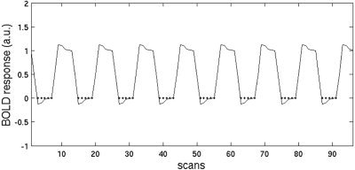
QA of in vivo data. The hemodynamic model of the baseline condition defines the data that are taken into account. Dots mark the scans used for the q–q analysis for each subject so that BOLD‐induced signal variations do not influence the QA.

RESULTS

Long‐Term Assessment of fMRI Hardware Stability

We present data from the above‐mentioned multicenter study that were acquired at seven different institutes all using 1.5 T Siemens MR scanners. The amount of contributed data was distributed rather heterogeneously among the centers, e.g., 35% of the in vivo data and 54% of the phantom data were acquired at our institute. The long‐term QA of phantom measurements within the multicenter study is depicted in Figure 6. It shows the PSC for the seven contributing centers acquired during the past 3 years. Two centers (shown by diamonds and asterisks) had significantly long periods with a higher PSC. To establish whether the high noise level was purely random or if artifacts were present, the statistical properties of the noise were investigated. Figure 7 depicts the results for the three different kinds of distribution‐type similarity measures: the Kolmogorov–Smirnov distance, D _KS; the q–q plot correlation coefficient, r _qq, and the Anderson–Darling distance, D _AD. D _KS and r _qq are highly correlated, because both measures are sensitive to changes near the mean of the distribution, whereas D _AD is more sensitive to changes in the tails. Spike artifacts, which spread out all over the volume of some selected scans and slices, are detected better with D _KS or r _qq. Artifacts that occur only in a very limited number of voxels but with strong signal change are better detected with D _AD. The latter kind of artifacts was present at the center depicted by diamonds in the graph because of serious hardware problems (which have since been solved by the vendor). Spike artifacts were found at the center depicted by plus signs for a period in late 2001 and again in spring 2003. All these variations in hardware stability are summarized well by the QA analysis. To ensure data acquisition of a consistently high quality, the proposed parameters to quantify the magnitude of the noise and its statistical properties, respectively, must be calculated directly after each measurement so that problems may be detected as early as possible and remedial action may be taken as necessary. This consequence might, intuitively, be a matter of course. The multiplicity of hardware problems detected by the long‐term QA clearly underlines the need for QA in fMRI.

Figure 6.

Percent signal change (PSC) of all phantom measurements in the multicenter study. The symbols denote the seven contributing centers. A high PSC denotes a high noise level. The PSC, however, cannot distinguish between random noise and coherent noise (artifacts). For this, the distribution type has to be considered (Fig. 7).

Figure 7.

Distribution‐type estimate for all phantom measurements in the multicenter study. The difference from a Gaussian distribution is shown in (A), (B), and (C) by the Kolmogorov–Smirnov distance D _KS, the q–q correlation coefficient r _qq, and the Anderson–Darling distance D _AD, respectively. Generally, a zero KS or AD distance, as well as a q–q correlation coefficient of one, denote that the noise in the underlying data is purely random (normally distributed) and no MR artifacts are present. Table (D) shows how these measures correlate with each other. Although (A) and (B) are sensitive to variations in the mean of the distribution, (C) is more sensitive to changes in the tails.

Quality Assessment of In Vivo Data

The inspection of automatically generated processing results, most importantly from the PSC time series, gives valuable information about corrupted scans and slices (Fig. 3). This information might be used for corrections such as interpolation to remove the corrupted scans/slices. The overall data quality is described by the single quantity r _qq, which is calculated based on baseline scans of the fMRI experiment. As r _qq is sensitive to changes near the mean of the estimated probability distribution of the data, it is related closely to Student's t‐test, the method of choice in fMRI data analysis (SPM2). The t‐test is based on differences of mean values between different conditions, both of which follow a Gaussian distribution. Optimal data quality, given by r _qq = 1, thus reflects the prerequisites of the t‐test. The r _qq was calculated for each in vivo data set of the multicenter study, which involved 71 patients and 71 control subjects. Here, the question of whether the data quality is different between the two groups arises, and if so, what the consequences are for inferences from fMRI data analysis. To address these questions, Figure 8a shows a rank‐ordered plot of the r _qq for control subjects versus that for patients. This representation is itself a q–q plot, where the underlying distribution of r _qq is not known. If it shows the same distribution for both groups, then the q–q plot is a straight line that crosses the origin and has slope of unity. This q–q plot is therefore a distribution‐free quantification of the differences in the statistical properties of the data from both groups. The same argument holds for the amount of random noise given by the PSC, as shown in Figure 8b. Together, the assumption of equal data quality in both groups is well met in the case of the multicenter study. Defining thresholds for the parameters that describe acceptable similarity of the distributions is a difficult question that requires investigation in future work. We show only by example that a strong violation of the assumption of equal data quality in both groups strongly influences the results of the fMRI data analysis. We take the upper and lower tail of both groups, defining subgroups with high and low data quality, respectively. For this, the noise level as described by the PSC is a more natural choice than are the statistical properties given by r _qq. The subgroups were defined by the 16 subjects with the lowest and highest PSCs, respectively. Due to the tight matching criteria of the study, the subgroups remained matched among each other in terms of age, gender, and educational level. Patient and control groups are denoted with P and C, and high/low data quality is given by the superscripts +/−, respectively. These groups were used for standard fMRI random‐effects analysis with SPM2. We carried out one‐sample t‐tests on these groups as well as two‐sample t‐tests for the comparisons P⁺–C⁻, P⁻–C⁺, C⁺–P⁻, and C⁻–P⁺. These results are discussed in terms of data quality and the level of activation. A detailed description of this study and interpretation of the results can be found in Schneider et al. [submitted]. It is sufficient to note here that the fMRI task was a 0‐back/2‐back continuous performance test, where the 0‐back task is an attention condition, and the 2‐back task is an attention and short‐term working memory condition. Single‐subject analysis was carried out for the difference of these two conditions, thus showing basically the activation related to working memory. One‐sample t‐test results of the subgroups are shown in Figure 9. The amount of activation clearly correlates with the data quality, as expected. A similar observation holds for the two‐sample t‐tests shown in Figure 10. Strong activations are present if the group to be subtracted has low data quality, and vice versa. The results of the comparison P–C and C–P thus depend strongly on the data quality of the groups. If the data quality of the groups is not approximately equal, the resulting activations can lead to a serious misinterpretation of the results. To prevent this, a group comparison of data quality is necessary, as shown here.

Figure 8.

QA of fMRI data in patient studies. The q–q correlation coefficients r _qq of the patient data are plotted vs. r _qq of the control data, yielding another q–q plot (A). Its correlation coefficient r describes the consistency of the distribution type of r _qq for both groups. The parameters of a linear fit (μ and σ²) describe their deviation in mean and variance; thus, ideally, r = 1, μ = 0, and σ = 1 holds for the comparison of fMRI data quality of two groups. The same procedure is also applied to the PSC of all subjects (B). Because the PSC reflects the amount of random noise, the trend shows that subjects with lower PSC show higher activations in fMRI data analyses. For the data presented here, the influence of data quality on group comparisons is negligible because the amount of random noise (PSC) and statistical properties of the noise (r _qq) follow very similar distributions across both groups.

Figure 9.

SPM2 one‐sample t‐test results (random effects) for the working memory contrast in the multicenter study. Groups of size n = 16 were analyzed; C, controls subjects; P, patients; +/−, lowest/highest PSC (highest/lowest data quality), respectively. All results are thresholded at P < 0.001 (uncorrected). C⁺ and C⁻ results are similar; however, C⁺ strongest activation corresponds to a t‐value of 14, whereas C⁻ does not contain t‐scores above 9.5. Furthermore, the cluster size is larger in the C⁺ group. The P⁻ group has extremely low data quality, which is reflected by the low activation in the statistical maps. It is the only case that does not show any activation when thresholding at P < 0.05 with correction for multiple comparisons.

Figure 10.

SPM2 two‐sample t‐tests (random effects) comparing the results of the groups depicted in Figure 9. Groups with low data quality (C⁻,P⁻) do not show more activations than do groups with high data quality (C⁺,P⁺). The contrasts (C⁺–P⁻) and (P⁺–C⁻) show significant activations at the chosen threshold, P < 0.001 (uncorrected); this activation can also partly be seen when thresholding at P < 0.05 with correction for multiple comparisons. The results clearly show that the activation patterns in group comparisons are influenced strongly by the data quality of each group. For instance, the contrasts (C⁺–P⁺) and (P⁺–C⁺) (not shown here) resemble the first and the third activation patterns shown above, but with lower activations. The strength of activations in group comparisons thus can only be interpreted if data quality is equal across both groups.

DISCUSSION

The possible sources of corrupted data collected in fMRI are manifold. The data can be corrupted by randomly distributed noise, coherent noise (artifacts), or both. On the one hand, this can be caused directly by the MR scanner, especially when using EPI, which is used widely in fMRI because it provides high temporal resolution but it is extremely demanding on the imaging hardware. On the other hand, fMRI stimulation devices (e.g., visual/audio, response devices) and also monitoring devices (e.g., eye tracking, physiologic monitoring, electroencephalography [EEG]) brought into the scanner room are all possible sources for both types of noise. For these reasons, quality assessment of the hardware has to be carried out under exactly the same conditions as for the in vivo experiments. Testing the quality of EPI, for example, in the absence of the whole stimulation/monitoring environment potentially disregards important sources of error. The procedure of phantom data acquisition and automatic processing presented here yields several QA parameters. For our purposes, we found that the overall PSC should not exceed 1.5%. Testing the data for statistical properties is carried out by inspecting the q–q correlation coefficient r _qq and data with r _qq > 0.9 seem to be very acceptable. These numbers were found on an empirical basis at our site; all measurements that violated these thresholds could be assigned clearly to problems in the hardware set‐up on that specific day. If a single phantom measurement exceeds these limits, tests on the fMRI hardware environment have to be carried out immediately. These thresholds might be different in different situations such as various experimental designs or static field strengths. The concepts described here may be applied directly in such situations. For QA of in vivo data, the time series of the PSC allows detection of corrupted scans and slices, which might be amenable to interpolation in post‐processing. Again, the PSC and r _qq are good measures for the consistency of fMRI data in a group study. Neglecting data sets with high PSC (low r _qq) might strengthen the inference of results; however, it is important that the parameters do not vary strongly across two different groups in a group comparison or patient study. This is a dangerous source of possible misinterpretations of the results. To ensure that data quality is approximately equal for both groups, we carried out a second q–q analysis on the PSC and r _qq of all subjects from patient and control groups. This allowed quantification of the deviation in data quality for different groups of subjects. It is shown by example that strong deviations in the fMRI analysis results (achieved with SPM2) can be obtained by investigating groups with strongly different data quality. Methods to quantify the differences in data quality are given so that misinterpretations of group comparisons can be avoided.

CONCLUSIONS

We present efficient, standardized, easy‐to‐implement, and easy‐to‐automate procedures for quality assessment of fMRI data. Such methods should be applied on a routine basis in every fMRI study because the possible sources of data corruption in fMRI are manifold. We divided these sources into three main categories: (1) experimental design; (2) subject cooperation; and (3) fMRI hardware. We focused on assessment of hardware‐induced artifacts and subject‐induced data corruption during the experimental runs. The goal to define sensitive parameters acting as “warning flags” in an automated manner was achieved. These newly defined QA parameters integrate over all possible sources of unwanted signal variance. However, combination with other approaches, such as detection of only physiologically induced noise, remains to be addressed. This may be applicable only if the specific design and the underlying neuroscientific hypotheses are also taken into account. Many approaches that address these issues have been published; however, a standardized (and if possible, automated) implementation is of great practical importance for day‐to‐day application in fMRI. Because BOLD signal detection remains crucial, the inference of fMRI results can only reach a clinical standard if QA is considered exhaustively.

The automated eye removal, briefly discussed in the Concepts section, is fast because the time‐consuming neighbor detection has to be carried out only on the limited number of voxels on the hull R _H, found by the edge detection. Finding the interior of any 3D hull is generally also a nontrivial and time‐consuming task, so the problem only seems to have been shifted. For the special case of eye removal of EPI volumes, however, there is very fast way to achieve this aim. Let R _H ^i,j,k denote the region describing the hull, which equals either 1 if {i,j,k} denotes a voxel on the hull, or 0 elsewhere. We then can quickly compute six regions defined by the cumulative sums starting from each side of the N _x × N _y × N _z cube:

(8)

(9)

(10)

(11)

(12)

(13)

where sign[ · ] denotes the signum function. It is easy to see that the target mask region R _M, i.e., the head excluding the eyes, is a subset of each of these sums, and it is thus also a subset of its intersection. This intersection is generally larger, but it always excludes the eyes. R _M is therefore found efficiently by a further intersection with the original thresholded mask R _T:

(14)

REFERENCES

- Bourel P, Gibon D, Coste E, Daanen V, Rousseau J (1999): Automatic quality assessment protocol for MRI equipment. Med Phys 26: 2693–2700. [DOI] [PubMed] [Google Scholar]
- Casey BJ, Cohen JD, O'Craven K, Davidson RJ, Irwin W, Nelson CA, Noll DC, Hu X, Lowe MJ, Rosen BR, Truwitt, CL , Turski PA (1998): Reproducibility of fMRI results across four institutions using a spatial working memory task. Neuroimage 8: 249–261. [DOI] [PubMed] [Google Scholar]
- Chuang KH, Chen JH (2001): IMPACT: Image‐based physiological artifacts estimation and correction technique for functional MRI. Magn Reson Med 46: 344–353. [DOI] [PubMed] [Google Scholar]
- Della‐Maggiore V, Chau W, Peres‐Neto PR, McIntosh AR (2002): An empirical comparison of SPM preprocessing parameters to the analysis of fMRI data. Neuroimage 17: 19–28. [DOI] [PubMed] [Google Scholar]
- Friston KJ (2000): Experimental design and statistical issues In: Mazziotta JC, Toga AW, Frackowiak RSJ, editors. Brain Mapping: the disorders. San Diego: Academic Press; p 33–58. [Google Scholar]
- Gnanadesikan R (1997): Methods for statistical data analysis of multivariate observations. Second ed. New York: John Wiley & Sons; 384 p. [Google Scholar]
- Le TH, Hu X (1997): Methods for assessing accuracy and reliability in functional MRI. NMR Biomed 10: 160–164. [DOI] [PubMed] [Google Scholar]
- Luo WL, Nichols TE (2003): Diagnosis and exploration of massively univariate neuroimaging models. Neuroimage 19: 1014–1032. [DOI] [PubMed] [Google Scholar]
- Magnusson P, Olsson LE (2000): Image analysis methods for assessing levels of image plane nonuniformity and stochastic noise in a magnetic resonance image of a homogenous phantom. Med Phys 27: 1980–1994. [DOI] [PubMed] [Google Scholar]
- Maitra R, Roys SR, Gullapalli RP (2002): Test–retest reliability estimation of functional MRI Data. Magn Reson Med 48: 62–70. [DOI] [PubMed] [Google Scholar]
- McGonigle DJ, Howseman AM, Athwal BS, Friston KJ, Frackowiak RSJ, Holmes AP (2000): Variability in fMRI: an examination of intersession differences. Neuroimage 11: 708–734. [DOI] [PubMed] [Google Scholar]
- Petrou M, Bosdogianni P (1999): Image processing: the fundamentals. New York: John Wiley & Sons; 354 p. [Google Scholar]
- Press WH, Tukolsky SA, Vetterling WT, Flannery BP (1992): Numerical recipes in C: the art of scientific computing. New York: Cambridge University Press. 1020 p. [Google Scholar]
- Schneider F, Habel U, Klein M, Kellermann T, Stöcker T, Shah NJ, Zilles K, Braus DF, Schmitt A, Schlösser R, Friederich M, Wagner M, Frommann I, Kircher T, Rapp A, Meisenzahl E, Ufer S, Ruhrmann S, Thienel R, Sauer H, Henn FA, Gaebel W (Submitted): A multi‐center fMRI study of cognitive dysfunction in first‐episode schizophrenia patients. Am J Psychiatry. [DOI] [PubMed]
- Sijbers J, den Dekker AJ, Van Audekerke J, Verhoye M, Van Dyck D (1998): Estimation of the noise in magnitude MR images. Magn Reson Imaging 16: 87–90. [DOI] [PubMed] [Google Scholar]
- Simmons A, Moore E, Williams SC (1999): Quality control for functional magnetic resonance imaging using automated data analysis and Shewhart charting. Magn Reson Med 41: 1274–1278. [DOI] [PubMed] [Google Scholar]
- Specht K, Willmes K, Shah NJ, Jäncke L (2003): Assessment of reliability in functional imaging studies. J Magn Reson Imaging 17: 463–471. [DOI] [PubMed] [Google Scholar]
- Thulborn KR (2000): Quality assurance in clinical and research echo planar functional MRI In: Moonen CTW, Bandettini PA, editors. Functional MRI. Berlin: Springer‐Verlag; p 337–346. [Google Scholar]
- Tregellas JR, Tanabe JL, Miller DE, Freedman R (2002): Monitoring eye movements during fMRI tasks with echo planar images. Hum Brain Mapp 17: 237–243. [DOI] [PMC free article] [PubMed] [Google Scholar]
- Voyvodic JT (1999): Real‐time fMRI paradigm control, physiology, and behavior combined with near real‐time statistical analysis. Neuroimage 10: 91–106. [DOI] [PubMed] [Google Scholar]
- Wager TD, Nichols TE (2003): Optimization of experimental design in fMRI: a general framework using a genetic algorithm. Neuroimage 18: 293–409. [DOI] [PubMed] [Google Scholar]