Source density‐driven independent component analysis approach for fMRI data

Abstract

Independent component analysis (ICA) has become a popular tool for functional magnetic resonance imaging (fMRI) data analysis. Conventional ICA algorithms including Infomax and FAST‐ICA algorithms employ the underlying assumption that data can be decomposed into statistically independent sources and implicitly model the probability density functions of the underlying sources as highly kurtotic or symmetric. When source data violate these assumptions (e.g., are asymmetric), however, conventional ICA methods might not work well. As a result, modeling of the underlying sources becomes an important issue for ICA applications. We propose a source density‐driven ICA (SD‐ICA) method. The SD‐ICA algorithm involves a two‐step procedure. It uses a conventional ICA algorithm to obtain initial independent source estimates for the first‐step and then, using a kernel estimator technique, the source density is calculated. A refitted nonlinear function is used for each source at the second step. We show that the proposed SD‐ICA algorithm provides flexible source adaptivity and improves ICA performance. On SD‐ICA application to fMRI signals, the physiologic meaningful components (e.g., activated regions) of fMRI signals are governed typically by a small percentage of the whole‐brain map on a task‐related activation. Extra prior information (using a skewed‐weighted distribution transformation) is thus additionally applied to the algorithm for the regions of interest of data (e.g., visual activated regions) to emphasize the importance of the tail part of the distribution. Our experimental results show that the source density‐driven ICA method can improve performance further by incorporating some a priori information into ICA analysis of fMRI signals. Hum Brain Mapping, 2005. © 2005 Wiley‐Liss, Inc.

INTRODUCTION

Independent component analysis (ICA) is becoming a popular tool for biomedical signal analysis. Since Infomax‐based ICA was introduced for biomedical data processing [Bell and Sejnowski, 1995], a number of ICA approaches are emerging for functional magnetic resonance imaging (fMRI) signal analysis [Biswal and Ulmer, 1999; Calhoun et al., 2001a; Dodel et al., 2000; McKeown et al., 1998; Stone et al., 2002; Suzuki et al., 2001]. Among these successful applications, the primary assumption is that there are statistically independent mixed sources, and current algorithms typically model (either implicitly or explicitly) the probability density functions (pdf) of the underlying sources as symmetric or highly kurtotic. This assumption might be inconsistent with the situation for fMRI data; fMRI data can be considered to contain many underlying sources, but not all would be expected to be symmetric [Calhoun et al., 2001a]. For example, the task‐related underlying source is skewed if it consists of only activated or deactivated voxels [Suzuki et al., 2001]. There have been some attempts to examine the underlying assumptions of ICA [Calhoun et al., 2001c; McKeown and Sejnowski, 1998; McKeown, 2000; Porrill et al., 2000] and to modify the underlying probability models (i.e., assumptions) to be more suitable for fMRI signal analysis [Nakada et al., 2000; Stone et al., 2002; Suzuki et al., 2001]. Biswal and Ulmer [1999] and Suzuki et al. [2001] have showed that the physiologic signals of interest are governed by a small percentage of the whole‐brain map, whereas most brain regions are governed by a less significant homogeneous background with signal of noninterest in the task‐related activation maps. Although conventional ICA approaches, including fixed nonlinear function‐based algorithms, work well in highly kurtotic and symmetric sources, they might provide poor results with fMRI data due to a lack of sensitivity to such specifically skewed distributions and low kurtotic signals [Stone et al., 2002; Suzuki et al., 2001]. To improve ICA performance, they modified nonlinear functions to make the underlying assumption more suitable for fMRI data [Stone et al., 2002; Suzuki et al., 2001]. Although the modified nonlinear functions weight the tail components, which are regarded as local features of interest, they are fixed (e.g., a third‐order odd function or a skewed exponential function). In other words, they are not flexible for different fMRI data sources or for different subjects. Because underlying source images contained in the fMRI data from various subjects might be obviously different, using a fixed nonlinear function embodied in the ICA algorithm may not provide an optimal result for the analysis of each source of fMRI data. It is accepted widely that performance of an ICA algorithm is dependent on the “true” pdf of each source, which is usually unknown in practical applications [Vlassis and Motomura, 2001]. Adaptively choosing a suitable nonlinear function for each independent source in the mixed data is thus critical to the application of blind signal separation and biomedical signal analysis.

We propose a source density‐driven ICA (SD‐ICA) approach. This method directly uses a conventional ICA algorithm as the initial source estimate and calculates the parameters of the source pdf. The nonlinear function embodied in SD‐ICA approach is determined adaptively by the source attribution (e.g., density distribution), which has been calculated from the first‐step conventional ICA algorithm using a kernel estimation technique [Silvermann, 1986]. The choice of nonlinear functions in the proposed method is thus based on source properties and the ICA model is flexible. The source density estimation differs from several existing source estimation methods [Attias, 1999; Bach and Jordan, 2002; Vlassis and Motomura, 2001] that search for the maximization of a mixture likelihood of sources. The estimation of the posterior distribution based on the maximum likelihood method, however, is typically computational demanding and convergence is slow. It may limit their application to biomedical signal processing. These algorithms have not yet been applied to fMRI data or other biomedical signal processing because they may be insensitive to weak signals of interest among a large amount of background data.

Because the physiologic meaningful components for fMRI signals of interest are governed by only a small percentage of the whole‐brain map, additional prior information (e.g., such as a specific skew distribution) is incorporated in this algorithm using a skew‐weighted transformation to emphasize the importance of the distribution tails. The resultant algorithm adaptively seeks channel‐optimized nonlinear functions and is sensitive to the local features of interest of source images. The adaptive ICA model is of particular importance when studying cognitive tasks involving a distributed set of brain regions. We show that an SD‐ICA approach that incorporates a priori information (specifically, the importance of the voxels represented in the source distribution “tails”) increases the accuracy of separating fMRI source signals.

THEORY AND ALGORITHM

Adaptive Density Modeling of Symmetric and Asymmetric Sources

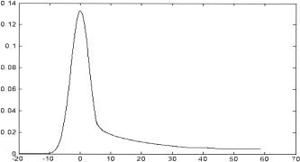
Conventional ICA models including fixed nonlinear function‐based or high‐order cumulant‐based algorithms may be unsuitable for blind separation of a variety of source distributions if the underlying assumptions on the unknown sources are violated. A better model would be able to adaptively represent any source distribution; however, it is usually hard to find a generalized model to represent both symmetric and asymmetric (skewed) source distributions. We propose two kinds of models to suitably represent symmetric and asymmetric distributions, respectively. We use the log‐Weibull (LW) distribution as a model family for skewed distributions, and model symmetric sources with three typical functions: Gaussian, Laplace, and logistic. The LW distribution is chosen as a skew modeling because conventional ICA algorithms do not work well for skewed sources [Stone et al., 2002; Suzuki et al., 2001] and LW is an asymmetric distribution with a wide coverage of variation based on simple parameters and simple high‐order cumulant computation [Silvermann, 1986]. LW is a suitable and convenient model for estimation of a variety of skewed distributions. The pdf for the LW density is written as

(1)

where the parameters a and b denote location and scale, respectively. These parameters can be calculated from the mean μ and variance σ of the random distribution. Here, b = and α≈μ−0.5772×b [Abramowitz and Stegun, 1972]. Figure 1 shows the LW distributions for various parameters.

Figure 1.

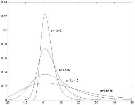
The LW distributions with different parameters.

When the data include many samples, the estimated values from data will be an approximation of real parameters. Although the true pdf of the underlying source is unknown in practical applications, it can be estimated indirectly from the reconstructed source signals that are calculated from a conventional ICA algorithm (e.g., standard Infomax ICA) using a kernel density estimation technique [Silvermann, 1986]. For a set of samples {z ₁, z ₂, …, z _N}, drawn from a random variable z, the kernel estimator is defined by

(2)

(3)

where h is the window bandwidth, chosen as 100 equally spaced points covering the range of data. This function f̂(z) is a kernel estimator of the unknown real density function f(z) with kernel function K(z). Such an estimator has been confirmed to be asymptotically unbiased and efficient as well as to converge to the real pdf as the kernel window bandwidth shrinks and the sample size grows [Silverman, 1986].

Source Density‐Driven ICA (SD‐ICA) Method

As we described above, conventional ICA may not achieve good results for certain sources when these sources seriously violate the underlying assumption. The conventional ICA algorithms, however, may provide a rough signal estimate of real sources under this situation. We can make use of the signal estimate as samples for pdf computation of the source signals so that a refitted ICA model can be found.

Let us denote x an _n‐dimensional vector of the observed mixed sources, x = (x ₁, x ₂, …, x _n)^T, which is generated by the ICA model:

(4)

where s = (s ₁, s ₂, …, s _n)^T is an _n‐dimensional vector whose elements are assumed independent sources. A _n×n is an unknown mixing matrix.

The source estimates are written as

(5)

where W _n×n is the unmixing matrix converged, and at which time ŝ is regarded as an estimate of the sources. The pdf of the estimated signal ŝ can be calculated by the kernel estimator [Silverman, 1986]

(6)

where h is the window bandwidth and z is variable. This estimated pdf is regarded as approximation for the true source pdf. A Gaussian kernel function was chosen as the density estimator K(·). The source pdf is thus estimated from the converged initial ICA signal estimates. As a consequence, the distribution parameters for different sources are calculated from the initial ICA signal estimate for all channels. These parameters are subsequently incorporated in the proposed algorithm such that an adaptive nonlinear function is used in the corresponding channel for the final source estimation stage.

SD‐ICA Algorithm

The central idea of our method is to use a three‐stage separation process with the following steps: (1) standard Infomax ICA for initial statistically independent source estimates; (2) kernel estimation for determination of the probabilistic density of these sources; and (3) source density‐based “optimal” nonlinearities for the final separation. The Infomax ICA will maximize the joint output entropy of the nonlinear function. The joint output entropy H(y) is defined as

(7)

(8)

(9)

where I(y) is the mutual information of the output y and F = (f ₁, …, f _N) is a nonlinear continuous, monotonic and multivariate function. H(y _i) is the marginal entropy of each output y _i. H(y) is expressed as

(10)

W is a weight matrix and w ₀ is a bias vector (bold lowercase letters are used herein to indicate vectors). The entropy is maximized using gradient ascent by choosing W such that

(11)

is zero, where E{ · } and p(·) denote the expectation and probabilistic density function of random variables, respectively, and f _i(·) denotes the ith nonlinear function. From equation (11), we can see that if the density of the source estimate u is proportional to or matches the corresponding derivatives of F(·), the second term will be zero. So maximizing the joint entropy H(y) is equivalent to minimizing the mutual information I(y) [Hyvärinen et al., 2001]. If the nonlinear function f _i(·) is therefore chosen to match the cumulative distribution function (CDF) of the corresponding source estimate (u _i), then optimal source separation will be achieved. In this context, optimal means a matched nonlinear function for each source.

For skewed distributions with LW modeling, the ICA weight iteration is derived from equation (11):

(12)

(13)

(14)

For different skewed sources, the corresponding parameters a and b are calculated from the ICA signal estimate u after convergence using the standard Infomax algorithm for all channels. The calculated parameters are subsequently used in the SD‐ICA algorithm such that an approximately optimal CDF is used in each corresponding channel for the final source estimation stage. The SD‐ICA weight update, unlike the existing conventional Infomax algorithms [Bell and Sejnowski, 1995; Lee et al., 1999], which uses fixed nonlinear functions, adaptively determines an optimal nonlinear function in different channels to find the best weight matrix W.

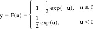
For modeling symmetric distributions, the most frequently utilized distributions are Gaussian, Laplace, and hyperbolic functions such as logistic. These three density functions are used to approximately model symmetric distributions. We can derive the ICA weight iteration algorithm based on their CDFs from equation (11). The Laplace CDF distribution as a nonlinear function is written as

(15)

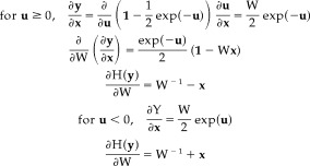
The ICA weight iterations can be derived from equation (11) and are given below:

(16)

(17)

The CDF distribution and the weight iteration of the Gaussian distribution are given below:

(18)

(19)

(20)

The weight iteration of the logistic function (equivalent to tanh function) [Bell and Sejnowski, 1995] is given by

(21)

(22)

The algorithm for the SD‐ICA framework is as follows:

• 1Preprocessing the data (e.g., whitening).
• 2Update ΔW defined in standard Infomax; stop training if weight changes below a chosen threshold.
• 3aConduct kernel density estimation on the initial “estimated” source (u = W x).
• bApply the density transformation for weighting the tail of the skewed distribution (see next section).
• cSeek the optimal‐matched nonlinear functions by minimizing the Kullback‐Leibler divergence between the original source pdf function and the estimated density function.
• 4Restart a new update ΔW according to the chosen matched nonlinear functions at the corresponding channels until convergence.
• 5If not converged, go back to step 3.

This adaptive density estimation‐driven ICA model frame is illustrated in Figure 2.

Figure 2.

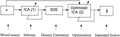
SD‐ICA model.

Density Transformation of Region of Interest

For fMRI data, the source images of interest that contain local features such as task‐related activity usually occupy a very small percentage of the total voxels. The background is less significant and can obscure the local features of interest in the activation map because conventional ICA algorithms are usually insensitive to detection of such small local features. This is because the histogram density distribution looks approximately symmetric. (i.e., the “skewness” can be hidden in the background). Figure 3a illustrates an intensity distribution of a source. To emphasize the importance of the local features of interest that are located on the tail of the distribution, some studies [Stone et al., 2002; Suzuki et al., 2001] propose a high‐order odd cumulant (e.g., third‐order) and a skewed exponential function, respectively, as the optimal nonlinear function. Although they claim that their methods improve the separation accuracy of source images for certain subjects, they still use a fixed nonlinear function and are thus not optimal for a wide variety of source distributions. Because various subjects might have different portions of local features of interest in the whole‐brain map, and even a single subject has multiple sources (e.g., task‐related, physiologic, etc.) that are likely to have different distributions, a fixed nonlinear function may not always be effective.

Figure 3.

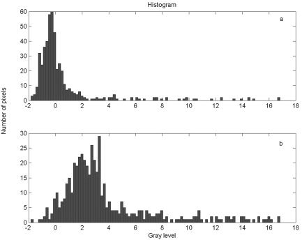
a. Histogram of an estimated signal. b. Histogram of the transformed signal.

Some conventional transformation functions (based on the gray‐level content of an entire image) such as histogram equalization and matching [Gonzalez and Woods, 2002] are suitable for overall enhancement of signals. The number of voxels of interests in the whole brain area, however, may have negligible influence on the computation of a global transformation. The first‐stage ICA algorithm is capable of telling us the location of local features (or signals) of interest, but may not detect all activated voxels. To increase and emphasize the percentage of local signals of interest across the whole brain region, a skewed histogram enhancement transformation is thus conducted on the region of interest (ROI) detected by the first‐stage ICA. Because the transformation is based on the intensity distributions of source estimates, it is adaptive for any kind of sources. The histogram transformation is

(23)

where γ is the ratio of transformation, empirically ranging from 3.0–4.0 in our case, u is a signal estimate defined in equation (9), and Tr denotes the transformation. By this transformation, the features (or signal) of interest occupy a greater ratio of the ROI and the histogram distribution is more skewed. A completely symmetric distribution, however, is almost unaffected by this transformation. Figure 3b shows the density variation of an estimated signal with this histogram transformation. Using the kernel density estimation, our SD‐ICA algorithm can adaptively determine a suitable skewed model to represent this distribution.

MATERIALS AND METHODS

Simulated Experiment

The simulation experiment is designed to test the separation of mixed synthetic sources: both symmetric and asymmetric (skewed). These sources were mixed by randomly generated full rank matrices (condition number <20). The sample size of each source in the experiment varies from 500 to 5,000 and in total, 100 independent realizations were conducted to assess reliability.

fMRI Experiment

Subjects

Eight right‐handed participants with normal vision (seven male, one female; average age, 24 years) participated in the study. The Johns Hopkins Institutional Review Board approved the protocol and all participants provided written informed consent.

Paradigms

The visual stimuli consisted of an 8‐Hz reversing checkerboard pattern presented for 15 s in the right visual cortex, and then 5 s of an asterisk fixation, 15 s of checkerboard presented to the left visual cortex, and 20 s of asterisk fixation. This set of events (55 s) was repeated four times for a total of 220 s [Calhoun, et al., 2002]. The motor paradigm required participants to touch their right thumb to each of their four fingers sequentially, back and forth, at a self‐paced rate using the hand on the same side on which the visual stimulus was presented.

Scanning parameters

Scans were acquired on a Philips NT 1.5‐Tesla scanner. A sagittal localizer scan was carried out first, followed by a T₁‐weighted anatomic scan (repeat time [TR] = 500 ms, echo time [TE] = 30 ms, field of view [FOV] = 24 cm, matrix = 256 × 256, slice thickness = 5 mm, and gap = 0.5 mm) consisting of 18 axial slices through the entire brain including most of the cerebellum. We next acquired functional scans over the same 18 slices consisting of a single‐shot, echo‐planar scan (TR = 1 s, TE = 39 ms, FOV = 24 cm, matrix = 64 × 64, slice thickness = 5 mm, gap = 0.5 mm, and flip angle = 90 degrees). Each scan run lasted 3 min 40 s and collected a total of 220 scans. Ten dummy scans were carried out at the beginning to allow for longitudinal equilibrium, after which the paradigm was automatically triggered to start by the scanner.

Data Analysis

Preprocessing

The images were first corrected for timing differences between the slice using windowed Fourier interpolation to minimize the dependence upon the chosen reference slice [Calhoun et al., 2000; van de Moortele et al., 1997]. The data were then imported into the statistical parametric mapping software package, SPM99 [Worsley and Friston, 1995]. Data were motion corrected, spatially smoothed with a 6 × 6 × 10 mm Gaussian kernel and spatially normalized into the standard space of Talairach and Tournoux [1998]. The data were slightly subsampled to 3 × 3 × 5 mm, resulting in 53 × 63 × 28 voxels.

ICA analysis

For fMRI applications, ICA can be applied spatially or temporally [Calhoun et al., 2001a]. Generally, spatial ICA has dominated the functional imaging literature so far, and in the present work we first conducted spatial Infomax ICA on the fMRI data using the Infomax algorithm [Bell and Sejnowski, 1995]. The preprocessed data from each subject were arranged into a 2D matrix of space and time and the standard spatial ICA algorithm was conducted. Principal component analysis (PCA) is often used as a data reduction step when ICA is applied to fMRI data. Twenty components were first estimated for each subject after reducing the data to this dimension via PCA. Data reduction is carried out mainly because it is assumed that there are fewer independent sources than there are time points for the spatial ICA. The minimum description length criterion was used to estimate the amount of reduction needed [Calhoun et al., 2001; McKeown et al., 1998]. The choice of 20 components is based on a reasonable tradeoff between preserving most of the variation in the data while reducing the size of the data set considerably, thus making the subsequent computations less intensive.

After applying the first ICA, the time courses and spatial maps were reconstructed for each subject. The extraction of the final components of interest is usually dependent upon a hypothetical time‐course model that is correlated with output time courses associated with the spatially independent components. ROI is obtained from the first‐stage ICA result by cropping the spatial maps of interest to remove most of the less significant background to increase the percentage of the task‐related part of the whole signal distribution. In our case, a rectangular ROI containing the occipital lobe (about one‐third of the brain) was empirically chosen. The SD‐ICA algorithm was then carried out; 10 components were estimated on the voxels within the selected ROI, and 10 components were chosen for the second‐stage ICA because the subspace (i.e., ROI) contained fewer sources. To compare the results of SD‐ICA with a conventional method, we also analyzed fMRI data using a general linear model (GLM) approach.

RESULTS

Simulated Experiment

We generated six mixed sources: Gaussian, Laplacian, sech², Rayleigh, gamma, and exponential. Results of the signal‐to‐noise ratio (SNR) measurement 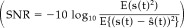show that the proposed SD‐ICA algorithm (not including the step of density transformation of ROI) has about a 10‐db gain on the separation of the skewed sources when compared to conventional ICA algorithms including Infomax [Bell and Sejnowski, 1995], extended Infomax [Lee et al., 1999], FastICA [Hyvärinen and Ojk, 1997], and JADE (joint approximate diagonalization of Eigen‐matrices) [Cardoso and Souloumiac, 1993]. For the symmetric sources, the proposed algorithm performs slightly better than do other algorithms (about 1–2 db gain) except for the sech²(·) source, for which performance is almost the same. This was expected because the proposed algorithm chooses the same ICA nonlinear function (logistic) as the standard Infomax algorithm for the sech² source. Table I shows partial performance comparison between SD‐ICA algorithm and the conventional ICA algorithms for the six mixed artificial source data. We have demonstrated that the proposed algorithm can adaptively obtain density function parameters “matching” the original source distributions, and hence improve separation performance for the mixed sources. Our simulations confirm that the proposed approach is capable of separating mixtures of a wide of variety of signals, including symmetric and asymmetric distributions, and provides superior separation performance, especially for skewed distributed sources, when compared to several existing ICA methods. Table II gives the comparison of CPU computing time for several different ICA methods. We also generated a simulation containing an fMRI‐like activation source (see Fig. 4) using this algorithm and found improved performance of SD‐ICA over conventional ICA methods.

Table I.

Performance comparison of different ICAs in blind separation

Method	Number of samples
	1,000	2,000	3,000	5,000
Rayleigh source
SD‐ICA	27.66 ± 4.4	30.69 ± 4.3	32.64 ± 4.0	35.29 ± 3.8
Infomax	18.85 ± 4.6	21.59 ± 4.4	23.52 ± 4.1	24.02 ± 3.6
Extend Infomax	19.89 ± 4.6	24.74 ± 4.5	26.33 ± 4.3	28.53 ± 4.0
JADE	21.78 ± 4.3	23.60 ± 4.3	25.92 ± 4.0	26.54 ± 3.8
FastICA (skew)	24.85 ± 4.6	26.24 ± 4.5	29.47 ± 5.1	31.16 ± 4.1
Gamma source
SD‐ICA	25.10 ± 4.3	32.68 ± 5.0	33.67 ± 4.3	36.12 ± 4.1
Infomax	17.35 ± 4.5	21.85 ± 4.4	21.68 ± 4.5	24.10 ± 3.8
Extend Infomax	17.87 ± 4.9	22.42 ± 5.2	22.54 ± 5.0	24.85 ± 4.8
JADE	17.83 ± 4.1	20.84 ± 4.3	22.22 ± 4.0	24.50 ± 3.8
FastICA (skew)	21.02 ± 5.1	25.71 ± 4.2	27.18 ± 5.7	29.25 ± 4.8
Laplacian source
SD‐ICA	34.00 ± 4.4	39.60 ± 4.3	42.20 ± 4.1	45.52 ± 3.6
Infomax	32.80 ± 4.0	37.58 ± 4.2	39.85 ± 4.0	43.30 ± 3.8
Extend Infomax	31.06 ± 4.5	35.90 ± 4.2	38.05 ± 4.3	40.95 ± 4.0
JADE	30.05 ± 4.3	34.50 ± 3.9	36.75 ± 4.2	38.20 ± 3.8
FastICA (skew)	24.56 ± 4.8	29.78 ± 4.6	31.53 ± 4.1	33.40 ± 3.6

Results from only three of six mixed sources (Laplacian, Gaussian, sech²x, Rayleigh, gamma, exponential) are given; other similar results are omitted due to space limitation. Values are given as means ± standard deviation over 100 realizations. ICA, independent component analysis; SD‐ICA, source density‐driven ICA; extend Infomax, extended Infomax; JADE, joint approximate diagonalization of Eigen‐matrices.

Table II.

Computational time comparison for different ICA methods

	SD‐ICA	Infomax	Extend Infomax	JADE	FastICA (skew)
CPU time (s)	17.50	1.969	2.281	0.2340	0.5780

Average time over 100 realizations using MATLAB script on separation of six mixed sources. ICA, independent component analysis; SD‐ICA, source density‐driven ICA; extend Infomax, extended Infomax; JADE, joint approximate diagonalization of Eigen‐matrices.

Figure 4.

A fMRI‐like activation distribution.

fMRI Experiment

Application of ICA to the fMRI activation data identifies the task‐related component. We show the results of analyzing fMRI data acquired during a visual perception task and compare a standard ICA and GLM analyses (Fig. 5). In Figure 5, we display both left and right visual cortex activation on the selected ROI. Ten components were estimated for the ICA results in the selected ROI. The regions of activation identified by the GLM seemed similar to those identified by SD‐ICA for the task‐related components in the ROI. The correlation calculation between the SD‐ICA/Infomax ICA time course and reference time‐course model shows SD‐ICA has a larger correlation value than does the Infomax ICA method. To contrast the difference between the SD‐ICA and standard ICA time courses, we compute a paired t test between the two sets of time courses on the group of eight subjects. The t test value for the right visual cortex is 3.07 (P < 0.01), showing a significant difference between the SD‐ICA and the Infomax ICA time courses. We also find a significant difference in the spatial maps (see Fig. 5 and 6) for the right visual cortex. In other words, the SD‐ICA identifies more task‐related voxels.

Figure 5.

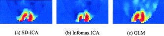
The comparison among SD‐ICA, Infomax ICA, and GLM.

Figure 6.

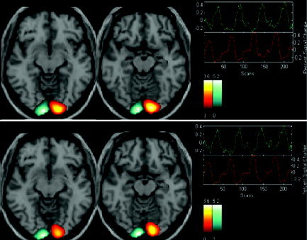
The grouped averaged ICA time courses between two ICAs. The group‐averaged correlation values with standard activation time course model are 0.9390, 0.9139 for SD‐ICA and 0.9228 and 0.8710 for Infomax ICA on the left visual and right visual cortex, respectively. Top: SD‐ICA. Bottom: Infomax ICA.

Among the applications of ICA to fMRI data, the average response across a group of subjects is particularly interesting. We use the group ICA technique [Calhoun et al., 2001b] implemented in a MATLAB toolbox [Egolf et al., 2004] and http://icatb.sourceforge.net to compare the performance of SD‐ICA and standard Infomax ICA. Figure 6 shows the comparison of these two ICA methods on a group of eight subjects. The corresponding time courses of SD‐ICA and Infomax ICA methods are also given in Figure 6, showing activation corresponding to the left cortex and right cortex stimulations. From Figure 6, we can see that SD‐ICA can achieve improved performance in terms of correlation values and spatial extent of activated brain regions compared to Infomax ICA. To demonstrate further the difference between SD‐ICA and Infomax ICA, we computed a voxel‐wise paired t test on the two task‐related images. The voxel values are calibrated to the original fMRI data and thus are in units of percent signal change [Calhoun et al., 2002; Egolf et al., 2004]. Figure 7 shows the result thresholded at P < 0.05 (t = 1.9). It demonstrates increased amplitude in visual cortex for SD‐ICA for the eight participants.

Figure 7.

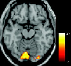
Paired t test between SD‐ICA and Infomax ICA on the group of eight subjects (t = 1.9; and P < 0.05).

DISCUSSION

ICA has great potential as a modeling tool for biomedical data. The potential of ICA methods can only be fully realized by applying additional constraints that are physiologically realistic [Stone et al., 2002; Suzuki et al., 2001]. The successful application of ICA to biomedical signals is dependent on the validity of the statistical assumptions implicit in the method. It is clear that adaptive modeling‐based ICA approach is a useful tool for understanding fMRI data. We propose a source density‐driven ICA method, aiming to embody physically realistic assumptions and thus improve optimal separation results. The performance of ICA can be improved by seeking matched nonlinearities for each source and incorporating prior information (skewed‐weighted transformation) into the ICA algorithm. We claim SD‐ICA works better than conventional ICA methods mainly because it provides for a skewed model. We incorporate skewed as well as symmetric nonlinearities into our algorithm because some work [Stone et al., 2002; Suzuki et al., 2001] has shown that task‐related fMRI activation often has a skewed distribution. SD‐ICA is thus able to represent these kinds of skewed fMRI activation signals. We also examined sensitivity and reliability measures in our experiments. For this, we conducted SD‐ICA on an individual subject (for the sensitivity test) and a group of subjects (for the reliability test). Our experiments showed that this method is more sensitive to small local features of interest and seems to provide a more accurate detection of the activated region for an individual subject. It is also useful to examine the average response across a group of subjects. For the group experiment with eight people, the SD‐ICA algorithm indicates greater spatial extent of activation than do the Infomax ICA maps for both left and right visual field simulation. For the comparison between the time courses and standard time‐course models, the SD‐ICA group‐averaged time courses have larger correlation values than does Infomax ICA for both the left and the right visual field simulation. These results show SD‐ICA improves accuracy of source separations.

The proposed SD‐ICA method can separate mixtures of both symmetric and asymmetric sources. Our simulation experiments demonstrate that SD‐ICA attempts to find matched nonlinear functions by seeking the true probability density function of each source and provides a noticeable performance improvement when compared to several existing ICA methods (standard Infomax, extended Infomax, JADE, and FastICA). From the convergence viewpoint of this algorithm, it is of relatively modest computational complexity to include the kernel density estimation and density match calculation stages. The CPU computation time comparison shows that SD‐ICA needs about 10 times as much time as the Infomax ICA algorithm. It is acceptable for SD‐ICA to conduct fMRI data analysis. In addition, it is possible for the estimated parameters of source models to be biased heavily by the first‐stage ICA for a small number of source samples. The SD‐ICA algorithm should thus be derived from a large number of source samples, where the robustness of this algorithm becomes tractable. This method is well suited for fMRI data because these data contain many samples (voxels). As discussed in Strother et al. [2002], the parameter estimation in finite data set may not be optimizable even using maximum likelihood (ML) techniques. In fMRI data analysis, it is hard to explicitly determine density parameter estimation of the underlying sources from the mixed data. To overcome bias of parameter estimation, researchers [Attias, 1999; Welling and Weber, 2001] generally use the expectation maximization (EM) algorithm based on ML to compute iterated estimates indirectly from the data. We have attempted a popular EM algorithm [Welling and Weber, 2001] on fMRI data, but found series convergence problem. The assessment of this bias is thus not easy for real data. More work is needed to understand the impact of bias and variance tradeoff for SD‐ICA and other ICA algorithms in fMRI data analysis.

In fMRI studies, the interesting target of analysis typically occupies a small percentage of the total number of voxels. To improve efficiency, the analysis can be restricted to a specific ROI. There are at least three ways to generate this ROI: (1) define a large rectangular region inclusive of cortex (e.g., using Talairach coordinate system [Talairach and Tournoux, 1998]); (2) a cortex‐based ROI that includes only those voxels that lie within the cortex (approximate 20% of the total) [Formisano et al., 2001]; or (3) an ICA‐based ROI (used in the present work) in which the ROI is obtained from the first‐stage ICA result by cropping the spatial maps of interest to remove most of the less significant background for increasing the percentage of the task‐related part of the whole signal distribution (e.g., x = 15–41, y = 1–5, and z = 6–13; see single‐slice image in Fig. 5). In our case, a rectangular ROI containing the occipital lobe was chosen empirically (incorporating about one‐third of the brain). Besides reducing computational demands, using a ROI approach increases the relative contribution of the activated regions (relative to the background of, e.g., white matter) and hence improves the ICA performance.

In summary, we have shown that the SD‐ICA approach improves the fitting of the ICA model for fMRI data. In addition, using simulations, we show that the SD‐ICA algorithm outperforms other ICA algorithms such as Infomax, JADE, and FastICA in blind source separation. We have demonstrated that the SD‐ICA approach, although slightly increasing the computational load, improves the performance of the source separation and may prove a useful addition to existing techniques for fMRI data analysis.

The joint output entropy is defined by Bell and Sejnowski [1995] as

(24)

where I(y), is the mutual information of the output y, H y _i, is the marginal entropy of each output y _i.

(25)

(26)

The entropy is maximized using gradient ascent by choosing W such that

(27)

is zero. The Infomax ICA weight update is

(28)

The cumulative distribution function of Laplace distributions are written as

(29)

Without loss of generalization, we assume (μ = 0, σ = 1), and then the nonlinear function is written by

(30)

So we have

(31)

For skewed distributions, the log‐Weibull‐based ICA weight update algorithm is derived below,

(32)

So we have

(33)

REFERENCES

- Abramowitz M, Stegun IA, editors (1972): Handbook of mathematical functions with formulas, graphs, and mathematical tables. New York: Dover. [Google Scholar]
- Attias H (1999): Independent factor analysis. Neural Comput 11: 803–851. [DOI] [PubMed] [Google Scholar]
- Bach F, Jordan M (2002): Kernel independent component analysis. J Mach Learn Res 3: 1–48. [Google Scholar]
- Bell A, Sejnowski TJ (1995): An information–maximizing approach to blind separation and blind separation and blind deconvolution. Neural Comput 7: 1129–1159. [DOI] [PubMed] [Google Scholar]
- Biswal BB, Ulmer JL (1999): Blind source separation of multiple signal sources of fMRI data sets using independent component analysis, J Comput Assist Tomogr 23: 265–271. [DOI] [PubMed] [Google Scholar]
- Calhoun VD, Adali T, Pearlson GD, Pekar JJ (2001a): Spatial and temporal independent component analysis of functional MRI data containing a pair of task‐related waveforms. Hum Brain Mapp 13: 43–53. [DOI] [PMC free article] [PubMed] [Google Scholar]
- Calhoun VD, Adali T, Pearlson GD, Pekar JJ (2001b): A method for making group inferences from functional MRI data using independent component analysis. Hum Brain Mapp 14: 140–150. [DOI] [PMC free article] [PubMed] [Google Scholar]
- Calhoun VD, Adali T, Pearlson GD, Pekar JJ (2001c): Group ICA of functional MRI data: separability, stationarity and inference. Proceedings of the International Conference on Independent Component Analysis and Blind Signal Separation. San Diego, CA. p 155–160.
- Calhoun VD, Golay X, Pearlson GD (2000): Improved FMRI slice timing correction: Interpolation errors and wrap around effects. Proceedings of the ISMRM 9th Annual Meeting. Denver, USA.
- Calhoun VD, Pekar JJ, McGinty VB, Adali, T , Watson, TD , Pearlson GD (2002): Different activation dynamics in multiple neural systems during simulated driving. Hum Brain Mapp 16: 158–167. [DOI] [PMC free article] [PubMed] [Google Scholar]
- Cardoso JF, Souloumiac A (1993): Blind beamforming for non‐Gaussian signals. IEE Proc F 140: 362–370. [Google Scholar]
- Cardoso JF (1998): Blind signal separation: statistical principles. Proc IEEE 86: 2009–2025. [Google Scholar]
- Dodel S, Herrmann JM, Geisel T (2000): Localization of brain activity—blind separation for fMRI data. Neurocomputing 32: 701–708. [Google Scholar]
- Egolf E, Kiehl KA, Calhoun VD (2004): Group ICA of fMRI toolbox (GIFT). Society of Biological Psychiatry's 59th Annual Scientific Convention and Program. New York, NY.
- Gonzalez R, Woods R (2002): Digital image processing. UK: Pearson Education, Inc. [Google Scholar]
- Formisano E, Esposito F, Salle FD, Goebel R (2001): Cortex‐based independent component analysis of fMRI time‐series. Neuroimage 13(Suppl.): 119. [DOI] [PubMed] [Google Scholar]
- Hyvärinen A, Karhunen J, Oja E (2001): Independent component analysis. New York: John Wiley & Sons, Inc. 504 p. [Google Scholar]
- Hyvärinen A, Ojk, E (1997): A fast fixed‐point algorithms for independent component analysis. Neural Comput 9: 1483–1492. [DOI] [PubMed] [Google Scholar]
- Lee TW, Girolami M, Sejnowski TJ (1999): Independent component analysis using an extended Infomax algorithm for subgaussian and supergaussian sources. Neural Comput 11: 417–441. [DOI] [PubMed] [Google Scholar]
- McKeown MJ (2000): Detection of consistently task‐related activations in fMRI data with hybrid independent component analysis. Neuroimage 11: 24–35. [DOI] [PubMed] [Google Scholar]
- McKeown MJ, Makeig S, Brown GG, Jung TP, Kinderman, SS , Bell AJ, Sejnowski TJ (1998): Analysis of fMRI data by blind separation into independent spatial components. Hum Brain Mapp 6: 160–188. [DOI] [PMC free article] [PubMed] [Google Scholar]
- McKeown MJ, Sejnowski TJ (1998): Independent component analysis of fMRI data: examining the assumptions. Hum Brain Mapp 6: 368–372. [DOI] [PMC free article] [PubMed] [Google Scholar]
- Nakada T, Suzuki K, Fujii Y, Matsuzawa H, Kwee IL (2000): Independent component‐cross correlation‐sequential epoch (ICS) analysis of high field FMRI time series: direct visualization of dual representation of the primary motor cortex in human. Neurosci Res 37: 237–244. [DOI] [PubMed] [Google Scholar]
- Porrill J, Stone JV, Berwick J, Mayhew J, Coffey P (2000): Analysis of optimal imaging data using weak models and ICA In: Giromi M, editor. Advances in independent component analysis. New York: Springer‐Verlag; p 217–233. [Google Scholar]
- Silvermann BW (1986): Density estimation for statistics and data analysis. New York: Chapman & Hall; 176 p. [Google Scholar]
- Stone JV, Porrill J, Porter NR, Wilkinson ID (2002): Spatiotemporal independent component analysis of event‐related fMRI data using skewed probability density functions. Neuroimage 15: 407–421. [DOI] [PubMed] [Google Scholar]
- Strother SC, Anderson J, Hansen LK, Kjems U, Kustra R, Sidtis J, Frutiger S, Muley S, LaConte S, Rottenberg D (2002): The quantitative evaluation of functional neuroimaging experiments: the NPAIRS data analysis framework. Neuroimage 15: 747–771. [DOI] [PubMed] [Google Scholar]
- Suzuki K, Kiryu T, Nakada T (2001): Fast precise independent component analysis for high field fMRI time series tailored using a prior information on spatiotemporal structure. Hum Brain Mapp 15: 54–66. [DOI] [PMC free article] [PubMed] [Google Scholar]
- Talairach J, Tournoux P (1998): Co‐planar stereotaxic atlas of the human brain. Thieme: Stuttgart. [Google Scholar]
- van de Moortele PF, Cerf B, Lobel E, Paradis AL, Faurion A, Le Bihan D (1997): Latencies in fMRI time‐series: effect of slice acquisition order and perception. NMR Biomed 10: 230–236. [DOI] [PubMed] [Google Scholar]
- Vlassis N, Motomura Y (2001): Efficient source adaptivity in independent component analysis. IEEE Trans Neural Netw 12: 559–566. [DOI] [PubMed] [Google Scholar]
- Welling M, Weber M (2001): A constrained EM algorithm for independent component analysis. Neural Comput 13: 677–689. [DOI] [PubMed] [Google Scholar]
- Worsley KJ, Friston KJ (1995): Analysis of fMRI time‐series revisited‐again. Neuroimage 2: 173–181. [DOI] [PubMed] [Google Scholar]