

Abstract
Simultaneous electroencephalography (EEG) and functional magnetic resonance imaging (fMRI) may allow functional imaging of the brain at high temporal and spatial resolution. Artifacts generated in the EEG signal during MR acquisition, however, continue to pose a major challenge. Due to these artifacts, an interleaved modus has often been used for “evoked potential” experiments, i.e., only EEG signals recorded between MRI scan periods were assessed. An obvious disadvantage of this approach is the loss of a portion of the EEG information, which might be relevant for the specific scientific issue. In this study, continuous, simultaneous EEG‐fMRI measurements were carried out. Visual evoked potentials (VEPs) could be reconstructed reliably from periods during MR scanning and in between successive scans. No significant differences between both VEPs were detected. This indicates sufficient artifact removal as well as physiological correspondence of VEPs in both periods. Simultaneous continuous VEP‐fMRI recordings are thus shown to be feasible. Hum Brain Mapp, 2005. © 2005 Wiley‐Liss, Inc.
Keywords: electroencephalography, simultaneous EEG‐fMRI, functional brain imaging, artifact removal, visual evoked potentials
INTRODUCTION
Simultaneous electroencephalography (EEG) and functional magnetic resonance imaging (fMRI) is becoming increasingly attractive in neuroscience due to the complementary properties of the two techniques. Although EEG provides a high temporal resolution measure of synchronous synaptic activity, fMRI makes anatomical localization of neuronal activity associated blood oxygen level‐dependent (BOLD) signal possible at a millimeter‐level spatial resolution. Provided that the measured EEG signal measures net synaptic activity changes and not merely a change in synaptic synchronization and that the BOLD signal reflects synaptic activity changes as well, a combination of both methods could noninvasively localize synaptic activity changes in both space and time. The major obstacles in implementing simultaneous EEG‐fMRI, however, are the strong artifacts in the EEG signal that are induced by the magnetic field of the fMRI. One artifact called the cardioballistic artifact depends on the high static magnetic (B0) field [Allen et al., 1998; Kim et al., 2004], another artifact is due to the switching of radiofrequency (RF) pulses and magnetic field gradients [Allen et al., 2000]. It is generally thought that the cardioballistic artifact arises mainly from arterial pulse‐associated movements of the electrodes in the B0‐field [Anami et al., 2003] and possibly to a lesser degree from electromotive force of blood ions [Bonmassar et al., 2002; Ellingson et al., 2004; Kim et al., 2004]. The precise contribution of each component, however, is not yet fully known. The amplitudes of this artifact are on the order of normal EEG amplitudes and the main frequency components lie between 4 and 7 Hz. It occurs with the heartbeat frequency (around 1 Hz). Although a nuisance, this time‐ and frequency‐limited artifact leaves the EEG recognizable and utilizable for most purposes. The second class of artifacts arising from RF pulses and gradients is much more problematic. These artifacts, which occur during fMRI acquisition periods, have a wide frequency range and huge amplitudes of several millivolts, making the EEG (with amplitudes around 10–250 μV) unrecognizable. This is why earlier combined EEG‐fMRI studies [Babiloni et al., 2002; Bonmassar et al., 1999, 2001; Christmann et al., 2002; Goldman et al., 2002; Kruggel et al., 2000, 2001; Sommer et al., 2003; Thees et al., 2003] discarded the artifact‐contaminated segments and used only EEG ‐periods between two successive MRI scans (“interleaved” EEG‐fMRI). The obvious disadvantage of this approach is that one loses potentially valuable EEG information during MR scan periods. In addition, interleaved acquisition is often more time consuming, which is a problem in evoked potential studies that require averaging over many trials. In particular, studies of nonauditory evoked potentials would benefit from simultaneous measurements, as these potentials can also be collected in the non‐silent (acquisition) periods and not only between MRI scans (the silent period).
With the advent of high‐dynamic‐range amplifiers that can capture the full range of amplitudes including those of the fMRI artifacts, it turned out that the shape of these artifacts is almost constant over time. It was therefore tested whether one could eliminate artifacts from the EEG signal by subtracting an artifact template, which is a weighted average of all artifact periods [Allen et al., 2000]. This is only possible if these artifacts add linearly to the actual EEG signal. Recently, this artifact correction algorithm was used to reconstruct EEG signals that revealed α‐rhythm modulation and epileptic activity [Laufs et al., 2003; Moosmann et al., 2003; Salek‐Haddadi et al., 2002].
Epileptic activity and the α rhythm, however, are entities whose parameters are variable and not predictable. A better‐defined reference signal with constant amplitude or latency would be desirable for estimating the quality of the artifact‐corrected signal. Reproducibility and predictability of the physiological signal, as it holds for evoked potentials, is required for investigating the equivalence of evoked responses. Until now, it was uncertain whether evoked potentials that have smaller amplitudes than epileptic activity does and a more complex shape than that of the α rhythm can be reconstructed from artifact‐contaminated EEG signals. To the best of our knowledge, we present here the first continuous, simultaneous EEG‐fMRI study to systematically compare visual evoked potentials (VEPs) recorded during interscan periods to those recorded during MRI scan periods after application of an artifact‐removal algorithm. Whether it is possible to extract physiological event‐related potential (ERP) signals from scan periods is highly relevant for truly simultaneous acquisition of ERPs and fMRI, particularly in MRI acquisition with short interscan intervals or in experimental designs that overlap the stimulation and acquisition periods. The success of the artifact‐removal algorithm would also open the door to investigating the relationship between single‐trial electrical responses and their vascular correlates.
MATERIALS AND METHODS
MRI Data Acquisition
MRI measurements were carried out on a 1.5‐T whole body scanner (Magnetom Vision; Siemens, Erlangen, Germany) using a standard head‐coil in our laboratory at the Division of Neuroimaging, Charité and the Berlin NeuroImaging Center. To minimize susceptibility distortions due to local static magnetic field inhomogeneities, an automatic shimming procedure was applied. For each subject, an anatomical volume data set was acquired using a T1‐weighted 3D‐magnetization prepared rapid acquisition gradient echo (MPRAGE) sequence (repetition time [TR] = 94 msec, echo time [TE] = 4 msec, flip angle = 12 degrees, and voxel size = 1 × 1 × 1 mm3). Functional imaging was carried out using a T2*‐weighted BOLD [Bandettini et al., 1992; Frahm et al., 1992; Kwong et al., 1992; Ogawa et al., 1992] sensitive gradient echo planar imaging sequence. The fMRI parameters were TE = 60 msec, flip angle = 90 degrees, matrix = 64 × 64, voxel size = 3.3 × 3.3 × 5 mm3, TR = 4.2 sec, acquisition time = 2,100 msec, interslice distance = 0.5 mm, and 20 slices; 120 scans were acquired in each volunteer.
EEG recording
For EEG‐recordings, we used an MR‐compatible 32‐channel‐amplifier (BrainAmp; Brain Products Inc., Munich, Germany; 5‐kHz sampling rate) and an MR‐compatible EEG cap (Easy‐Cap; FMS, Herrsching‐Breitbrunn, Germany) with 29 ring‐type sintered AgCl electrodes with iron‐free copper leads twisted pairwise, arranged according to the International 10‐20 System, referenced against an electrode centered between Cz and Fz. Electrode‐skin impedance for all electrodes was maintained to be ≤10 kΩ by applying an electrode paste (ABRALYT 2000; FMS, Herrsching‐Breitbrunn, Germany). To avoid movement‐related EEG artifacts, the head was fixed in the head‐coil by a vacuum pad, and heavy sandbags immobilized the electrode leads. An electrooculogram (EOG) and an electrocardiogram (ECG) were also recorded. The amplifier was placed behind the subject's head in the bore of the scanner. A fiberoptic cable connected the amplifier to a standard EEG PC in the MR console room running Vision Recorder Software v1.02 (Brain Products Inc., Munich, Germany). Resolution of the amplifier was 500 nV. A preamplifier analogue high‐cutoff filter of 250 Hz was applied for reducing amplitudes of the high‐frequency artifact components before amplification to avoid saturation of the recorded signal.
Paradigm and Experimental Design
Five healthy subjects (females; mean age ± standard deviation [SD] = 26.75 ± 2.50 years; age range = 23–30 years) with normal or corrected‐to‐normal vision participated in the study. Written informed consent was obtained according to the declaration of Helsinki. Subjects were asked to fixate on the fixation cross of the stimulus and to avoid any movements or excessive eye blinks during the whole experiment. While lying in the bore of the scanner, subjects watched the visual stimulus via a mirror above their heads, reflecting the image from a screen attached to the head‐coil. The stimulus was projected onto the acrylic screen through a collimating lens by a conventional video projector, which was placed about 4 m from the isocenter of the MR scanner. A black‐and‐white circular checkerboard (field size adjusted to magnification factors of the retinocortical representation) with a central fixation cross was presented and contrast reversed once during an acquisition period (when the large MRI artifact superimposes itself onto the EEG signal) and once during the non‐acquisition period, each lasting 2.1 sec (Fig. 1). The stimulus sequence was programmed using the software Presentation v0.71 (Neurobehavioral Systems, Albany, NY). The MRI scanner triggered the stimulus computer. Two constraints were given for the stimulus timing: (1) one stimulus was to be presented during scan and interscan intervals, respectively; and (2) stimulation was to start at least 1,000 msec (length of the average VEP) before the next switch between scan/interscan period so as to assign each VEP clearly to either a scan or an interscan period. Within these constraints, interstimulus intervals (ISIs) were variable and randomized. For each subject, 120 scans were recorded, comprising 120 trials within the artifact period and 120 trials within the non‐artifact period.
Figure 1.
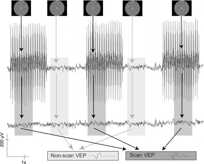
Experimental design: checkerboard‐stimuli were presented once in each scan and non‐scan interval. After artifact correction, visual evoked potentials (VEPs) were calculated by respective averaging of scan and non‐scan epochs.
A slightly modified version of the above‐mentioned design was optimized for distinct BOLD response modulation and used in one subject to examine paradigm‐correlated functional MR images. The only difference was the insertion of resting periods after each 10 sec of stimulation lasting for 10 sec, during which no visual stimuli were presented, to allow for a sufficient modulation of the BOLD response.
Data Analysis
Functional MRI artifact detection and correction
Using Vision Analyzer software (Brain Products Inc.) the onsets of fMRI artifact periods in the EEG signal were identified by the immediate occurrence of high‐amplitude artifacts. Because MR artifact patterns are supposedly constant in time and add linearly to the EEG signal, the signal was corrected by subtracting weighted moving averages of (scan‐wise) artifact epochs, using the same formula used by Allen et al. [2000]. The exact artifact correction algorithm works as described below.
-
1
Epochs of 4.2‐sec length including both scan and interscan periods (An is an epoch comprising one scan and interscan period) are segmented based on the onset of MR artifacts. Epochs are baseline corrected using a time window of 20–5 msec before MR acquisition onset. To correct for small temporal shifts between artifacts due to a limited sampling frequency of 5 kHz, epochs are interpolated up to 50 kHz (cubic spline method, MATLAB; The MathWorks Inc., Natick, MA) and subsequently aligned by maximizing cross correlation. After phase correction, epochs are downsampled to the original sampling frequency of 5 kHz.
-
2In Equation (1), an individual (per epoch) artifact template Bn (n = epoch index) is created for each epoch An by calculating a weighted average w|n − i| of all epochs (k = number of epochs; here k = 120) with the parameter w = 0.9 providing an exponential decay, resulting in stronger weights for nearby artifacts and thus accounting for possible changes of the artifact over time. Because physiological signatures of the EEG are not time locked to the beginning of each epoch, the average of these signals tend toward zero and only the artifacts remain.

(1) -
3In Equation (2), individual templates Bn are subtracted from respective artifact periods An to give Cn, the artifact‐corrected epoch.

(2)
EEG data analysis and evoked potential analysis
Analysis was carried out using MATLAB v.6.1. After MR artifact correction, a bandpass filter of 0.53–70 Hz (Butterworth; zero phase distortion) was applied. Data from stimulus epochs were segmented and baseline corrected. VEPs were calculated by respective averaging of scan and interscan single‐trial responses (no epochs were discarded after visual inspection for movement artifacts) from electrode O2 (n = 120 each; Fig. 1). In one subject, four VEPs, each comprising 120 trials, were acquired without concurrent MR acquisition to obtain a reference measure of physiological VEP variance.
Although no prominent ballistocardiograms were visible in the EEG, we determined the effect of ballistocardiogram correction in one subject. For ballistocardiogram removal, we employed an algorithm provided by Brain Analyzer software (Brain Products, Inc.), which is based on electrocardiogram‐guided artifact identification and subsequent template subtraction similar to the MR artifact correction procedure described above. Because no improvement was achieved, ballistocardiogram removal was not carried out in subsequent data analysis (Fig. 2).
Figure 2.
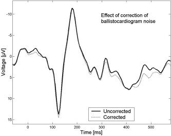
Visual evoked potentials (VEPs) are highly concordant before and after ballistocardiogram correction (data of one representative subject shown).
To reveal intraindividual differences in the structural VEP features (P2/N3 complex), latencies and amplitudes of the P2 and the N3 components were calculated and compared. Amplitudes and latencies of all five subjects were examined for significant differences between the two conditions by application of the Wilcoxon signed‐rank test (for paired samples). In addition, a correlation analysis between scan and interscan P2/N3 complexes of each subject was carried out (Fig. 3, highlighted interval). Furthermore, signal‐to‐noise ratios (SNRs) of the VEP in both conditions were estimated. Noise power was defined as the average squared difference between VEP and single‐trial response. Signal power was defined as the difference of the across‐trial average squared amplitude (whole power) and noise power. The ratio was determined by dividing signal power by noise power.
Figure 3.
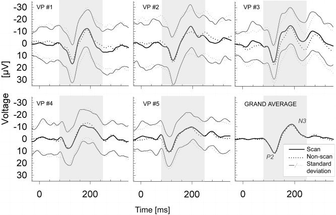
Single‐subject averages for all five subjects and grand average of all subjects (bottom right) for scan (solid line) and non‐scan (dashed line) periods. Highlighted periods were included in correlation analysis.
Evaluation of artifact‐removal algorithm
To assess the quality of artifact removal, we carried out a spectral analysis of the artifact‐free raw EEG data and the corrected EEG signal (both bandpass filtered and downsampled to 200 Hz). We estimated percentage differences in the spectral density of five frequency bands (0.6–4.3 Hz, 4.3–8 Hz, 8–12.2 Hz, 12.2–25 Hz, and 25–44 Hz) by applying the same formula as that used in Allen et al. [2000]:
where PNS is the power spectral density of non‐scan periods and PS is the power spectral density of scan periods. This was done for channel O2 in each subject and the median of these values (across subjects) was calculated.
We also analyzed the noise cancellation effect inherent in averaging for scan and non‐scan trials by calculating spectral densities as a function of the number of averaged trials. This was done for the physiologically relevant low‐frequency range of 1–45 Hz as well as for the high‐frequency range of 50–2,500 Hz. The above‐mentioned SNR should also indicate the success of artifact removal because residual artifact components would systematically worsen this ratio.
fMRI data analysis
Analysis of fMRI data consisted of preprocessing and calculation of statistical parametric maps using SPM2 (http://www.fil.ion.ucl.ac.uk/spm/spm2b.html). Preprocessing included realignment, normalization of the anatomical and functional data to the Montreal Neurological Institute (MNI) standard brain, and spatial smoothing of the functional images with a 3D Gaussian filter with a full‐width half‐maximum (FWHM) of double voxel size.
RESULTS
VEPs
Typically configured, reproducible VEPs in the form of a P2/N3 complex were found in all subjects and all runs. Single‐subject results and the grand average are given in Figure 2. The temporal characteristics of the peak responses (P2 and N3) were consistent across subjects and peak‐to‐peak amplitudes were of similar size (see Table I). No significant differences were revealed by the (two‐tailed) paired Wilcoxon signed‐rank test [Glantz, 1997] for P2/N3 latencies or for P2/N3 peak‐to‐peak amplitudes of the two conditions (scan phase vs. non‐scan phase; α ≤ 0.062; due to its discrete nature, only an approximation of the usual α value of 0.05 can be achieved). The statistical power of this test was calculated by estimating the power of the analogous t test (matched pairs), discounting 5% [Glantz, 1997]. This provides a statistical power of 0.9 for an assumed “true” difference of latencies of >4 msec for the P2 latency and a P2–N3 amplitude difference of >5 μV between groups. Standard deviation (SD) at each time point and explicitly calculated SNRs were similar for both conditions (Table I). Blinks or movement artifacts did not compromise the averaged VEP; thus all trials were included into the VEP average.
Table I.
Peak‐to‐peak amplitudes, latencies, standard deviations, and correlation coefficients of P2/N3 complex
| Subject no. | Parameter | MR Scan | Non‐scan |
|---|---|---|---|
| 1 | Latency P2 (msec) | 129 | 130 |
| Latency N3 (msec) | 187 | 186 | |
| Amplitude P2N3 (μV) | 30 | 25 | |
| Mean of SD (μV) | 15 | 16 | |
| SNR | 0.07 | 0.04 | |
| CC P2N3 | 0.99 | ||
| 2 | Latency P2 (msec) | 124 | 124 |
| Latency N3 (msec) | 193 | 194 | |
| Amplitude P2N3 (μV) | 29 | 26 | |
| Mean of SD (μV) | 13 | 13 | |
| SNR | 0.06 | 0.05 | |
| CC P2N3 | 0.98 | ||
| 3 | Latency P2 (msec) | 121 | 122 |
| Latency N3 (msec) | 185 | 186 | |
| Amplitude P2N3 (μV) | 31 | 32 | |
| Mean of SD (μV) | 17 | 20 | |
| SNR | 0.07 | 0.08 | |
| CC P2N3 | 0.98 | ||
| 4 | Latency P2 (msec) | 113 | 117 |
| Latency N3 (msec) | 173 | 189 | |
| Amplitude P2N3 (μV) | 19 | 21 | |
| Mean of SD (μV) | 14 | 15 | |
| SNR | 0.04 | 0.06 | |
| CC P2N3 | 0.99 | ||
| 5 | Latency P2 (msec) | 111 | 111 |
| Latency N3 (msec) | 198 | 196 | |
| Amplitude P2N3 (μV) | 21 | 21 | |
| Mean of SD (μV) | 11 | 11 | |
| SNR | 0.09 | 0.06 | |
| CC P2N3 | 0.99 | ||
| Reference | Mean Latency P2 (msec) | 107 ± 1 | |
| Mean Latency N3 (msec) | 183 ± 11 | ||
| Mean amplitude P2N3 (μV) | 22 ± 1 | ||
| Mean of SD (μV) | 13 ± 1 | ||
| SNR | 0.07 ± 0.01 | ||
| Mean CC P2N3 | 0.988 ± 0.003 | ||
| Mean | Latency P2 (msec) | 122 | 123 |
| Latency N3 (msec) | 189 | 188 | |
| Amplitude P2N3 (μV) | 24 | 23 | |
| SNR | 0.07 | 0.06 | |
| CC P2N3 | 0.99 | ||
Peak‐to‐peak amplitudes, latencies, standard deviation (SD; averaged over P2N3 interval) of single‐trial electrical activity from visual evoked potential, correlation coefficients (CC), and signal‐to‐noise ratios (SNR) of P2/N3 complex for all subjects and conditions, including a reference subject recorded outside the scanner.
A robust correlation of 0.98–0.99 was found between both groups of VEPs in all subjects (within the interval of P2/N3 components), comparable to the correlations found between the MR artifact‐unafflicted VEPs in the reference subject (Table I). Differences between scan and non‐scan periods seemed to lie within the natural variance given by the standard deviation of the reference subject (for visual inspection, see Fig. 4).
Figure 4.
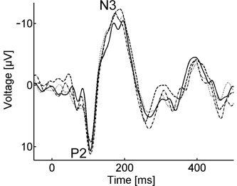
Four visual evoked potentials (VEPs), each averaged over 120 trials, recorded outside the scanner from one single subject during one session under identical environmental conditions.
Frequency Analysis
Using fast Fourier transformation, power spectral densities were calculated for artifact‐distorted, artifact‐corrected, and artifact‐free data. For the artifact‐distorted raw data, especially strong high‐frequency components were observed. These components and their harmonics completely dominate the frequency spectrum; however, artifacts might also distort lower frequency bands. Our results show that artifact‐corrected data have a frequency spectrum similar to the spectrum of the artifact‐free non‐scan (B0) data. Median percentage differences were as follows: 0.6–4.3 Hz, 8%; 4.3–8 Hz, 8%; 8–12.2 Hz, 9%; 12.2–25 Hz, 8%; and 25–44 Hz, 7%. Residual artifacts remain in the frequency range above 100 Hz in the absence of low‐pass filtering. These residual components are one order of magnitude smaller than that in the uncorrected data. Spectral power densities in this high‐frequency range are depicted in Figure 5 (top right) for artifact‐corrected unfiltered data from scan periods. For the physiologically more relevant frequency range of 1–45 Hz, power spectra are shown for non‐scan as well as scan periods in Figure 5 (left). In this figure the effect of noise cancellation for non‐phase‐locked components is visualized, spectra are depicted as a function of the averaged trial number. For small numbers of averaged trials and for the final VEP average, spectra of scan and non‐scan conditions are similar. This indicates that no significant MR artifact residuals are present after artifact correction in this frequency range. In contrast, strong artifact residuals are present in the high‐frequency range in scan but not in non‐scan data (non‐scan data not shown).
Figure 5.
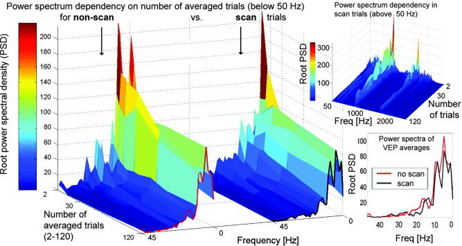
Power spectrum dependency on the number of averaged trials for the physiologically relevant frequency range of 1–45 Hz for non‐scan and scan trials (left side) and high‐frequency range of 50–2,500 Hz for scan trials (top right) for one representative subject. For better comparability, power spectra for final VEPs (n = 120) are depicted at bottom right.
Functional MRI Data Set
As expected, fMRI data (Subject 5; Fig. 6) show that visual areas of the occipital cortex are activated, primarily visual areas V1 and V2. The electrophysiological response of Subject 5 matches the pattern found in the other subjects with the standard paradigm.
Figure 6.
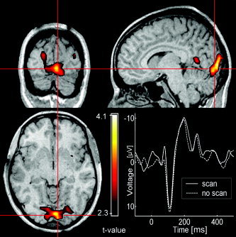
Statistical analysis of fMRI data in Subject 5 shows activations (P < 0.01) in occipital visual areas, primarily in areas V1 and V2. The respective scan‐ and non‐scan visual evoked potentials (VEPs) of Subject 5 are depicted.
DISCUSSION
We employed checkerboard visual stimulation to investigate whether VEPs can be acquired from MRI scan periods. VEPs elicited by a checkerboard have the advantage of well‐defined structural features. Other groups have already addressed the question whether VEPs recorded in the B0 field of the MR scanner are similar to those recorded outside the magnetic field of the scanner. Latencies of VEPs in interscan periods and outside the scanner are not significantly different [Bonmassar et al., 1999; Kruggel et al., 2000; Sommer et al., 2003]. In this study, we asked the question of whether there are differences between VEPs recorded during artifact‐distorted scan periods versus VEPs recorded during interscan periods.
To a first approximation, subtractive artifact removal seems to be a reasonable approach to simultaneous VEP‐fMRI measurements. No systematic differences were found between interscan and scan VEPs after artifact removal in latency, amplitude of the main component, or in the general shape of the evoked potentials, as indicated by the high correlation coefficients between both VEP groups. Nevertheless, some minor differences were seen in individual subjects. Given the known variability of VEPs even without exposure to artifacts, particularly in amplitude, as can be seen in Figure 4, these differences between scan and non‐scan periods seem to lie within the range of such natural variance. Any systematic effects of the MRI scan fell below the detection limit of this pilot study. As VEPs have relatively high amplitudes (of 20–30 μV peak‐to‐peak), a visual paradigm was chosen as a starting point for recovering information about evoked electrical activity. Our results not only indicate sufficient artifact correction but also suggest that the physiological processes underlying VEP generation are not altered significantly during MRI acquisition.
Statistics
Different strategies have been employed for the comparison of evoked potentials. Visual inspection is often sufficient [Bonmassar et al., 2002; Felblinger et al., 1999]. For statistical evaluation, the Kruskal‐Wallis test, which tests for differences between conditions inter‐individually, can be employed [Kruggel et al., 2000; Muri et al., 1998]. This test is a nonparametric analogue of the parametric analysis of variance (ANOVA). It is used for multiple comparisons between subjects; however, it has fewer assumptions about the data (no normal distribution or homogenous variances are necessary). Here, we used an intraindividual, nonparametric, rank‐based test for the statistical comparison of VEPs recorded with concurrent MR acquisition versus that recorded without concurrent MR acquisition. As there are repeated measures and only two conditions, a paired rank‐based test for single comparison is suitable. In the case of a normal distribution, the Wilcoxon signed‐rank test has approximately 95–96% of the power of an analogous paired t test [Glantz, 1997]. The application of a t test is only robust for deviations from the normal distribution if the number of pairs exceeds 10 [Sachs, 1993]. Because in this study only five pairs were evaluated, a rank‐based test was considered most appropriate. No inferences regarding N3 latency can be drawn, since due to the relatively high variance of this component the test power is relatively poor (Fig 4). Larger subject numbers are required to increase the test power sufficiently. The results of the correlation analysis, however, support the hypothesis that the visual evoked P2‐N3 complex is equivalent under both conditions.
Cardioballistic and Movement Artifacts
In contrast to former studies, cardioballistic artifacts here were of minor importance. In our experience, this is due to the tight fixation of the electrodes within the EEG cap (see discussion in Moosmann et al. [2003]. It is not clear, however, whether the minor high frequency residual artifacts observable in the power spectrum of the unfiltered raw data are due to the subjects' movements or other factors that produce slight variations of the artifact not eliminated by subtraction of a template. Certainly, the removal will need to be optimized before one can confidently reconstruct physiological EEG data in these high‐frequency bands.
Spectral Analysis and Implications for Nonvisual ERPs
Considering the results of the spectral analysis, it has become clear that high‐frequency artifact residuals remain present to a nonnegligible degree. Because these artifacts are not time‐locked to the stimulus onset (depending on experimental design), they may be overcome by sufficient averaging and possibly low‐pass filtering (as seen in the data presented here). Many ERP studies can therefore benefit from algorithms such as the one presented here.
Outlook and Benefits
EEG has limitations in localizing sources of brain electric activity due to the nonexistence of a unique solution to the EEG inverse problem [Balish and Muratore, 1990; Koles, 1998, Musha and Okamoto, 1999]. Simultaneous fMRI‐EEG recording can add spatial resolution and may help to find plausible solutions for the inverse problem and thus improve dipole fitting. Other potential benefits of simultaneous fMRI‐EEG recordings include the following: (1) no differences in cognitive strategies that could confound the results (of separate measurements); (2) equal environmental factors; (3) no training effects that occur when doing two measurements in succession; and (4) less time needed for many (nonauditory) studies. It is only possible to take full advantage of these benefits, however, when EEG (and evoked potentials) and MRI signals can be measured and analyzed continuously without loss of physiological information. This improvement may help to increase flexibility in experimental designs and thus enlarge the range and scope of functional imaging studies.
Acknowledgements
We thank Dr. Martin Stemmler for helpful comments.
REFERENCES
- Allen PJ, Josephs O, Turner R (2000): A method for removing imaging artifact from continuous EEG recorded during functional MRI. Neuroimage 12: 230–239. [DOI] [PubMed] [Google Scholar]
- Allen PJ, Polizzi G, Krakow K, Fish DR, Lemieux L (1998): Identification of EEG events in the MR scanner: the problem of pulse artifact and a method for its subtraction. Neuroimage 8: 229–239. [DOI] [PubMed] [Google Scholar]
- Anami K, Mori T, Tanaka F, Kawagoe Y, Okamoto J, Yarita M, Ohnishi T, Yumoto M, Matsuda H, Saitoh O (2003): Stepping stone sampling for retrieving artifact‐free electroencephalogram during functional magnetic resonance imaging. Neuroimage 19: 281–295. [DOI] [PubMed] [Google Scholar]
- Babiloni F, Babiloni C, Carducci F, Del Gratta C, Romani GL, Rossini PM, Cincotti F (2002): Cortical source estimate of combined high resolution EEG and fMRI data related to voluntary movements. Methods Inf Med 41: 443–450. [PubMed] [Google Scholar]
- Balish M, Muratore R (1990): The inverse problem in electroencephalography and magnetoencephalography. Adv Neurol 54: 79–88. [PubMed] [Google Scholar]
- Bandettini PA, Wong EC, Hinks RS, Tikofsky RS, Hyde JS (1992): Time course EPI of human brain function during task activation. Magn Reson Med 25: 390–397. [DOI] [PubMed] [Google Scholar]
- Bonmassar G, Anami K, Ives J, Belliveau JW (1999): Visual evoked potential (VEP) measured by simultaneous 64‐channel EEG and 3T fMRI. Neuroreport 10: 1893–1897. [DOI] [PubMed] [Google Scholar]
- Bonmassar G, Purdon PL, Jaaskelainen IP, Chiappa K, Solo V, Brown EN, Belliveau JW (2002): Motion and ballistocardiogram artifact removal for interleaved recording of EEG and EPs during MRI. Neuroimage 16: 1127–1141. [DOI] [PubMed] [Google Scholar]
- Bonmassar G, Schwartz DP, Liu AK, Kwong KK, Dale AM, Belliveau JW (2001): Spatiotemporal brain imaging of visual‐evoked activity using interleaved EEG and fMRI recordings. Neuroimage 13: 1035–1043. [DOI] [PubMed] [Google Scholar]
- Christmann C, Ruf M, Braus DF, Flor H (2002): Simultaneous electroencephalography and functional magnetic resonance imaging of primary and secondary somatosensory cortex in humans after electrical stimulation. Neurosci Lett 333: 69–73. [DOI] [PubMed] [Google Scholar]
- Ellingson ML, Liebenthal E, Spanaki MV, Prieto TE, Binder JR, Ropella KM (2004): Ballistocardiogram artifact reduction in the simultaneous acquisition of auditory ERPS and fMRI. Neuroimage 22: 1534–1542. [DOI] [PubMed] [Google Scholar]
- Felblinger J, Slotboom J, Kreis R, Jung B, Boesch C (1999): Restoration of electrophysiological signals distorted by inductive effects of magnetic field gradients during MR sequences. Magn Reson Med 41: 715–721. [DOI] [PubMed] [Google Scholar]
- Frahm J, Bruhn H, Merboldt KD, Hanicke W (1992): Dynamic MR imaging of human brain oxygenation during rest and photic stimulation. J Magn Reson Imaging 2: 501–505. [DOI] [PubMed] [Google Scholar]
- Glantz A (1997): Alternatives to analysis of variance and the t test based on ranks In: A Glantz A, editor. Primer of bio‐statistics (4th ed.). New York: McGraw‐Hill; p 323–372. [Google Scholar]
- Goldman RI, Stern JM, Engel J Jr, Cohen MS (2002): Simultaneous EEG and fMRI of the alpha rhythm. Neuroreport 13: 2487–2492. [DOI] [PMC free article] [PubMed] [Google Scholar]
- Kim KH, Yoon HW, Park HW (2004): Improved ballistocardiac artifact removal from the electroencephalogram recorded in fMRI. J Neurosci Methods 135: 193–203. [DOI] [PubMed] [Google Scholar]
- Koles ZJ (1998): Trends in EEG source localization. Electroencephalogr Clin Neurophysiol 106: 127–137. [DOI] [PubMed] [Google Scholar]
- Kruggel F, Herrmann CS, Wiggins CJ, von Cramon DY (2001): Hemodynamic and electroencephalographic responses to illusory figures: recording of the evoked potentials during functional MRI. Neuroimage 14: 1327–1336. [DOI] [PubMed] [Google Scholar]
- Kruggel F, Wiggins CJ, Herrmann CS, von Cramon DY (2000): Recording of the event‐related potentials during functional MRI at 3.0 Tesla field strength. Magn Reson Med 44: 277–282. [DOI] [PubMed] [Google Scholar]
- Kwong KK, Belliveau JW, Chesler DA, Goldberg IE, Weisskoff RM, Poncelet BP, Kennedy DN, Hoppel BE, Cohen MS, Turner R, Cheng HM, Brady TJ, Rosen BR (1992): Dynamic magnetic resonance imaging of human brain activity during primary sensory stimulation. Proc Natl Acad Sci USA 89: 5675–5679. [DOI] [PMC free article] [PubMed] [Google Scholar]
- Laufs H, Kleinschmidt A, Beyerle A, Eger E, Salek‐Haddadi A, Preibisch C, Krakow K (2003): EEG‐correlated fMRI of human alpha activity. Neuroimage 19: 1463–1476. [DOI] [PubMed] [Google Scholar]
- Moosmann M, Ritter P, Krastel I, Brink A, Thees S, Blankenburg F, Taskin B, Obrig H, Villringer A (2003): Correlates of alpha rhythm in functional magnetic resonance imaging and near infrared spectroscopy. Neuroimage 20: 145–158. [DOI] [PubMed] [Google Scholar]
- Muri RM, Felblinger J, Rosler KM, Jung B, Hess CW, Boesch C (1998): Recording of electrical brain activity in a magnetic resonance environment: distorting effects of the static magnetic field. Magn Reson Med 39: 18–22. [DOI] [PubMed] [Google Scholar]
- Musha T, Okamoto Y (1999): Forward and inverse problems of EEG dipole localization. Crit Rev Biomed Eng 27: 189–239. [PubMed] [Google Scholar]
- Ogawa S, Tank DW, Menon RS, Ellermann JM, Kim SG, Merkle H, Ugurbil K (1992): Intrinsic signal changes accompanying sensory stimulation: functional brain mapping with magnetic resonance imaging. Proc Natl Acad Sci USA 89: 5951–5955. [DOI] [PMC free article] [PubMed] [Google Scholar]
- Sachs L (1993): t‐Test und Welch‐Test für den Vergleich zweier Mittelwerte unabhängiger Stichproben In: Sachs L, editor. Statistische Methoden, Ed. 7 Berlin: Springer‐Verlag; p 74–79. [Google Scholar]
- Salek‐Haddadi A, Merschhemke M, Lemieux L, Fish DR (2002): Simultaneous EEG‐correlated ictal fMRI. Neuroimage 16: 32–40. [DOI] [PubMed] [Google Scholar]
- Sommer M, Meinhardt J, Volz HP (2003): Combined measurement of event‐related potentials (ERPs) and fMRI. Acta Neurobiol Exp (Wars) 63: 49–53. [DOI] [PubMed] [Google Scholar]
- Thees S, Blankenburg F, Taskin B, Curio G, Villringer A (2003) Dipole source localization and fMRI of simultaneously recorded data applied to somatosensory categorization. Neuroimage 18: 707–719. [DOI] [PubMed] [Google Scholar]