Parametric analysis of oscillatory activity as measured with EEG/MEG

Abstract

We assess the suitability of conventional parametric statistics for analyzing oscillatory activity, as measured with electroencephalography/magnetoencephalography (EEG/MEG). The approach we consider is based on narrow‐band power time–frequency decompositions of single‐trial data. The ensuing power measures have a χ²‐distribution. The use of the general linear model (GLM) under normal error assumptions is, therefore, difficult to motivate for these data. This is unfortunate because the GLM plays a central role in classical inference and is the standard estimation and inference framework for neuroimaging data. The key contribution of this work is to show that, in many circumstances, one can appeal to the central limit theorem and assume normality for generative models of power. If this is not appropriate, one can transform the data to render the error terms approximately normal. These considerations allow one to analyze induced and evoked oscillations using standard frameworks like statistical parametric mapping. We establish the validity of parametric tests using synthetic and real data and compare its performance to established nonparametric procedures. Hum Brain Mapp, 2005. © 2005 Wiley‐Liss, Inc.

INTRODUCTION

The majority of studies in cognitive neuroscience, using EEG or MEG, are based on evoked response potentials (ERP) or fields (ERF). The ERP/ERF is an estimate of the response that is phase‐locked to a stimulus. It is well known that the EEG/MEG also contains non‐phase–locked responses [Makeig et al., 2002; Tallon‐Baudry and Bertrand, 1999]. These responses are suppressed in the ERP by averaging, especially at higher frequencies and later peristimulus times.

The conventional approach to quantify transient, non‐phase–locked responses is to estimate instantaneous power or magnitude, using narrow‐band filtering [Pfurtscheller and Aranibar, 1977] or a time–frequency decomposition of single trial responses (e.g., the short‐term Fourier transform (STFT) [Makeig, 1993]). Recently, two other transforms have been introduced. The first is the Morlet wavelet transform (MWT) [Keil et al., 2003; Tallon‐Baudry et al., 1996] and the second is the Hilbert transform [Breakspear et al., 2004; Tass et al., 1998], applied after bandpass‐filtering the data (BP/HT). These three transforms, i.e., STFT, MWT, and BP/HT, are largely equivalent, because they conform to a linear convolution with a similar or, in some cases, the same filter kernel [Bruns, 2004].

Any of the three transforms can be used to estimate instantaneous power, at each time point, by computing the sum of squares of the convolved data. In several studies, changes in power have been used to make inferences about induced oscillations. The inferences have employed parametric [Barnes and Hillebrand, 2003; Keil et al., 2003] and nonparametric statistics [Durka et al., 2004; Marroquin et al., 2004; Tallon‐Baudry et al., 1997]. In this article we show that typical analyses of EEG/MEG power use measures that are essentially normally distributed. In rare circumstances, when the normal error assumption is inappropriate, a nonlinear transform (log or sqrt) renders instantaneous power differences approximately normal [Nuwer, 1988]. The normal distribution allows us to make inferences with existing parametric procedures for neuroimaging data. This makes a broad range of modeling and hypothesis testing machinery available to EEG and MEG researchers.

This article comprises three sections. The first two are theoretical and describe the mathematical and conceptual background. In the final section we compare parametric and nonparametric analyses using synthetic and real EEG data. In the first section we describe the three transforms that are used widely to estimate power. In the second theoretical section we motivate the log‐ or sqrt‐transform of the power data to render the modeled residuals approximately normal. In the application section, we use synthetic data to demonstrate the validity and sensitivity of the parametric approach. Finally, we illustrate the operational details of the analysis on real EEG data and compare it to an analysis based on a nonparametric statistic.

THEORY

Transforms

In this section we describe three nonlinear transforms, the short‐term Fourier transform (STFT), the Morlet wavelet transform (MWT), and the Hilbert transform on bandpass‐filtered data (BP/HT). In recent publications all three have been used to estimate instantaneous power and phase in peristimulus time [Makeig, 1993; Tallon‐Baudry et al., 1996; Tass et al., 1998]. These transforms are largely equivalent, because they are all based on linear convolution with similar kernels (Fig. 1) [Bruns, 2004]. Thus, in practice, they can all be used to estimate narrow‐band power.

Figure 1.

Typical shape of a pair of windowed sinusoids that are used in time–frequency compositions. Solid line: Real part of kernel. Dashed line: Complex part. This kernel is a Morlet wavelet at 40 Hz.

Short‐term fourier transform (STFT)

The STFT is a classical approach to time–frequency decomposition [Oppenheim and Schafer, 1989] and has been applied to EEG data by Makeig [1993]. The idea of STFT is to apply the Fourier transform to windowed periods of the data. The STFT can be formulated as a convolution, at each frequency, with a complex kernel consisting of two windowed sinusoids of frequency f ₀ Hz. One sinusoid is phase‐shifted, relative to the other, by π/2 (cf. Fig. 1):

(1)

where t denotes discrete time steps, cf ₀ is a frequency‐specific normalization constant and w is the window function. Makeig et al. [1993] used the Hann window, but other windows can be used. The convolved data is given by:

(2)

where y′ is the original EEG data of one channel or voxel/equivalent dipole for reconstructed sources and * is the convolution operator.

Morlet wavelet transform (MWT)

Recently, the Morlet wavelet transform has been used to compute the instantaneous power and phase of EEG signals [Tallon‐Baudry and Bertrand, 1999]. As with the STFT, the MWT is a convolution of the data with a windowed, complex sinusoid. What makes the Morlet transform popular is that the width of the Gaussian window is coupled to the center frequency f ₀. This reduces the window width at higher frequencies to ensure the number of cycles under the Gaussian is the same.

The wavelet at frequency f ₀ is defined as:

(3)

The difference in relation to the STFT (Eq. 1) is that the window w is Gaussian and that its variance σ${}_{\mathit{\text{t}}}^{\text{2}}$ is a function of f ₀: σ_t = z ₀/(2πf ₀). The value z ₀ is user‐specified and fixes the number of cycles. For example, with z ₀ = 6, the support of the kernels at 40 Hz is roughly 150 ms. At 10 Hz (z ₀ = 6) the support is roughly 600 ms. As above, the convolved data is given by z ^MWT(t, f ₀) = h ^MWT(f ₀) * y′.

Hilbert transform

The Hilbert transform is used typically to compute the analytic signal. One application of the analytic signal is to estimate the instantaneous power and phase of a signal. The (continuous) Hilbert transform is a convolution of the data with the kernel h ^HT = −1/(πt). The Fourier transform of this kernel is i sgn(ω), where sgn(·) is the signum function. The Hilbert transform is equivalent to altering all phases of the original signal components by π/2 [Bracewell, 1986]. The analytic signal is a complex function given by:

(4)

For discrete time‐series, one can compute the analytic signal using the Fast Fourier transform (FFT) [Marple, 1999]. With EEG/MEG data the Hilbert transform has been used to estimate power and phase in narrow frequency bands [Breakspear et al., 2004; Le Van Quyen et al., 2001; Tass et al., 1998, 2003]. This is achieved by bandpass‐filtering the data before applying the Hilbert transform.

In this study we use finite impulse response (FIR) bandpass filters because they typically have so‐called linear phase, i.e., the filter causes a temporal delay of the output [Oppenheim and Schafer, 1989]. This delay can be removed by a subsequent shift operation in time. Critically, a filter without a linear phase response causes phase distortions, i.e., some frequency components are more delayed than others. Clearly, for the analysis of instantaneous power in peristimulus time it is appropriate to use a linear‐phase filter.

A simple approach to designing an FIR filter is the window method. The filter kernel of a bandpass filter is given by:

(5)

The window function w can take several forms, e.g., Hamming, Hann, Kaiser, or Gaussian [Oppenheim and Schafer, 1989].

Equivalence of transforms

All three transforms, as described above, are convolutions of the data and effectively equivalent [Bruns, 2004] (see Appendix). This means that it does not matter which transform is used to compute a time–frequency decomposition. The key parameter is the window length (assuming a Gaussian or a similar shape) one chooses at each frequency.

Power

For all three transforms the instantaneous power, around a frequency f ₀, is:

(6)

where the superscript F stands for any of the transforms STFT, MWT, or BP/HT, z is the convolved data and z* is its complex conjugate. A schematic of the power transform is shown in Figure 2.

Figure 2.

Schematic of power transform. For each trial i, we perform a convolution with some kernel and estimate instantaneous power. This process is repeated for all frequencies of interest.

Normal Error Assumptions

Instantaneous power estimates are a nonlinear function of the data (Eq. 6). Power will follow a χ²‐distribution with two degrees of freedom if EEG data are normally distributed. (Note that this assumption may not be strictly necessary due to the convolution of the data to estimate power.) This means that the use of the general linear model, under normal error assumptions, is difficult to motivate [Nuwer, 1988]. This is unfortunate because the general linear model (GLM) plays a central role in classical inference. For example, in ERP research nearly all analysis techniques rely on a special case of the GLM: analysis of variance (ANOVA). If instantaneous power were normally distributed we could reasonably assume that the stochastic or random effects in statistical models of power also conformed to normal assumptions. There are two simple ways to render power approximately normal, enabling the use of the GLM and its associated inference machinery.

The first is based on the fact that EEG/MEG questions are, typically, not about power at a single time/frequency. Rather, the interest lies in differences averaged over time–frequency bins and, sometimes, single trials. By central limit theorem these averages conform to Gaussian assumptions. To be more specific, in most studies authors test for power changes in rather wide time–frequency windows. For example, Tallon‐Baudry et al. [1998] average power over all time–frequency bins between 24–60 Hz and 230–330 ms and test for differences between two trial types. This large window speaks to the intersubject variability expected for the latency and frequency of gamma oscillations. When averaging several χ²‐variables, one obtains a near‐normal distribution due to the central limit theorem. (Note that power estimates over time and frequency are correlated so that the effective degrees of freedom of the resulting χ²‐distribution are lower than the number of bins.) Furthermore, most researchers use a so‐called baseline correction, i.e., one subtracts baseline power in a prestimulus time window. The distribution of this difference, under the null hypothesis, is symmetric around zero and further approximates the normal distribution. These considerations allow one to use linear models under normal error assumptions.

In circumstances that preclude appeal to the central limit theorem, one can transform the metric of interest (e.g., the average power) to render it approximately normal. There are several nonlinear functions that can be used, including the square root and the log‐transform. Both are used traditionally to render right‐skewed data normal [Nuwer, 1988]. The advantage of the square‐root transform is that it has a physical interpretation in terms of magnitude. These transforms can be applied if there are concerns about the normality of the data, for example, time–frequency averages over a small number of bins. We conclude this section by applying the log‐transform to synthetic (see next section) EEG data to demonstrate its effect on the distributions of metrics of instantaneous power (see Fig. 3).

• Single time–frequency bin: For a single time–frequency bin, the distribution is χ², although a log‐transform renders the distribution approximately Gaussian (Fig. 3a,b). In the next section we show that the normal error assumption for single time–frequency bin data leads to biased P‐values. For these data, a log‐ or sqrt‐transform is recommended.

• Averages over time bins: When taking an average over peristimulus time (100 time points, averaged over 30–80 Hz), the resulting distribution of the log‐transformed power is virtually normal (Fig. 3d).

• Difference of averages: When taking the difference of two power averages, the distribution of both the log‐transformed and the original power data is symmetric (Fig. 3e,f). Note that the transform is applied before taking the difference. The distribution of the difference of averaged power estimates is very close to the normal distribution (Fig. 3e).

Figure 3.

The distributions of three EEG power metrics. The first column shows distributions of the instantaneous power; the second column shows distributions of their log‐transforms. Solid lines: Measured distribution. Dotted lines: Normal approximation. First row (a,b): Distributions of power in a single time–frequency bin. Second row (c,d): Distributions of average power over a time–frequency window. Third row (e,f): Distributions of differences in average power (cf. baseline‐corrected averages).

Clearly, these distributional assessments are interesting but anecdotal. The key issue is whether parametric tests, under normal assumptions, are valid. This is addressed in the next section.

RESULTS AND DISCUSSION

Validity of Parametric Tests

In this section we use synthetic EEG data to show that parametric tests are valid tests and retain sensitivity. (A valid test has a false‐positive rate that is equal or less than the specified significance level.) Subsequent analyses of real data are provided to illustrate operational details.

Synthetic data

The data were generated by drawing from a multivariate normal distribution estimated from 80 trials as described in Kiebel and Friston [2004]. We used data from a single subject and from one channel, PO8, which showed an N170 component in response to face stimuli [Henson et al., 2003]. We computed the average (ERP) and the singular value decomposition (SVD) of the sample residual covariance matrix. EEG data were simulated by drawing from an empirically defined multivariate Gaussian distribution with the sampled ERP mean. The covariance was computed using only the first 15 eigenvectors of the sampled covariance matrix. The restriction to the principal components of EEG variability biased the nonspherical variation, in simulated data, towards physiological as opposed to measurement sources of variance.

In simulations addressing sensitivity we added additional oscillations to the null data.

Specificity I

In the first simulations, we generated data without (additional) oscillations to sample from the null distribution of parametric statistics. To sample one statistic, we created 20 synthetic trials and labeled 10 as trial type 1 and the other half as trial type 2. This rather low number of trials was chosen to illustrate a worst‐case scenario, which precludes appeal to the central limit theorem when averaging over trials. We then tested for a difference in power at 170 ms and 40 Hz. (Note that this difference has zero expectation in the synthetic data.) We used the Morlet wavelet transform (ratio f ₀ = 7) to estimate instantaneous power in each trial. We iterated this procedure 10⁴ times.

We computed the null distribution of P‐values of T‐statistics based on power and their log‐ and sqrt‐transforms. The result is shown in Figure 4 as a probability‐probability (P‐P) plot. Here, lines above the diagonal represent invalid or capricious performance, and regions below the identity represent conservative performance. It can be seen that the tests based on transformed power estimates (sqrt and log) returned P‐values which are very close to the distribution necessary for an exact and valid test. The tests based on the original power estimates were slightly conservative, especially at low P‐values. We conclude that, for maximum sensitivity, parametric tests of power, in single time–frequency bins, should be based on transformed data. Statistical tests on nontransformed data are likely to be slightly conservative, but still valid.

Figure 4.

Comparison of P‐values from null data using original power, log‐, and sqrt‐transforms. The intertrial variability of the synthetic data was based on real data.

Specificity II

In the second simulations we generated synthetic data as above. However, this time we tested baseline‐corrected averages, i.e., differences of averages over pre‐ and poststimulus time–frequency windows. The first window was between −61 to −20 ms and 30–80 Hz. The second was between 151–190 ms and 30–80 Hz. As above, we sampled 20 single trials and labeled 10 trials as trial type 1 and the other 10 as trial type 2. A test for differences between trial types was repeated 10⁴ times.

The results are shown in Figure 5. The log‐ and sqrt‐transform result in a valid and exact test. The test based directly on the differences is slightly conservative. However, the results are displayed on a log‐log‐scale and the deviation from an exact test, at low P‐values, is very small (empirical 8 × 10⁻³ vs. theoretical 10 × 10⁻³). This correspondence suggests the transform may not be necessary in some settings. Having established the specificity of parametric tests, we now turn to sensitivity by simulating data with induced oscillations.

Figure 5.

Comparison of P‐values from null data. The data was baseline‐corrected power averages within single trials. Dashed line: P‐values required for an exact test. Dotted line: sqrt‐transform. Solid line: log‐transform. Dash‐dotted line: Original differences. This shows that the log‐ and sqrt‐transform lead to valid and exact tests. The test based on differences is slightly too conservative, but the bias is small.

Sensitivity of parametric and nonparametric statistics

In the last simulations, we added an oscillatory activation with random phase to one of the trial types. The acivation was a windowed sinusoid with a center frequency of 40 Hz and a full width at half maximum (FWHM) of 65 ms at 170 ms. We generated 5,000 datasets and used these, with the null data of the previous simulations, to perform a sensitivity analysis using receiver‐operating‐characteristics (ROC) curves. We compared a commonly used nonparametric statistic (Wilcoxon rank test for matched pairs) [Tallon‐Baudry et al., 1998] and parametric t‐tests (Fig. 6). These procedures test for induced oscillations in baseline‐corrected power between 30–80 Hz and 150–190 ms. The results show that the nonparametric statistic is the least sensitive approach. The parametric tests have better and similar sensitivity. Note that the test based on differences is nearly as sensitive as the tests based on the log‐transform. This allows one to use parametric statistics on differences of average power, under normal assumptions, while retaining maximum sensitivity.

Figure 6.

ROC curve analysis: Plot of true‐positive vs. false‐positive rates. The graphs show that the nonparametric statistic (diamonds) is less sensitive than all other tests, at a given false‐positive rate. Tests based on sqrt‐transformed data (solid line) result in a slightly better performance than the test based on power (dotted line) or their log‐transforms (dashed line). Dash‐dotted diagonal: Performance at chance level.

EEG Data: Testing for Induced Oscillations

In this section we apply parametric and nonparametric tests to analyze induced oscillations in the gamma range (30–80 Hz). To compare the parametric method with an established nonparametric approach, we analyzed data that have been published. Tallon‐Baudry et al. [1998] looked at gamma‐band activity during the delay period of a visual short‐term memory task. They showed increased power, in the gamma‐band, relative to a control condition.

The original report in Tallon‐Baudry et al. [1998] comprised several analyses of induced and evoked power at multiple channels. To illustrate the operational details of the current method, we analyzed data from a particular channel (O1).

The analysis of Tallon‐Baudry et al. proceeded as follows. First, they computed time–frequency decompositions, using Morlet wavelets, of all single trials, between −300 to 1,200 ms and 15–100 Hz. The data were acquired from 13 subjects using two trial types with roughly 190 single trials each. Instantaneous power was computed using Eq. 6. These data were baseline‐corrected by subtracting the average power between −300 to −50 ms, at each frequency. For each trial they averaged baseline‐corrected power between 230–330 ms and 24–60 Hz. For each subject they averaged within trial type. The resulting 26 values (two per subject) were analyzed using the Wilcoxon test for matched pairs (P < 0.04). The authors chose this nonparametric test because they found that “…the values were far from having a Gaussian distribution.” This claim was based on a histogram similar to Figure 3c, which indeed does not look like a normal distribution. However, the differences, i.e., baseline‐corrected power, have a normal distribution (cf. Fig. 3e). The nonparametric Wilcoxon test is an appropriate choice, especially when the distribution of the data is not known. The drawback of such nonparametric tests, however, is that they cannot be generalized or adapted to other experimental designs.

Furthermore, under Gaussian assumptions parametric tests are, in expectation, more sensitive than nonparametric tests.

To compare parametric and nonparametric tests we used the same epoched data as Tallon‐Baudry et al. [1998]. We applied their processing steps to derive, for each subject, baseline‐corrected power between 230–330 ms and 24–60 Hz. This was done using statistical parametric mapping (SPM) routines, developed specifically for the analysis and preprocessing of EEG/MEG data [Kiebel and Friston, 2004]. In particular, the baseline‐correction can be expressed as a contrast of power over time–frequency (see Fig. 7). The resulting data were then subject to parametric and nonparametric tests.

Figure 7.

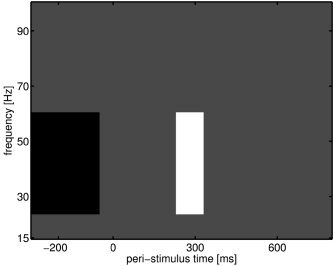
Contrast component for taking difference between two power averages, within trial. The gray values are zero, the black values are negative, and the white values are positive. The actual values are based on the total number of power values in each average.

For the parametric test, we derived a t‐statistic to test for a difference in power between conditions (P = 0.0498). For the nonparametric test (Wilcoxon), the P‐value was 0.0477. Both values are very close to each other and suggest further that the normal error assumption for this kind of data is appropriate. The difference from the P‐value originally reported by Tallon‐Baudry et al. [1998] is due to slightly different implementations of the processing scheme and lies in an expected range. Note that the lower P‐value of the nonparametric statistic does not contradict our finding that parametric statistics are, on average, more sensitive at a given false‐positive rate (Fig. 6). We also performed single subject analyses on all subjects to compare the parametric two‐sample t‐test to the Wilcoxon rank sum test (P‐values not reported). We found that subject‐wise parametric and nonparametric P‐values were very close to each other. Again, this suggests that parametric tests are appropriate for these data.

Applications

The key motivation for this work was to ensure the validity of parametric inference so that SPM could be used to analyze instantaneous power changes. SPM combines parametric inference with random field theory to provide P‐values adjusted for continuous search spaces. There are two useful applications to SPM. First, the analysis of (2D) time–frequency images, where the dimensions of the search space are time and frequency [Kilner et al., 2005]. These analyses pertain to a single channel or source. Second, as we will illustrate in a future communication, to apply SPM to baseline‐corrected power in source space. In this instance the search volume is over (3D) anatomical space.

CONCLUSION

We have shown how evoked and induced power, as measured with EEG/MEG, can be analyzed using parametric statistics. We found that the normal error assumption is appropriate for usual metrics of interest, i.e., the baseline‐corrected average over time and frequency. This assumption may be inappropriate for other metrics, e.g., instantaneous power. In these cases, we have shown that a nonlinear transform (log or sqrt) can be used to render the data normal. Normality allows one to make inferences using a standard parametric framework. We have established the validity and sensitivity of parametric tests using simulated and real EEG data.

The STFT and the MWT can be made equivalent, at a specific frequency, by choosing a Gaussian window for the STFT with the appropriate width. The equivalence of the BP/HT can be seen by noting that the convolution operator is linear, i.e., the Hilbert transform of bandpass‐filtered data h ^HT * h ^BP * y′ can also be described by (h ^HT * h ^BP) * y′. In other words, instead of applying the Hilbert transform to bandpass‐filtered data, one can also convolve the data with the Hilbert transformed bandpass filter kernel. This gives the analytic signal

(7)

The first kernel is the bandpass filter kernel h ^BP, and the second (complex) is its phase‐shifted version h ^HT * h ^BP. With a Gaussian window for the kernel h ^BP, one obtains equivalence among the three transforms. Clearly, this equivalence vanishes if one computes a time–frequency decomposition over more than one frequency. The STFT and BP/HT use, by default, the same window width at each frequency, whereas the MWT renders the width a function of frequency.

A further difference is that the window of the MWT is Gaussian, whereas the STFT and the bandpass filter can be applied with arbitrary forms. The bandpass filter does not need to conform to a windowed FIR filter [see, e.g., Tass et al., 2003]. In theory, free choice of the bandpass filter gives more latitude to the frequency response. However, with EEG/MEG the frequency response of interest is seldom defined sharply. For instance, between‐subject variability calls for averaging of power over frequencies. This averaging is likely to obscure any differences arising from the filter shape. If we assume that an FIR filter with a Gaussian window is sufficient to analyze induced oscillations, the key parameter, for all transforms, is the window width.

REFERENCES

- Barnes GR, Hillebrand A (2003): Statistical flattening of MEG beamformer images. Hum Brain Mapp 18: 1–12. [DOI] [PMC free article] [PubMed] [Google Scholar]
- Bracewell RN (1986): The Fourier transform and its applications, 2nd ed. Singapore: McGraw‐Hill. [Google Scholar]
- Breakspear M, Williams LM, Stam CJ (2004): A novel method for the topographic analysis of neural activity reveals formation and dissolution of ‘dynamic cell assemblies.’ J Computat Neurosci 16: 49–68. [DOI] [PubMed] [Google Scholar]
- Bruns A (2004): Fourier‐, Hilbert and wavelet‐based signal analysis: are they really different approaches? J Neurosci Methods 137: 321–332. [DOI] [PubMed] [Google Scholar]
- Durka PJ, Zygierewicz J, Klekowicz H, Ginter J, Blinowska K (2004): On the statistical significance of event‐related EEG desynchronization and synchronization in the time–frequency plane. IEEE Trans Biomed Eng 51: 1167–1175. [DOI] [PubMed] [Google Scholar]
- Henson RN, Goshen‐Gottstein Y, Ganel T, Otten LJ, Quayle A, Rugg MD (2003): Electrophysiological and haemodynamic correlates of face perception, recognition and priming. Cereb Cortex 13: 793–805. [DOI] [PubMed] [Google Scholar]
- Keil A, Stolarova M, Heim S, Gruber T, Muller MM (2003): Temporal stability of high‐frequency brain oscillations in the human EEG. Brain Topogr 16: 101–110. [DOI] [PubMed] [Google Scholar]
- Kiebel SJ, Friston KJ (2004): Statistical parametric mapping for event‐related potentials (II): a hierarchical temporal model. Neuroimage 22: 503–520. [DOI] [PubMed] [Google Scholar]
- Kilner J, Kiebel SJ, Friston KJ (2005): Applications of random field theory to electrophysiology. Neurosci Lett 374. [DOI] [PubMed] [Google Scholar]
- Le Van Quyen M, Foucher J, Lachaux J‐P, Rodriguez E, Lutz A, Martinerie J, Varela FJ (2001): Comparison of Hilbert transform and wavelet methods for the analysis of neuronal synchrony. J Neurosci Methods 111: 83–98. [DOI] [PubMed] [Google Scholar]
- Makeig S (1993): Auditory event‐related dynamics of the EEG spectrum and effects of exposure to tones. Electromyogr Clin Neurophysiol 86: 283–293. [DOI] [PubMed] [Google Scholar]
- Makeig S, Westerfield M, Jung T, Enghoff S, Townsend J, Courchesne E, Sejnowski T (2002): Dynamic brain sources of visual evoked responses. Science 295: 690–694. [DOI] [PubMed] [Google Scholar]
- Marple SL (1999): Computing the discrete‐time “analytic” signal via FFT. IEEE Trans Signal Process 47: 2600–2603. [Google Scholar]
- Marroquin JL, Harmony T, Rodriguez V, Valdes P (2004): Exploratory EEG data analysis for psychophysiological experiments. Neuroimage 21: 991–999. [DOI] [PubMed] [Google Scholar]
- Nuwer M (1988): Quantitative EEG. I. Techniques and problems of frequency analysis and topographic mapping. J Clin Neurophysiol 5: 1–43. [PubMed] [Google Scholar]
- Oppenheim A, Schafer R (1989): Discrete‐time signal processing. London: Prentice‐Hall International. [Google Scholar]
- Pfurtscheller G, Aranibar A (1977): Event‐related cortical desynchronization detected by power measurements of scalp EEG. Electroencephalogr Clin Neurophysiol 42: 817–826. [DOI] [PubMed] [Google Scholar]
- Tallon‐Baudry C, Bertrand O (1999): Oscillatory gamma activity in humans and its role in object representation. Trends Cogn Sci 3: 151–162. [DOI] [PubMed] [Google Scholar]
- Tallon‐Baudry C, Bertrand O, Delpuech C, Pernier J (1996): Stimulus specificity of phase‐locked and non‐phase‐locked 40 Hz visual responses in human. J Neurosci 16: 4240–4249. [DOI] [PMC free article] [PubMed] [Google Scholar]
- Tallon‐Baudry C, Bertrand O, Delpuech C, Pernier J (1997): Oscillatory γ‐band (30–70 Hz) activity induced by a visual search task in humans. J Neurosci 17: 722–734. [DOI] [PMC free article] [PubMed] [Google Scholar]
- Tallon‐Baudry C, Bertrand O, Peronnet F, Pernier J (1998): Induced γ‐band activity during the delay of a visual short‐term memory taks in humans. J Neurosci 18: 4244–4254. [DOI] [PMC free article] [PubMed] [Google Scholar]
- Tass P, Rosenblum M, Weule J, Kurths J, Pikovsky A, Volkmann J, Schnitzler A, Freund H‐J (1998): Detection of n:m phase locking from noisy data: application to magnetoencephalography. Phys Rev Lett 81: 3291–3294. [Google Scholar]
- Tass P, Fieseler T, Dammers J, Dolan K, Morosan P, Majtanik M, Boers F, Muren A, Zilles K, Fink G (2003): Synchronization tomography: a method for three‐dimensional localization of phase synchronized neuronal populations in the human brain using magnetoencephalography. Phys Rev Lett 90: 88–101. [DOI] [PubMed] [Google Scholar]