Variability in fMRI: A re‐examination of inter‐session differences

INTRODUCTION

The blood oxygenation level‐dependent (BOLD) effect in functional magnetic resonance imaging (fMRI), a marker of neuronal activation, is often only of similar magnitude to the noise present in the measured signal. To increase power and to allow conclusions to be made about subject populations, it is common practice to combine data from multiple subjects. It is also common to take multiple sessions from each subject, again to increase sensitivity to activation, or for other experimental design reasons such as tracking changes in function over time. It is therefore important that inter‐session variability present in fMRI data is understood, and in response, McGonigle et al. [2000] presented an in‐depth study of this issue.

In designing both multi‐subject and single‐subject multisession studies, it is critical for the experimenter to have some idea of the relative sizes of within‐session variance and inter‐session variance. For example, if inter‐session variance is large, it could be difficult to detect longitudinal experimental effects (e.g., in studies of learning [Ungerleider et al., 2002] and poststroke recovery [Johansen‐Berg et al., 2002]). If fMRI is to be used in presurgical mapping [e.g., Fernandez et al., 2003], which by its nature will involve only a single subject, correct interpretation will be dependent on an appreciation of the potential uncertainty due simply to a session effect. In multi‐subject studies, it is advantageous to have some idea of the expected inter‐session variance, as this will contribute to the observed inter‐subject variance.

To investigate how well a single‐session dataset from a single subject typified the subject's responses across multiple sessions, McGonigle et al. [2000] carried out the same fMRI protocol on 33 separate days. On each day, three paradigms were run (visual, motor, and cognitive), and the variation in activation was studied. The study drew three main conclusions: (1) the use of voxel‐counting on thresholded statistical maps was not an ideal way to examine reproducibility in fMRI; (2) a reasonably large number of repeated sessions was essential to properly estimate inter‐session variability; and (3) the results of a single session from a single subject should be treated with care if nothing was known about inter‐session variability.

Although McGonigle et al. [2000] noted the presence of between‐session variability in their experiment, they did not attempt to assess systematically the causes of this variance. There are a number of potential contributors, such as physiologic variance (subject), acquisition variance (scanner), and differences in analysis methodology and implementation. As noted in their original article, “it is possible that spatial preprocessing (for example) may affect inter‐session variance quite independently of underlying physical or physiological variability.” This view is supported by Shaw et al. [2003], where analysis methodology is shown to affect apparent inter‐session variance. In the present study, we revisit the analysis of data from McGonigle et al. [2000] and consider session variability in the light of the effects that different first‐level processing methods can have.

Others have taken from McGonigle et al. [2000] the simple broadbrush conclusion that there was a “large amount of session variability” [e.g., Beisteiner et al., 2001; Chee et al., 2003]. One of the purposes here is to address this misconception; for example, we show that for this dataset, inter‐session variability was of similar magnitude to within‐session variability.

We start with a brief theoretical overview of the components of variance present in multiple‐session data. We then describe the original data and analysis, as well as the new analyses carried out for this study, with explanation of the measures used in this study to assess session variability. We then present the variability results as found from these data, centering around the use of mixed‐effects Z values in relevant voxels as the primary measure of interest. We also show qualitatively why it is dangerous to judge variability through the use of thresholded single‐session images.

Variance Components

Researchers often refer to different group analyses, the most common being fixed‐effects and mixed‐effects. What these terms are actually referring to are different inter‐session (or inter‐subject) noise (variance) models. We now summarize what the terms and associated models mean.

We start with the equation for the t‐statistic:

(1)

i.e., we are asking how big the mean effect size is compared to the noise (the mean's standard deviation1). The standard deviation is the square root of either the fixed‐effects variance of the mean or the random‐effects variance of the mean.

With fixed‐effects modeling, we assume that we are only interested in the factors and levels present in the study, and therefore our higher‐level fixed‐effects variance FV is derived from pooling2 the first‐level (within‐session) variances (of first‐level effect size mean) FV _i, according to:

(2)

where DoF is the degrees of freedom, which is usually large in the case of fMRI time series. This modeling therefore ignores the cross‐session (or cross‐subject) variance completely and the results cannot be generalized outside of the group of sessions/subjects involved in the study.

With simple mixed‐effects3 modeling, we derive the mixed‐effects variance MV directly from the variance of the first‐level parameter estimates PE _i (effect sizes) or contrasts of parameter estimates:

(3)

with a (normally) much smaller DoF than with fixed‐effects. The modeling thus uses the cross‐session (or cross‐subject) variance, and the results (which are generally more conservative than with a fixed‐effects analysis) are relevant to the whole population from which the group of sessions/subjects was taken.

The mixed‐effects variance is the sum of the fixed‐effects (within‐session) variance and random‐effects (pure inter‐session) variance, although simple estimation methods calculate this directly, as above, and do not explicitly use the fixed‐effects variance. The estimated mixed‐effects variance therefore should in theory and in practice be larger than the fixed‐effects variance. We expect that when there is large inter‐session variance, there will be a large difference between fixed‐ and mixed‐effects analyses.

There have been recent significant developments in group‐level analysis. For example, it has been shown [Beckmann et al., 2003a] that there is value in carrying up lower‐level variances to higher‐level analyses of mixed‐effects variance, and one implementation of this using Bayesian modeling/estimation methodology has been reported [Woolrich et al., 2003]. Whereas the dataset used in this study may well prove useful in investigating these developments further, this is beyond the scope of this article. Instead, we concentrate primarily on two other questions, namely the magnitude of session variability, and the effect that first‐level analysis methodologies can have on its apparent magnitude. For mixed‐effects analyses in the present work, we therefore have only used ordinary least‐squares (OLS) estimators (see equation [3] and [Holmes and Friston, 1998]).

MATERIAL AND METHODS

Original Experiments and Analysis

We describe here the experiment and original analysis carried out by McGonigle et al. [2000]. A healthy, 23‐year‐old, right‐handed male was scanned on 33 separate days (over 2 months) with as many factors as possible held constant. On each day, three block‐design paradigms were run (all using block lengths for rest = 24.6 s and activation = 24.6 s): visual (8‐Hz reversing black‐white checkerboard, 36 time points after deleting the first two); motor (finger tapping, right index finger at 1.5 Hz, 78 time points); and cognitive (0.66‐Hz random number generating vs. counting, 78 time points), with the paradigm order randomized. The data were collected on a Siemens Vision at 2 T (repetition time [TR] = 4.1 s, 64 × 64 × 48, 3 × 3 × 3 mm voxels). A single T1‐weighted 1.5 × 1 × 1 mm structural scan was taken.

Original analysis was carried out using SPM99 (online at http://www.fil.ion.ucl.ac.uk/spm). All 99 sessions were realigned (motion‐corrected) to the same target (the first scan of the first session of the first day) and then a mean over all 99 sessions was created. This was used to find normalization (to a T2‐weighted target in MNI space [Evans et al., 1993]) parameters for all 99 sessions (using 12‐parameter affine followed by 7 × 8 × 7 basis‐function nonlinear registration). Sinc interpolation on final output was used.

Sessions containing “obvious movement artefacts” were identified by eye and removed from consideration (three motor, two visual, and three cognitive). Cross‐session analysis was carried out for voxels in standard space that were present in all sessions. Spatial filtering with a Gaussian kernel of full‐width half‐maximum (FWHM) 6 mm was applied. Each volume of each session was intensity normalized (rescaled) so that all had the same mean intensity.

Voxel time‐series analysis was carried out using general linear modeling (GLM). The data was first precolored by temporally smoothing the data with a Gaussian of 6 s FWHM. Slow drifts in the data were removed by including drift terms in the model (a set of cosine basis functions effectively removing signals of period longer than 96 s).

For presentation of within‐session results, voxel‐wise thresholding (P < 0.05) was used, correcting for multiple comparisons using Gaussian random field theory (GRF) [Friston et al., 1994].

Both fixed‐ and mixed‐effects analyses were carried out to examine the effects of using different variance components, and an extra‐sum‐of‐squares (ESS) F‐test was performed across all sessions of each paradigm to assess the presence of significant inter‐session variance.

Methods Tested

We now describe the analysis approaches used for this article. The two packages used for our investigations were SPM99b (Statistical Parametric Mapping) and FSL v1.3 (FMRIB Software Library; online at http://www.fmrib.ox.ac.uk/fsl, June 2001). Both are available freely and used widely.

SPM includes a motion‐correction (realignment) tool, a tool for registration (normalization) to standard space, GLM‐based time‐series statistics [Worsley and Friston, 1995], and GRF‐based inference [Friston et al., 1994]. SPM carries out standard‐space registration before time‐series statistics. The SPM99b time series statistics correct for temporal smoothness by precoloring [Friston et al., 2000].

GLM‐based analysis in FSL is carried out with the fMRI Expert Analysis Tool (FEAT), which uses other FSL tools such as Brain Extraction Tool (BET [Smith, 2002]), an affine registration tool, FMRIB's Linear Image Registration Tool (FLIRT [Jenkinson and Smith, 2001; Jenkinson et al., 2002]), and a motion‐correction tool based on FLIRT (MCFLIRT [Jenkinson et al., 2002]). FEAT carries out standard‐space registration after time‐series statistics. FSL time‐series statistics correct for temporal smoothness by applying prewhitening [Woolrich et al., 2001].

Six different, complete analyses were carried out with various combinations of preprocessing and time‐series statistics options to allow a variety of comparisons to be made. In tests A, C, and G, FSL was used for preprocessing and registration whereas in tests D, E, and F, SPM was used. For tests A, D, and G, FEAT time‐series statistics was used whereas for C, E, and F, SPM time‐series statistics was used.

In tests A–E, the various controlling parameters were kept as similar as possible, both to each other and to default settings in the relevant software packages. Tests A versus D and C versus E hold the statistics method constant while comparing spatial methods, therefore showing the relative merits of the spatial components (motion correction and registration). Tests A versus C and D versus E hold the spatial method constant while comparing statistical components, thus showing the relative merits of the statistical components (time‐series analysis). A versus E tests pure‐FSL against pure‐SPM. F and G test pure‐SPM and pure‐FSL, respectively, with these analyses set up to match the specifications of the original analyses in McGonigle et al. [2000] as closely as possible, including turning on intensity normalization in both cases. For a summary, see Table I. (For B, model‐free independent component analysis (ICA) was carried out; the model‐free results are not included here but will be presented elsewhere.)

Table I.

Different analyses carried out

Test	Preprocessing	Statistics	Registration
A	FSL (MCFLIRT spat = 5 intnorm = n)	FSL (FEAT) (hp‐FSL = 40)	FSL (FLIRT)
C	FSL (MCFLIRT spat = 5 intnorm = n)	SPM (hp‐cos = 72)	FSL (FLIRT)
D	SPM (SPM‐mc&norm spat = 5 intnorm = n)	FSL (FEAT) (hp‐FSL = 40)	SPM (done in preproc)
E	SPM (SPM‐mc&norm spat = 5 intnorm = n)	SPM (hp‐cos = 72)	SPM (done in preproc)
F	SPM match [18] (SPM‐mc&norm spat = 6 intnorm = y)	SPM (hp‐cos = 98.4)	SPM (done in preproc)
G	FSL match [18] (MCFLIRT spat = 6 intnorm = y)	FSL (FEAT) (hp‐FSL = 53)	FSL (FLIRT)

Spat, spatial filtering with full‐width‐half‐maximum given in mm.

intnorm, intensity normalization (the intensity rescaling of each volume in a 4‐D fMRI dataset so that all have the same mean within‐brain intensity).

hp‐FSL, FSL's high‐pass temporal filtering with cutoff period given in seconds.

hp‐cos, high‐pass temporal filtering (in seconds) via cosine basis functions.

preproc, preprocessing.

Because the methods for high‐pass temporal filtering in FSL and SPM are intrinsically different, they cannot be set to act in exactly the same way (within A–E and within F and G) by choosing the same cutoff period in each; instead, the cutoff choices were made to match as closely as possible the extent to which the relevant signal and noise frequencies were attenuated by the different methods. For the purposes of the present work, high‐pass temporal filtering is considered part of the temporal statistics, where it fits most naturally. The non‐default “Adjust for sampling errors” motion‐correction option in SPM was not used.

Eight sessions (of the 99) were excluded from the original analysis in McGonigle et al. [2000] due to “obvious movement artefacts.” These were included in our analyses, however, as we did not consider that there was sufficient objective reason to exclude them. The estimated motions for these sessions were not, in general, significant outliers relative to the average motion across sessions and any apparent (activation map) motion artefacts were not in general significantly different from most of the sessions. The quantitative results below were in fact recalculated without these eight sessions, i.e., reproducing the same dataset as used in McGonigle et al. [2000], but without any significant change in results, and therefore are not reported here.

Inter‐Session Evaluation Methods

For all paradigms and analysis methods, simple fixed‐effects (FE) and OLS mixed‐effects (ME) Z‐statistics were formed. For each paradigm, a mask of voxels that FE considered potentially activated (Z > 2.3) was created. This contains voxels in which an ME analysis is potentially interested (given that ME generally gives lower Z‐statistics than does FE4). This mask was averaged over A, C, D, and E to balance across the various methods, and then eroded slightly (2 mm in 3D) to avoid possible problems due to different brain mask effects.

We initially investigated the size of inter‐session variance by estimating the ratio of random‐effects variance to fixed effects, averaged over the voxels of interest as defined above. Given that ME variance is the sum of FE and RE variance, we estimated the RE (inter‐session) variance by subtracting the FE variance from the ME variance. We then took the ratio image of RE to FE variance, and averaged over the masks described above. This ratio would be 0 if there were no inter‐session variability and rises as the contribution by inter‐session variability increases. A ratio of 1 occurs when inter‐ and intra‐session variabilities make similar contributions to the overall measured ME variance.

We next investigated whether session variability is indeed Gaussian distributed. If it is not, then inference based on the OLS method used for ME modeling and estimation in the present work would need a much more complicated interpretation (as also would be the case with many other group‐level methods used in the field). We used the Lilliefors modification of the Kolmogorov‐Smirnov test [Lilliefors, 1967] to measure in what fraction of voxels the session effect was significantly non‐Gaussian.

The variance ratio figures do not take into account estimated effect size, which in general will vary between methods, and so the primary quantification in this study uses the mixed‐effects Z (ME‐Z). This is roughly proportional to the mean effect size and inversely proportional to the inter‐session variability. This makes ME‐Z a good measure with which to evaluate session variability; it is affected directly by the variability while being weighted higher for voxels of greater interest (i.e., voxels containing activation). We are not particularly interested in variability in voxels that contain no mean effect. We therefore base our cross‐subject quantitation on ME‐Z comparisons within regions of interest (defined above).5

If one of the analysis methods tested here results in increased ME‐Z, then this implies reduced overall method‐related error (increased accuracy) in the method, because unrelated variances add. Although a single‐session analysis cannot eliminate true inter‐session variance intrinsic to the data, it can add (induce) variance to the effective inter‐session variance due to failings in the method itself (for example, poor estimates of first‐level effect/variance, or registration inaccuracies). The best methods should therefore give ME‐variance that approaches (from above) the true, intrinsic inter‐session ME‐variance. Recall that the same simple OLS second‐level estimation method was used for all analyses carried out, and it is only the first‐level processing that is varied.

Mean ME‐Z was then calculated within the FE‐derived masks. As well as reporting these uncorrected mean ME‐Z values, we also report the mean values after adjusting the ME‐Z images for the fact that in their histograms (supposedly a combination of a null and an activation distribution) the null part, ideally a zero mean and unit standard deviation Gaussian, was often significantly shifted away from having the null peak at zero. This makes Z‐values incomparable across methods, and needed to be corrected for. The causes of this effect include spatially structured noise in the data and in differences in the success between the different methods for correcting for temporal smoothness, a problem enhanced potentially for all methods given the unusually low number of time points in the paradigms.

We used two methods to correct ME‐Z for null‐distribution imperfections, and report results for both methods. With hand‐corrected peak shift correction, the peak of the ME‐Z distribution was identified by eye and assumed to be the mean of the null distribution; the ME‐Z image then had this value subtracted. With mixture‐model‐based null shift correction, a nonspatial histogram mixture model was automatically fitted to the data using expectation‐maximization. This involved a Gaussian for the null part, and gammas for the activation and deactivation parts [Beckmann et al., 2003b]. The center of the Gaussian fit was then used to correct the ME‐Z image. The advantage of the hand‐corrected method is that it is potentially less sensitive to failings in the assumed form of the mixture components; the advantage of the mixture‐model‐corrected fit is that it is fully automated and therefore more objective.

It is not yet standard practice (with either SPM or FSL) to correct for null‐Z shifts in ME‐Z histograms; the most common method of inference is to use simple null hypothesis testing on uncorrected T or Z maps (typically via Gaussian random field theory). By correcting for the shifts, we are able to investigate the effects of using the different individual analysis components in the absence of confounding effects of null distribution imperfections.

Figure 1 shows an example ME‐Z histogram including the estimates (by eye and mixture‐modeling) of the null mode. The estimated ME‐Z shifts that were applied to the mean ME‐Z values before comparing methods are plotted for all analysis methods and all paradigms in Figure 2. The shift is clearly more related to the choice of time‐series statistics method than to the choice of spatial processing method (motion correction and registration), but there is no clear indication of one statistics method giving a greater shift extent than another. The two correction methods are largely in agreement with each other.

Figure 1.

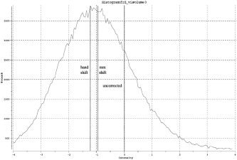
Example ME‐Z histogram showing null‐distribution shift, from analysis A of the visual paradigm.

Figure 2.

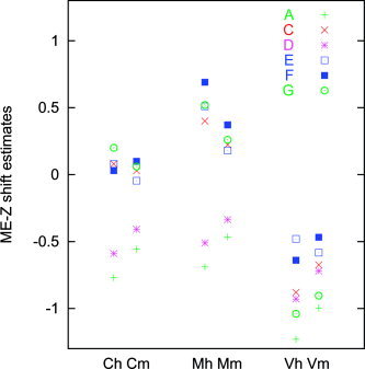
Estimated ME‐Z null distribution shifts. Different tasks: C, cognitive; M, motor; V, visual. Different correction methods: h, hand‐shifted; m, mixture‐model‐shifted.

RESULTS AND DISCUSSION

Fixed‐Effects Activation Maps

The FE‐based mask images (used to define the voxels used in the quantitative analyses reported below) are shown in Figure 3 as overlaid onto the MNI152 standard head image.

Figure 3.

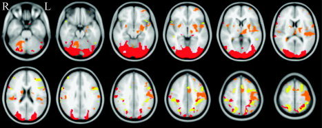
Masks of potentially activated voxels, within which mean ME‐Z was calculated for each analysis method. Red, visual; orange, motor; yellow, cognitive.

Inter‐Session Effect Size Plots

For analysis methods A and E, we now show the effect size and its (fixed‐effects, within‐session) temporal standard deviation, as a function of session number. Both the effect size and the temporal standard deviation are estimated as means over interesting voxels, as defined above. The plots were normalized by estimating the mean effect size over all sessions, scaling this to be unity, scaling the standard deviation by the same factor, and demeaning the effect size plot (Figs. 4 and 5). These plots show (as does the following section) that the within‐session variance has similar magnitude to the inter‐session variance. They also show that variability in effect size is higher than variability in its standard deviation (although the implication of this fact is not necessarily important to the primary points in the present work). The results presented here correspond to the uncorrected plot in Figure 8.

Figure 4.

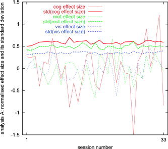
Mean first‐level effect size and its (within‐session) standard deviation, as a function of session number, for analysis A.

Figure 5.

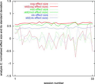
Mean first‐level effect size and its (within‐session) standard deviation, as a function of session number, for analysis E.

Figure 8.

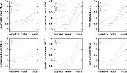
Mean mixed‐effects Z‐values, uncorrected and with both Z‐shift correction methods.

Quantification of Inter‐Session Variance

To quantitate better the size of inter‐session variance, we estimated the mean ratio of RE (ME minus FE) to FE variance. Any comparison between the RE and FE variance will be dependent on the number of time points in each session, with a larger number of time points leading to an increase in the RE:FE ratio.

The results are shown in Table II. The interpretation of this is simple yet important: in these datasets, inter‐session variability is not large compared to within‐session variability.6

Table II.

Mean estimated ratio of RE (inter‐session) variance to FE (within‐session pooled) variance

Paradigm	Test
	A	C	D	E	F	G
Cognitive	1.0	0.3	1.5	0.5	0.6	1.0
Motor	0.9	0.3	1.4	0.6	0.6	1.1
Visual	1.4	0.3	1.9	0.8	0.8	1.7

We cannot make very useful interpretations of the variations across methods of the variance ratio, particularly without also taking into account the estimated effect size; hence the use of mixed‐effects Z for the main method comparison results shown below.

Test for Gaussianity of Inter‐Session Variability

Using the results of analysis A, for each paradigm we tested whether the session variability was Gaussian. At each voxel in standard space, we took the (first‐level) parameter estimates (effect sizes) from the relevant voxel in each of the 33 relevant first‐level analyses, (i.e., the same data that was fed into the group‐level ME analysis). The variance of these is the ME variance. For each set of 33 first‐level parameter estimates, we ran the Lilliefors modification of the Kolmogorov‐Smirnov test [Lilliefors, 1967] for non‐Gaussianity, with a significance threshold of 0.05. In null data, we would therefore expect rejection of the Gaussianity null hypothesis at this 5% rate by random chance.

We calculated the fraction of voxels failing the normality test across the whole brain and within the FE‐derived masks described above. In both cases and for all three paradigms, the fraction of failed tests was less than 7.5% (range, 4.5–7.3%), which is very close to the expected 5% rate of null hypothesis rejections if in fact all the data is normal. This provides strong quantitative evidence for the normality of the session variability in this data. Qualitatively, the voxels where the null hypothesis was rejected were scattered randomly through the images, not clumped, again suggesting that they were rejected by pure random chance rather than because of some true underlying non‐Gaussian process.

On (Not) Drawing Conclusions About Session Variability Based on Thresholded Single‐Session Images

McGonigle et al. [2000] does not include any such statement as “session variability is high,” or even any quantification explicitly suggesting in a simple way that session variability is a serious problem. Nevertheless, unfortunately, many researchers [e.g., Beisteiner et al., 2001; Chee et al., 2003] seem to have taken these messages from the study. One of the causes of this is the apparent variability in Figures 2, 3, 4 in McGonigle et al. [2000], which show for each paradigm each session's thresholded activation image (as a single sagittal slice maximum intensity projection). All three figures give the impression of large inter‐session variability, even for the strong visual paradigm.

The most important point to make with respect to this issue is that it is not safe to judge inter‐session variability by looking at variability in thresholded statistic images. It is perfectly possible for two unthresholded activation images to not be significantly different statistically and yet one contains activation just over threshold and the other just under, giving the false impression of large variability. The fact that thresholds are in any case chosen arbitrarily increases the weakness of this method of judging variability.

To illustrate these issues, Figures 6 and 7 show single‐session thresholded images from analysis F of the visual experiment. Figure 6 is created using the same threshold as that used in McGonigle et al. [2000], namely P < 0.05, corrected for multiple comparisons using Gaussian random field theory [Friston et al., 1994]. In contrast, Figure 7 is created using a reduced threshold (the t threshold used in Figure 6 is reduced by 33%). Obviously there is more apparent activation when the threshold is reduced (although it has clearly not been reduced so far that there is generally a huge amount of spatially variable noise activation caused by this). The interesting point, however, is that the subjective impression of inter‐session variability is much reduced.

Figure 6.

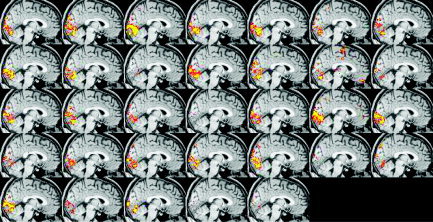
Visual paradigm; analysis F single‐session thresholded maximum intensity projections, P < 0.05 GRF‐corrected. Each image corresponds to a different day's dataset.

Figure 7.

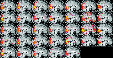
Visual paradigm; analysis F single‐session thresholded maximum intensity projections, thresholded with the t threshold reduced from the “P < 0.05 GRF‐corrected” level by 33%. Note that as well as the obvious increase in reported activation, “apparent variability” is decreased significantly.

Finally, a question arises as to why Figure 6, which should match the original figure in McGonigle et al. [2000] having been processed in the same manner, seems to show less variability than that in the original figures. This was found to be because suboptimal timing was used in the original model generation (caused by a particular default setting of the point within a TR that the model is sampled, which also corresponds to the point during a TR when that time point's whole fMRI volume is assumed to have been sampled instantaneously; this default was changed between SPM99 and SPM99b). The reanalysis was more efficient at estimating activation as better‐matched models were used, causing less apparent inter‐session variability.

As part of the investigation of this effect, we tested the variability in peak Z‐values as the model timing was changed slightly. The mean‐across‐sessions (max‐across‐space[Z]) value for five different phase shifts of the model (−1 TR to +1 TR) were found to be 6.6, 7.5, 7.9, 7.5, 6.9 (model timing running from earlier to later, respectively). This is quite a large effect for these phase shifts, given that the paradigm is a block design. This is another illustration of the danger of judging variability solely based on thresholded results.

Mean ME‐Z Plots

Mean ME‐Z plots are shown in Figure 8. Higher ME‐Z implies less analysis‐induced inter‐session variance, or viewed another way, greater robustness to session effects.

Before discussing these plots it is instructive to get a feeling for what constitutes significant difference in the plots. Suppose that in these figures, two ME‐Z maps were separated by a Z difference of 0.25. This would correspond to a general relative scaling between the two maps of approximately 0.25/6 = 4%. We are interested in the effect that this difference has on the final thresholded activation map. We can therefore estimate this effect by thresholding an ME‐Z map at a standard level and at this level scaled by 4%. Thresholding at P < 0.05, when corrected (using Gaussian random field theory) for multiple comparisons, corresponds to a Z threshold of approximately 5. We therefore thresholded the three ME‐Z images from analysis F at levels of Z > 5 and Z > 5.2. For the cognitive, motor, and visual ME‐Z images, this resulted in reductions in suprathreshold voxel counts by 11, 8, and 6%, respectively. These are not small percentages; we conclude that a difference in 0.25 between the various plots can be considered significant in terms of the effect on the final reported mixed‐effects activation maps. Note that these different thresholdings were carried out with two threshold levels on the same ME‐Z image for each comparison, hence the previous criticism of not comparing thresholded maps is not relevant here.

We consider here plots A, C, D, and E, the various tests that attempted to match all settings both to each other and to default usage. Firstly, consider comparisons that show the relative merits of the spatial components (motion correction and registration): A versus D and C versus E hold the statistics method constant while comparing spatial methods. Next, consider comparisons that show the relative merits of the statistical components (time‐series analysis): A versus C and D versus E hold the spatial method constant while comparing statistical components. Finally, A versus E tests pure‐FSL against pure‐SPM.

Plots F and G test pure‐SPM and pure‐FSL, respectively, with these analyses set up to match the specifications of the original analyses in McGonigle et al. [2000], including turning on intensity normalization in both cases.

The results show that both time‐series statistics and spatial components (primarily head motion correction and registration to standard space) add to apparent session variability. Overall, with respect both to spatial alignment processing and time‐series statistics, FSL induced less error than did SPM, i.e., was more efficient with respect to higher‐level activation estimation.

The experiments used a block‐design, and as such are not expected to show up the increased estimation efficiency of prewhitening over precoloring [Woolrich et al., 2001]. In a study similar to that presented here [Bianciardi et al., 2003], first‐level statistics were obtained using SPM99 and FSL (i.e., only time‐series statistics were compared, not different alignment methods). The data were primarily event related and, as in this work, simple second‐level mixed‐effects analysis was used to compare efficiency of the different methods. The results showed that prewhitening was not just more efficient at first‐level, but also gave rise to increased efficiency in the second‐level analysis.

Intensity Normalization

FEAT offers the option of intensity normalization of all volumes in each time series to give constant mean volume intensity over time; however, this option is turned off by default, as it is considered that this is an oversimplistic approach to a complicated problem [see for example De Luca et al., 2002].

We investigated the effect on inter‐session variance of turning intensity normalization on. It was found that this preprocessing step does reduce the overall fixed‐ and random‐effects variance (on average by about 10%), and therefore slightly increases the fixed‐ and random‐effects Z‐values (again giving on average approximately a 10% increase in the number of suprathreshold voxels).

One‐ or Two‐Step Registration

FEAT does not transform the fMRI data directly into standard space but carries all statistics out in the original (low‐resolution) space and then transforms the final statistics images into standard space. The transformation from original space into standard space is carried out normally (automatically) in a two‐step process. First, an example functional image (the one used as the reference in the motion correction) is registered to the subject's structural image (normally a T1‐weighted image that has been brain‐extracted using BET [Smith, 2002]) and then the structural image is registered to a standard space template (normally the MNI152). The two resulting transformations are concatenated resulting in a single transform that takes the low‐resolution statistic images into standard space. This is the default FEAT registration procedure and is what was used for the analyses presented above.

We investigated whether for this data FEAT's two‐step process (using FLIRT) is an improvement over registering the example functional image directly into standard space (using FLIRT). The two‐step registration resulted in a slight decrease in cross‐session fixed‐ and random‐effects overall variance (by approximately 3%). The number of activated voxels in general stayed the same, but the peak Z‐statistic improved (again by approximately 3%) when two‐step registration was used and the activation seemed qualitatively to contain more structural detail (i.e., was less blurred). The conclusion therefore is that even for this within‐subject across‐session analysis, the two‐step registration approach was of value in the FEAT analyses.

CONCLUSIONS

Inter‐session variability is an important consideration in power calculations for the design of fMRI experiments. It is also a critical issue for interpretation of studies that allow for only single observations, e.g., in many clinical applications of fMRI. We have provided here quantitative data confirming that inter‐session variability in fMRI is not large relative to within‐session variability. We also emphasize that inter‐session variability should not be judged by apparent variability in thresholded activation maps.

There are several mechanisms by which inter‐session variability can be minimized. Although considerable attention has been paid in the past to hardware and experimental design factors, we have shown here that additional benefits can come with optimization of analysis methodology, as analysis methods add extra variance to the true inter‐session variance, causing an apparent increase in inter‐session variance. It was found that with respect both to spatial alignment processing and time‐series statistics, FSL v1.3 induced less error than did SPM99b, i.e., was more efficient with respect to higher‐level activation estimation.

REFERENCES

- Beckmann CF, Jenkinson M, Smith SM (2003a): General multilevel linear modeling for group analysis in fMRI. Neuroimage 20: 1052–1063. [DOI] [PubMed] [Google Scholar]
- Beckmann CF, Woolrich MW, Smith SM (2003b): Gaussian/gamma mixture modelling of ICA/GLM spatial maps. Neuroimage 19(Suppl): 985. [Google Scholar]
- Beisteiner R, Windischberger C, Lanzenberger R, Edward V, Cunnington R, Erdler M, Gartus A, Streibl B, Moser E, Deecke L (2001): Finger somatotopy in human motor cortex. Neuroimage 13: 1016–1026. [DOI] [PubMed] [Google Scholar]
- Bianciardi M, Cerasa A, Hagberg G (2003): How experimental design and first‐level filtering influence efficiency in second‐level analysis of event‐related fMRI data. Neuroimage 19(Suppl): 785. [Google Scholar]
- Chee MW, Lee HL, Soon CS, Westphal C, Venkatraman V (2003): Reproducibility of the word frequency effect: comparison of signal change and voxel counting. Neuroimage 18: 468–482. [DOI] [PubMed] [Google Scholar]
- De Luca M, Beckmann CF, Behrens T, Clare S, Matthews PM, De Stefano N, Woolrich M, Smith SM (2002): Low frequency signals in FMRI—“resting state networks” and the “intensity normalisation problem.” In: Proc Int Soc Magn Reson Med, 10th Annual meeting, Honolulu, USA.
- Evans AC, Collins DL, Mills SR, Brown ED, Kelly RL, Peters TM (1993): 3D statistical neuroanatomical models from 305 MRI volumes. In: Proc IEEE‐Nuclear Science Symposium and Medical Imaging Conference. p 1813–1817.
- Fernandez G, Specht K, Weis S, Tendolkar I, Reuber M, Fell J, Klaver P, Ruhlmann J, Reul J, Elger CE (2003): Intrasubject reproducibility of presurgical language lateralization and mapping using fMRI. Neurology 60: 969–975. [DOI] [PubMed] [Google Scholar]
- Friston KJ, Josephs O, Zarahn E, Holmes AP, Rouquette S, Poline JB (2000): To smooth or not to smooth? Neuroimage 12: 196–208. [DOI] [PubMed] [Google Scholar]
- Friston KJ, Worsley KJ, Frackowiak RSJ, Mazziotta JC, Evans AC (1994): Assessing the significance of focal activations using their spatial extent. Hum Brain Mapp 1: 214–220. [DOI] [PubMed] [Google Scholar]
- Holmes AP, Friston KJ (1998): Generalisability, random effects and population inference. Neuroimage 7(Suppl): 754. [Google Scholar]
- Jenkinson M, Bannister PR, Brady JM, Smith SM (2002): Improved optimisation for the robust and accurate linear registration and motion correction of brain images. Neuroimage 17: 825–841. [DOI] [PubMed] [Google Scholar]
- Jenkinson M, Smith SM (2001): A global optimisation method for robust affine registration of brain images. Med Image Anal 5: 143–156. [DOI] [PubMed] [Google Scholar]
- Johansen‐Berg H, Dawes H, Guy C, Smith SM, Wade DT, Matthews PM (2002): Correlation between motor improvements and altered fMRI activity after rehabilitative therapy. Brain 125: 2731–2742. [DOI] [PubMed] [Google Scholar]
- Leibovici DG, Smith S (2000): Comparing groups of subjects in fMRI studies: a review of the GLM approach. Technical Report TR00DL1, Oxford Centre for Functional Magnetic Resonance Imaging of the Brain, Department of Clinical Neurology, Oxford University, Oxford, UK. Available at http://www.fmrib.ox.ac.uk/analysis/techrep for downloading.
- Lilliefors L (1967): On the Kolmogorov‐Smirnov test for normality with mean and variance unknown. J Am Stat Assoc 62: 399–402. [Google Scholar]
- McGonigle DJ, Howseman AM, Athwal BS, Friston KJ, Frackowiak RSJ, Holmes AP (2000): Variability in fMRI: an examination of intersession differences. Neuroimage 11: 708–734. [DOI] [PubMed] [Google Scholar]
- Shaw ME, Strother SC, Gavrilescu M, Podzebenko K, Waites A, Watson J, Anderson J, Jackson G, Egan G (2003): Evaluating subject specific preprocessing choices in multisubject fMRI data sets using data‐driven performance metrics. Neuroimage 19: 988–1001. [DOI] [PubMed] [Google Scholar]
- Smith SM (2002): Fast robust automated brain extraction. Hum Brain Mapp 17: 143–155. [DOI] [PMC free article] [PubMed] [Google Scholar]
- Ungerleider LG, Doyon J, Karni A (2002): Imaging brain plasticity during motor skill learning. Neurobiol Learn Mem 78: 553–564. [DOI] [PubMed] [Google Scholar]
- Woolrich MW, Behrens TEJ, Beckman CF, Jenkinson M, Smith SM (2004): Multi‐level linear modelling for fMRI group analysis using Bayesian inference. Neuroimage 21: 1732–1747. [DOI] [PubMed] [Google Scholar]
- Woolrich MW, Ripley BD, Brady JM, Smith SM (2001): Temporal autocorrelation in univariate linear modelling of FMRI data. Neuroimage 14: 1370–1386. [DOI] [PubMed] [Google Scholar]
- Worsley KJ, Friston KJ (1995): Analysis of fMRI time series revisited—again. Neuroimage 2: 173–181. [DOI] [PubMed] [Google Scholar]