

Abstract
In this article we describe a new method, using SPM99, that searches explicitly for bilateral structural abnormalities. Children with bilateral pathology have a poorer prognosis than children with unilateral damage. After brain injury or disease in childhood, it is thought that rescue of function is only possible if the neuronal substrates of that function are preserved and operational in at least one hemisphere [Vargha‐Khadem and Mishkin, 1997]. If this is the case, the detection of bilateral abnormalities would greatly facilitate more accurate prognosis in children with brain injury or developmental disorders. We have therefore developed a technique to detect bilateral abnormalities that uses conjunction analysis with voxel based morphometry. It is illustrated using a group of patients with bilateral hypoxic‐ischaemic damage to the hippocampus. The approach is shown to have enhanced specificity and sensitivity relative to conventional unilateral characterisations. Hum. Brain Mapping 11:223–232, 2000. © 2000 Wiley‐Liss, Inc.
Keywords: voxel‐based morphometry, bilateral abnormalities, conjunctions
INTRODUCTION
In this article we describe a technique that detects bilateral structural abnormalities using voxel‐based morphometry and new results from Gaussian Random Field theory that enable inferences about conjoint changes in homologous brain regions. We first review voxel‐based morphometry (VBM), discuss the importance of bilateral changes, and introduce VBM for bilateral effects using conjunction analyses.
Voxel‐based morphometry
Voxel‐based morphometry was developed to characterise cerebral grey and white matter differences in structural MRI scans. In contrast to other methods, which frame the search in terms of regions of interest, voxel‐based morphometry detects structural differences with uniform sensitivity throughout the brain. Voxel‐based morphometry is essentially a technique that compares images of grey matter (obtained from segmented MRI images). This comparison uses statistical parametric mapping to identify, and make inferences about, regionally specific differences.
Voxel‐based morphometry has been used to look at structural abnormalities in a variety of patient populations. Wright et al. [1995] first used it to examine schizophrenic patients. They found correlations between syndrome scores and grey and white matter densities. Vargha‐Khadem et al. [1998] applied the technique to the KE family. Half of the members of this family have an inherited speech and language disorder and voxel‐based morphometry highlighted abnormalities in regions that included the caudate nuclei bilaterally [Vargha‐Khadem et al., 1998]. Gadian et al. [2000] have employed voxel‐based morphometry to investigate at children with perinatal hypoxic‐ischaemic damage and found bilateral hippocampal abnormalities consistent with the atrophy seen on volumetric measurements. Sowell et al. [1999] have used voxel‐based morphometry to explore neuroanatomical changes that occur during development. In many instances, systematic differences in macroscopic grey matter anatomy were revealed that were not evident on conventional neuroradiological examination.
Unilateral and bilateral pathologies
Unilateral pathology in adults usually leads to severe, selective, high‐level deficits such as apraxia, alexia, or agnosia with double or even triple dissociations [Shallice, 1988; McCarthy and Warrington, 1990]. However, in children the loss of function following unilateral damage tends to be relative rather than absolute, leading to a diagnosis of dyspraxia, dyslexia, or dysnosia [Vargha‐Khadem, 1994]. Unilateral damage does not result in mutism or aphasia in childhood [Basser, 1962]. In addition unilateral damage is usually associated with a more general or nonspecific decline in cognitive ability. Speech and language are often spared at the expense of other abilities provided that the damage is sustained in childhood [Vargha‐Khadem and Mishkin, 1997].
The differential outcome of unilateral pathology, depending on whether it is developmental or acquired in adulthood, may reflect the greater plasticity of the young brain, which in turn may facilitate reorganisation and compensation [Teuber, 1975; Goldman, 1979]. It should be noted that the site and size of the lesion plays a critical role, with some systems showing greater resilience than others [Teuber, 1975]. Instances of both intra‐ and interhemispheric reorganisation have been noted [Rasmussen and Milner, 1977; Satz et al., 1990].
The cognitive outcome of children with bilateral pathology is much poorer. There have been two case reports of children with bilateral perisylvian damage who have failed to acquire intelligible speech [Landau and Kleffner, 1957; Vargha‐Khadem et al., 1985]. Members of the KE family suffer from a severe verbal dyspraxia and have been shown to have bilateral caudate abnormalities [Vargha‐Khadem et al., 1998]. A further example comes from children who have suffered perinatal hypoxic‐ischaemic injury. These children have a severe episodic memory impairment with relatively preserved semantic memory and bilateral hippocampal atrophy [Gadian et al., 2000].
These results have led to the conclusion that rescue of function after brain injury in childhood is only possible if substrates for that function are preserved and operational in at least one hemisphere [Vargha‐Khadem and Mishkin, 1997]. Bilateral pathology should therefore be suspected in any patient with a selective impairment of cognitive function of a developmental nature. However, it should be noted that unilateral lesions could result in similar cognitive deficits in patients who may have reduced neuronal plasiticity due to late onset of pathology or because of the specificity of the site of lesion.
In addition to neurodevelopmental syndromes there are other groups of patients who should also be suspected of having bilateral damage. For example, patients with temporal lobe epilepsy may have bilateral abnormalities. Incisa della Rocchetta et al. [1995] have shown that even patients with well‐lateralised temporal lobe epilepsy may have bilateral pathology.
The functional importance of bilateral pathology in developmental disorders motivated the analytic developments described in this article. Currently, voxel‐based morphometry does not test explicitly for bilateral abnormalities. One problem is that unless a symmetric template is used, there is no guarantee that homologous regions are symmetrically positioned following nonlinear spatial normalisation. Also although statistical parametric mapping (SPM) gives a P value for any regionally specific effect on the right and a P value for any homologous effect on the left, there is no measure for the chance probability of a conjoint left and right (i.e., bilateral) effect. Since we would expect the latter's chance probability to be lower than either of the two unilateral probabilities, current approaches underestimate the significance of bilateral effects per se (i.e., a conjunction of homologous effects).
Voxel‐based morphometry for bilateral effects
Here we describe a new method, using SPM99 with modified algorithms, that searches explicitly for bilateral abnormalities. In order to examine 3D data sets for bilateral effects, we use a conjunction analysis that relies on new results from Gaussian field theory (see Cao and Worsley, 1999 and Friston et al., 1999). Briefly, a conjunction analysis compares the results of two (or more) SPMs to find regions that are significant in both. To do this it creates a new statistical parametric map that contains the least significant T value from all the SPMs entered in the conjunction. After thresholding, this conjunction SPM can be regarded as the intersection of the component SPMs to assess, in the present context, the conjoint expression of grey matter density changes, relative to controls, in both hemispheres. The two component SPMs are obtained by analysing flipped (right to left) and unflipped data. P values for maxima in the conjunction SPM are then corrected for the volume analysed. Mathematical details are in the Appendix for the interested reader.
METHODS
Patients
Five patients (mean age 12.4; 4 males, 1 female) who had developmental amnesia associated with early hypoxic‐ischaemic episodes were chosen for the test sample. All these patients have been shown to have bilateral hippocampal atrophy using volumetric methods in addition to voxel‐based morphometry (for further details see Gadian et al., 2000). Eight controls (mean age 13.9; 3 males, 5 females) were also selected.
MRI data acquisition
All subjects were scanned on a 1.5 T Siemens Vision scanner, using a T1 weighted 3D MPRAGE sequence [Mugler and Brookeman, 1990] with the following parameters: TR 10 ms, TE 4 ms and TI 200 ms; flip angle 12°; matrix size 256 × 256; field of view 250 mm; partition thickness 1.25 mm; 128 sagittal partitions in the third dimension; acquisition time 8.5 min; no gap.
Data analysis
The 3D data sets were then analysed in SPM99 (Wellcome Department of Cognitive Neurology, London, UK). Each scan was normalised to a symmetric template to reduce structural asymmetries and more closely co‐localise homologous regions. As SPM weights the fitting with a mask image of ones where there is brain, and zeros otherwise, this weighting image was made symmetric (by averaging with itself flipped in the transverse plane). The algorithm was otherwise as described in Friston et al. [1995] and Ashburner and Friston [1999]. The data were normalised by global grey matter. This is a fundamental component that accounts for any differences among subjects that are simply due to differences in brain size.
The images were then segmented using a symmetric probability template (created by averaging with itself flipped) using the Bayesian algorithm described in Ashburner et al. [1997]. This produced continuous probability maps where the values correspond to the posterior probability that the voxel belonged to the grey matter partition. These grey matter images were then duplicated and flipped in the transverse plane. Flipping the image merely consists of a transposition across the sagittal plane defined as x = 0 in Talairach coordinates. The grey matter images were smoothed with a 4‐mm isotropic Gaussian kernel. This smoothing renders the voxel values an index of the amount of grey matter per unit volume under the smoothing kernel. The term “grey matter density” is generally used to refer to this probabilistic measure. Four mm was chosen as the smoothing parameter as this corresponds roughly to the cross sectional dimensions of the hippocampus and, by the matched filter theorem, sensitised the analysis to differences at this spatial scale.
The following statistical analyses were then carried out using SPM99. Four group‐specific effects were modeled in the design matrix as shown below.
-
1
Controls (n = 8)
-
2
Patients (n = 5)
-
3
Flipped controls (n = 8)
-
4
Flipped patients (n = 5)
All differences of interest were assessed with contrasts of the group effects. A contrast refers to a linear compound of parameter estimates where the compound is defined by a vector of contrast weights. For example, (1 –1 0 0….) would test the null hypothesis that the parameters associated with the first two columns of the design matrix are the same. The design matrix is simply a collection of explanatory variables that may explain variance in the response variable. In our case the explanatory variables are group membership and the response variable is grey matter density. Inferences about contrasts are made using the standard parametric statistics (in our case the T statistic, which is the contrast divided by its standard error). A conjunction is simply a significant effect expressed jointly over two or more contrasts. We tested the following contrasts.
Standard contrast
The data were first assessed using a conventional single contrast (i.e., 1 ‐1 0 0). This tests for relative decreases in grey matter density in the patients relative to controls.
Average contrast
The data were then examined for symmetric abnormalities by looking at the contrast (1 ‐1 1 –1). This creates a statistical parametric map that looks for significant differences between the controls and patients averaged over both hemispheres.
Conjunction analysis
The data were finally examined for symmetric abnormalities using conjunction analysis, testing for the conjoint expression of bilateral effects. The two contrasts entered into the conjunction were 1 ‐1 0 0 and 0 0 1 ‐1.
For all three analyses proportional scaling to a grand mean of 100 was used to adjust for global grey matter differences.
RESULTS
Inferences (i.e., P values) are restricted to the intensity statistics (i.e., height of maxima in the ensuing SPMs), as the corresponding Gaussian field results for spatial extent of regional effects have not yet been determined for conjunction SPMs.
Figure 1 demonstrates that the results of the standard analysis (Fig. 1a) are, as expected, not symmetric, whereas the SPMs corresponding to the average analysis (Fig. 1b) and the conjunction analysis are (Fig. 1c). Also from this figure it is clear that the conjunction analysis is more selective than the average analysis.
Figure 1.
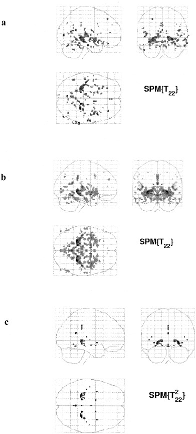
a: standard contrast, uncorrected P = 0.001; b: average contrast, uncorrected P = 0.001; c: conjunction analysis, uncorrected P = 0.001.
Figure 2 shows the position and extent of the grey matter abnormalities in the patients identified by all three analyses in the same coronal slice. The images are superimposed on the average of the normalised scans of the patients and the controls. From Figure 2 it can be seen that all three contrasts detect bilateral hippocampal effects. However, the extent of the abnormality on the left is smaller with the standard contrast (Fig. 2a) than with the average contrast (Fig. 2b). The extent of the abnormality detected in the conjunction analysis (Fig. 2c) is smaller than with both the previous contrasts because the statistical acceptance criteria are more stringent (i.e., the abnormality needs to be present on the right and on the left in the conjunction analysis).
Figure 2.

a: standard contrast, uncorrected P value = 0.001, at coordinates ‐26 ‐38 ‐2 (left is left). b: average contrast, uncorrected P value = 0.001, at coordinates ±26–38 ‐2 (left is left). c: conjunction analysis, uncorrected P value = 0.001, at coordinates ±26 ‐38 ‐2 (left is left).
The T values of the average contrast appear much higher than the T values of the conjunction contrast (see Table I). This is simply a reflection of the fact that a different T statistic is being used as the basis of inference. In the average analysis the T statistic is a single T‐value testing for the average effect. In the conjunction analysis the T value is the minimum of the two T values for each of the contrasts (1 ‐1 0 0 and 0 0 1 ‐1). This new T value has a different distribution under the null hypothesis and hence the P values differ. As a result of this, the conjunction analysis has smaller T values than the average contrast, but it yields much more significant P values.
Table I.
Location of all points significant in the conjunction analysis at the corrected level of p = 0.05 (excluding two midline points). Coordinates give the location of maxima in the Conjunction Contrast. Corresponding maxima for the other two contrasts were within 2 to 3 mm
| Label on Figure 3 |
Region | x in mm | y in mm | z in mm | Standard contrast T value | Average contrast T value | Conjunction contrast T value | Standard contrast corrected P value | Average contrast corrected P value | Conjunction contrast corrected P value |
|---|---|---|---|---|---|---|---|---|---|---|
| 1L | Hippocampus (Left) | −26 | −38 | −2 | 6.53 | 8.31 | 5.26 | 0.243 | 0.011 | 0.000 |
| 1R | Hippocampus (Right) | 26 | −38 | −2 | 6.43 | 8.31 | 5.26 | 0.281 | 0.011 | 0.000 |
| 3L | Hippocampus (Left) | −15 | −36 | 0 | 4.71 | 7.31 | 4.71 | 1.000 | 0.064 | 0.003 |
| 3R | Hippocampus (Right) | 15 | −36 | 0 | 5.72 | 7.31 | 4.71 | 0.721 | 0.064 | 0.003 |
| 5L | Hippocampus (Left) | −32 | −28 | −12 | 5.61 | 6.10 | 4.07 | 0.791 | 0.461 | 0.037 |
| 5R | Hippocampus (Right) | 32 | −28 | −12 | 4.67 | 6.10 | 4.07 | 1.000 | 0.461 | 0.037 |
| 6L | Putamen (Left) | −34 | 3 | −4 | 4.28 | 5.90 | 4.06 | 1.000 | 0.596 | 0.039 |
| 6R | Putamen (Right) | 34 | 3 | −4 | 4.18 | 5.90 | 4.06 | 1.000 | 0.596 | 0.039 |
Figure 3 demonstrates the differences between the corrected probability in the three different contrasts. All points that were significant in the conjunction analysis at the corrected level of P = 0.05 are shown. As can be seen, all the voxels in the standard analysis were less significant than in either of the two other analyses. In turn the average analysis results were less significant than the conjunction analysis at all points (there is no entry for some points as they had no corresponding maximum).
Figure 3.
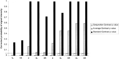
Comparison of probability values (dotted line represents significance level, P = 0.05. All the points that are significant in the conjunction analysis at the corrected significance level of P = 0.05. Points 1, 3, 5, 6 are bilateral abnormalities and 2, 4 are abnormalities in the midline). See Table I.
Further results of the conjunction analysis are shown in Figure 4. Regions that were significant at the correct 0.05 level were hippocampal (Fig. 4a and b), in the putamen (Fig. 4c) or on the sagittal midline (see below).
Figure 4.
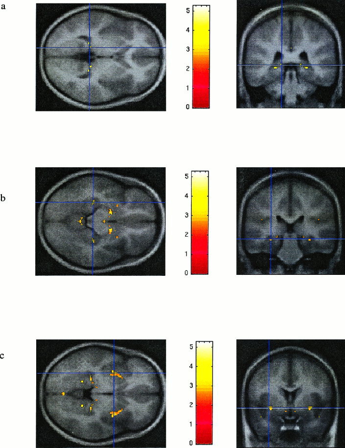
a: conjunction analysis; uncorrected P value = 0.001; ±15 ‐36 0 (left is left); bilateral hippocampus abnormality. b: conjunction analysis; uncorrected P value = 0.01; ±32 ‐28 ‐12 (left is left), bilateral hippocampus abnormality. c: conjunction analysis; uncorrected P value = 0.01; ±34 3 ‐4 (left is left), bilateral putamen abnormality.
DISCUSSION
These results demonstrate that the conjunction analysis is an improvement over the conventional analyses. The conjunction analysis has more specificity and sensitivity by virtue of employing two null hypotheses instead of one. Essentially one null hypothesis (no unilateral changes) constrains the assessment of the other (no homologous change in the other hemisphere), rendering the correction for multiple comparisons much less severe.
The conjunction analysis is therefore able to use the prior information (that bilateral abnormalities are suspected) to increase the power. This technique is clearly limited by the capability of the spatial normalisation to remove anatomical asymmetries. In regions that show great asymmetry, some bilateral deficits may be less easy to detect if that asymmetry cannot be adequately removed by spatial normalisation.
The hippocampal abnormality fits with both volumetric and standard SPM analyses and the putamen abnormality has been noted using a standard SPM approach (see Gadian et al., 2000).
All the midline abnormalities are likely to be associated with the smoothness in the data and should be discounted. This is because the data at the midline are the same in the flipped and unflipped scans, so clearly there is a higher probability of the voxels from both flipped and unflipped exceeding the threshold (i.e., a conjunction). Conjunction analyses require the contrasts to test for independent (or at least orthogonal) effects. This is violated at the midline. Only those voxels on the midline that are significant with the standard contrast should be reported. In short the conjunction analysis shows good specificity for bilateral abnormalities, although it is prone to false positives in the midline.
We are not proposing that the average contrast be used to detect bilateral abnormalities. This is because, if there were a severe unilateral effect, it is possible that this might be sufficient for the average of the flipped and unflipped differences to give rise to a significant bilateral abnormality. There is no danger of this happening in the conjunction analysis because both sides have to show an effect. In conditions such as those reviewed in the introduction it is appropriate to hypothesise bilateral abnormalities and in these cases the use of a conjunction analysis as described should be a more powerful approach.
In this example, the data were smoothed to 4 mm to sensitise the analysis to structures of a comparable size to the hippocampus, according to the matched filter theorem. The choice of smoothing kernel may impact on statistical validity: the general linear model assumes that after fitting, the residuals are normally distributed. The segmented images contain values that are mostly either zero (and slightly above), or one (and slightly below). Therefore, without any smoothing, the residuals are far from normally distributed. With more smoothing, the values are more normally distributed (by the Central Limit Theorem), and so the parametric models become more valid. It remains to be justified that smoothing to 4 mm is sufficient to prevent the violations of the assumptions of the statistical model. An alternative method is being developed by Taylor et al. [1998] (reweighted logistical regression) that addresses this issue. In summary we appeal to the Central Limit Theorem to say that the residuals will be normally distributed after spatial convolution. We are currently investigating the lower limits on spatial smoothing for the inferences to remain robust and some provisional results will be found in Ashburner and Friston [2000].
An additional concern may appear to be that large areas of grey matter may render the spatial correlations among the residuals greater than those at the cortical sheet. This however is not a problem for the analysis since inferences made in SPM99 are valid in the context of nonstationary and nonisotropic smoothness. It should also be noted that only voxels surviving a grey matter threshold (0.8) are included in the analysis. This precludes analysing areas with near‐zero variance (e.g., extracranial regions).
The general approach outlined in this article can be extended to functional characterisations. Bilateral structural lesions are not necessary to produce a severe developmental impairment. An example of this is children with Landau‐Kleffner syndrome [Landau and Kleffner, 1957]. After having acquired normal speech, these children become aphasic as a result of bilateral interference with activity in the perisylvian areas by seizures emanating, in some cases, from the auditory cortex of one temporal lobe [Morrell et al., 1995; Pateau et al., 1991]. A further example of a functional bilateral abnormality is a child, Alex, with Sturge‐Weber syndrome affecting the left hemisphere: he suffered from seizures and remained mute with a mental age of 3 or 4 until he was 8 and a half. At this point, following a left hemispherectomy, he became seizure free. Several months later he began to speak, eventually achieving a language level of an 11‐year‐old [Vargha‐Khadem et al., 1997]. It is assumed that these cases result from the functional interference or inhibition of one hemisphere by the other. In such cases it may be appropriate to look for bilateral functional abnormalities. The conjunction analysis and flipping techniques described in this article may be suitable for this purpose.
In this appendix we present the equations that give the corrected P value P n for a conjunction of effects in multiple SPMs of any statistic using (i) the unified theory described in Worsley et al. [1996] that can be applied to any specified search volume and (ii) the extension for intersections of multiple SPMs given in Cao and Worsley [1999]. A conjunction can be modelled as the intersection of the excursion sets A1, … , An of n isotropic random fields X1, … , Xn in ℜ︁D (or equivalently a single D‐dimensional field whose values comprise the minimum value of X1, … , Xn) conjointly thresholded at t. By the Poisson clumping heuristic
| (A.1) |
where ψ0 is an estimate of the expected number of maxima in the conjunction [Adler 1981; Friston et al., 1994]. The expected number of maxima is approximated by the Euler Characteristic of the conjunction and is the first component of
 |
where
 |
(A.2) |
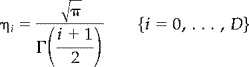
The expected diameter, area, volume etc., can be obtained from the remaining components. These expectations are functions of the Euler Characteristic (EC) densities ρi(t) and the Resel counts Rj. Both are defined for a variety of statistics in Worsley et al. [1996]. The EC densities in matrix A are a function of, and only of, the statistical value t and play a role analogous to the integral under the statistic's probability density function pdf(t) under the null hypothesis in conventional statistics (i.e., the expected number of false positives per i‐dimensional volume). For a point (i.e., one test) i = 0 and
 |
(A.3) |
The Resel counts Rj in vector b are simply the j‐dimensional volume of the search expressed in terms of resolution elements or Resels. This can be construed as a volume measure normalised by the spatial smoothness. This smoothness is estimated in the usual way, using the variances of the first partial derivatives of the statistic's component fields (in practice, the residual fields that ensue during the computation of the SPM). For a point R0 = 1 and the P value for a conjunction reduces to ρ as one might expect for a single statistical test.
As SPM99 computes the effective search volume in RESELs (i.e., resolution elements) in a way that allows for nonstationary smoothness, the results for the minimum of several t fields (i.e., a conjunction SPM) are therefore valid in the context of nonisotropic and nonstationary residuals. This is not the case for tests based on spatial extent when that extent is measured in voxels as opposed to RESELs. However, we did not use spatial extents in this article.
REFERENCES
- Adler RJ (1981): The geometry of random fields. New York: Wiley. [Google Scholar]
- Ashburner J, Friston K (1997): Multimodal image coregistration and partitioning—a unified framework. Neuroimage 6: 209–217. [DOI] [PubMed] [Google Scholar]
- Ashburner J, Friston KJ (1999): Nonlinear spatial normalisation using basis functions. Hum Brain Mapp 7: 254–266 [DOI] [PMC free article] [PubMed] [Google Scholar]
- Ashburner J, Friston KJ (2000): Voxel based morphometry—the methods. Neuroimage 11: 805–821. [DOI] [PubMed] [Google Scholar]
- Basser L (1962): Hemiplegia of early onset and the faculty of speech with special reference to the effects of hemispherectomy. Brain 85: 427–460. [DOI] [PubMed] [Google Scholar]
- Cao J, Worsley KJ. (1999): The geometry of the Hotelling's random field with applications to the detection of shape changes. Annals of Statistics 27(3): 925–942. [Google Scholar]
- Friston KJ, Worsley KJ, Frackowiak R, Mazziotta JC, Evans AC (1994): Assessing the significance of focal activations using their spatial extent. Hum Brain Mapp 1: 210–220. [DOI] [PubMed] [Google Scholar]
- Friston KJ, Ashburner J, Frith CD, Poline JB, Heather JD, Frackowiak RSJ (1995): Spatial registration and normalisation of images. Hum Brain Mapp 3: 165–189. [Google Scholar]
- Friston KJ, Holmes AP, Price CJ, Buchel C, Worsley KJ (1999): Multi‐subject fMRI studies and conjunction analyses. Neuroimage 10: 385–396 [DOI] [PubMed] [Google Scholar]
- Gadian, DG , Aicardi, J , Watkins, KE , Porter, DA , Mishkin, M , and Vargha‐Khadem F (2000): Developmental amnesia associated with early hypoxic‐ischaemic injury. Brain 123: 499–507 [DOI] [PubMed] [Google Scholar]
- Goldman PS (1979): Neuronal plasticity in primate telencephalon. Anomalous projections induced by prenatal removal of the frontal cortex. Science 202: 768–770. [DOI] [PubMed] [Google Scholar]
- Incisa della Rocchetta A, Gadian DG, Connelly A, Polkey CE, Jackson GD, Watkins KE, Johnson CL, Mishkin M, Vargha‐Khadem F (1995): Verbal memory impairment after right temporal lobe surgery: role of contralateral damage as revealed by 1H magnetic resonance spectroscopy and T2 relaxometry. Neurology 45: 797–802. [DOI] [PubMed] [Google Scholar]
- Landau WM, Kleffner FR (1957): Syndrome of acquired aphasia with convulsive disorder in children. Neurology 7: 523–530. [DOI] [PubMed] [Google Scholar]
- McCarthy RA, Warrington EK (1990): Cognitive neuropsychology: a clinical introduction. San Diego: Academic Press. [Google Scholar]
- Morrell F, Whisler WW, Smith WC, Hoeppner TJ, de Toldeo‐Morrell L, Pierre‐Louis SJC, Kanner AM, Buelow JM, Ristanovic R, Bergen D, Chez M, Hasegawa H (1990): Landau‐Kleffner syndrome: treatment with subpial intracortical transection. Brain 118: 1529–1546. [DOI] [PubMed] [Google Scholar]
- Mugler JP, Brookeman JR (1990): Three dimensional magnetisation‐prepared rapid gradient echo imaging. Magn Reson Med 15: 152–157. [DOI] [PubMed] [Google Scholar]
- Pateau R, Kajola M, Korkman M, Hamalainen M, Granstrom ML, Hari R (1991): Landau‐Kleffner syndrome: epileptic activity in the auditory cortex. Neuroreport 2: 201–204 [PubMed] [Google Scholar]
- Rasmussen T, Milner B (1977): The role of early left‐brain injury in determining lateralization of cerebral speech functions. Ann N Y Acad Sci 299: 355–369. [DOI] [PubMed] [Google Scholar]
- Richardson MP, Friston KJ, Sisodiya SM, Koepp MJ, Ashburner J, Free SL, Brooks DJ, Duncan JS (1997): Cortical grey matter and benzodiazepine receptors in malformations of cortical development. A voxel‐based comparison of structural and functional imaging data. Brain 120: 1961–1973. [DOI] [PubMed] [Google Scholar]
- Satz P, Strauss E, Wadar J, Orsini DL (1988): Acquired aphasia in children In: Sarno MT, editor. Acquired aphasia. New York: Academic Press; [Google Scholar]
- Satz P, Strauss E, Whitaker H (1990): The ontogeny of hemispheric specialization: some old hypotheses revisited. Brain Lang 38: 596–614. [DOI] [PubMed] [Google Scholar]
- Shallice T (1988): From neuropsychology to mental structure. Cambridge: Cambridge University Press. [Google Scholar]
- Sowell ER, Thompson PM, Holmes CJ, Batth R, Jernigan TL, Toga AW (1999): ) Localizing age‐related changes in brain structure between childhood and adolescence using statistical parametric mapping. Neuroimage 9: 587–97 [DOI] [PubMed] [Google Scholar]
- Taylor J, Worsley KJ, Zijdenbos AP, Paus T, Evans AC (1998): Detecting anatomical changes using logistic regression of structure masks. Neuroimage 7: S753. [Google Scholar]
- Teuber H (1975): Recovery of function after brain injury in man In: Porter R, Fitzsimmons D, editors. Outcome of severe damage to the central nervous system. Amsterdam: Elsevier Excerpta Medica, p 159–190. [Google Scholar]
- Vargha‐Khadem F, Carr LJ, Isaacs E, Brett E, Adams C, Mishkin M (1997): Onset of speech after left hemispherectomy in a nine‐year‐old boy. Brain 120: 159–182. [DOI] [PubMed] [Google Scholar]
- Vargha‐Khadem F, Isaacs E, Muter V (1994): A review of cognitive outcome after unilateral lesions sustained during childhood. J Child Neurol 9 Suppl 2: 67–73. [PubMed] [Google Scholar]
- Vargha‐Khadem F, Mishkin M (1997): Speech and language outcome after hemispherectomy in childhood In: Tuxhorn I, Holthausen H, Boenigk HE, editors. Paediatric epilepsy syndromes and their surgical treatment. London: John Libbey, p 774–784. [Google Scholar]
- Vargha‐Khadem F, Watkins KE, Price CJ, Ashburner J, Alcock KJ, Connelly A, Frackowiak RS, Friston KJ, Pembrey ME, Mishkin M, Gadian DG, Passingham RE (1998): Neural basis of an inherited speech and language disorder. Proc Natl Acad Sci U S A 95: 12695–12700. [DOI] [PMC free article] [PubMed] [Google Scholar]
- Vargha‐Khadem F, Watters GV, O'Gorman AM (1985): Development of speech and language following bilateral frontal lesions. Brain Lang 25: 167–183. [DOI] [PubMed] [Google Scholar]
- Worsley KJ (1999): Tests for conjunctions. In press.
- Worsley KJ, Marrett P, Neelin P, Vandal AC, Friston KJ, Evans AC (1996): A unified statistical approach for determining significant signals in images of cerebral activation. Hum Brain Mapp 4: 58–73. [DOI] [PubMed] [Google Scholar]
- Wright IC, McGuire PK, Poline JB, Travere JM, Murray RM, Frith CD, Frackowiak RS, Friston KJ (1995): ). A voxel‐based method for the statistical analysis of gray and white matter density applied to schizophrenia. Neuroimage 2: 244–252. [DOI] [PubMed] [Google Scholar]