A wavelet‐based approximation of surface coil sensitivity profiles for correction of image intensity inhomogeneity and parallel imaging reconstruction

Abstract

We evaluate a wavelet‐based algorithm to estimate the coil sensitivity modulation from surface coils. This information is used to improve the image homogeneity of magnetic resonance imaging when a surface coil is used for reception, and to increase image encoding speed by reconstructing images from under‐sampled (aliased) acquisitions using parallel magnetic resonance imaging (MRI) methods for higher spatiotemporal image resolutions. The proposed algorithm estimates the spatial sensitivity profile of surface coils from the original anatomical images directly without using the body coil for additional reference scans or using coil position markers for electromagnetic model‐based calculations. No prior knowledge about the anatomy is required for the application of the algorithm. The estimation of the coil sensitivity profile based on the wavelet transform of the original image data was found to provide a robust method for removing the slowly varying spatial sensitivity pattern of the surface coil image and recovering full FOV images from two‐fold acceleration in 8‐channel parallel MRI. The results, using bi‐orthogonal Daubechies 97 wavelets and other members in this family, are evaluated for T1‐weighted and T2‐weighted brain imaging. Hum. Brain Mapping 19:96–111, 2003. © 2003 Wiley‐Liss, Inc.

INTRODUCTION

Increasing the sensitivity of cortical functional magnetic resonance imaging (MRI) is desirable for either reducing the amount of inter‐subject averaging needed to detect subtle cortical activations or for increasing the spatial resolution of the mapping technique. The decrease in detected MR signal at higher resolution is confounded by an accompanying increase in the susceptibility induced spatial distortions in single shot echo planar imaging (EPI) as a percentage of the voxel dimension due to the lengthened readout. Both of these problems can be partially addressed with the use of phased array surface coil detectors, which offer the potential to both increase the MR detection sensitivity in the cortex and reduce susceptibility induced image distortions by reducing the length of the EPI readout using the SENSE method [Golay et al., 2000].

A volume birdcage head coil is conventionally used to achieve homogeneous spatial reception at loci distributed over the whole brain. However, surface coils and surface coil arrays offer the potential for an increase in sensitivity of up to 5‐fold in the cortex compared to volume coils at the expense of signal spatial homogeneity [Roemer et al., 1990; Wald et al., 1995]. While the phased array technique improves the homogeneity of the images in the plane of the array compared to a single surface coil, the image intensity is still significantly brighter near the coils than deeper in the brain. Thus, the surface coil detector has an inherently inhomogeneous reception profile that leads to a variation in image brightness across the head. This significantly degrades the utility of the images for evaluation of anatomy in the cortex and can also impair automated segmentation of brain structures. For example, in our T1‐weighed array images, the signal in the cortex near the coils is approximately 3‐fold higher than in the deep gray structures even though these gray structures have similar intensities in a uniform head coil acquisition. This difference is considerably greater than the contrast between adjacent gray and white matter whose intensities differ only by 22% in a high‐contrast T1‐weighted image.

The surface coil intensity variation is, however, a slowly varying function of position and is amenable to theoretical prediction or measurement. Once the signal intensity changes due to the coil's reception efficiency are determined, the resultant image intensity variations can be greatly reduced by dividing the original images by the coil sensitivity map. Several different methods have been described for determining the surface coil intensity profile [Axel et al., 1987; Brey and Narayana, 1988; Cohen et al., 2000; Gelber et al., 1994; Irarrazabal et al., 1996; Lai and Fang, 1999; Liney et al., 1998; Maurer et al., 1996; Mihara et al., 1998; Moyher et al., 1995; Murakami et al., 1996; Narayana et al., 1988; Roemer et al., 1990; Ross et al., 1997; Thulborn et al., 1998; Van Leemput et al., 1999; Wald et al., 1995; Zanella et al., 1990]. These methods use either a theoretically generated model [Moyher et al., 1995; Roemer et al., 1990] of the coil or the information in the image itself [Axel et al., 1987; Narayana et al., 1988] to generate the expected coil sensitivity map. In the first case, knowledge of the location and orientation of each surface coil is required in addition to a B₁ field map generated from the coil geometry. In the second case, the image variations due to coil fall‐off must be separated from those due to anatomical variations. The coil intensity profile can be approximated by a low‐pass filtered version of the original image since the coil intensity profile is generally a slowly varying function of position while the anatomic information occurs at higher spatial frequencies. This approach has been demonstrated in a number of different forms [Cohen et al., 2000; Irarrazabal et al., 1996; Van Leemput et al., 1999; Wald et al., 1995]. The low‐pass filter based approximation of the surface coil profile requires a priori knowledge of the anatomy and coil fall‐off in order to determine the appropriate cut‐off spatial frequency that separates the low‐frequency variations due to coil fall‐off from the higher spatial frequency variations arising from the anatomy.

The largest anatomical artifact incurred when estimating the coil profile based on a low‐pass filtered version of the original image originates from the air–tissue interface under the coil. This is typically the highest contrast area of the image due to its close proximity to the coil and the complete lack of signal from the air region. Furthermore, the air region is often uniform on the length scale of the low‐pass filter resulting in an underestimate of the coil map near the skin‐air boundary. Similarly, the low‐pass filtered version of the image generates a poor approximation of the coil sensitivity map near any other large low signal regions such as the lateral ventricles in T1‐weighted images. When this underestimated coil profile map is used to normalize the original image, the result is a residual brightness near the interface.

The approximation of the coil intensity profile can be improved by using a body coil image to determine anatomical content in the original image at the expense of acquisition time [Mihara et al., 1998; Thulborn et al., 1998]. If a body coil image is used, it must have a high enough spatial resolution and image contrast to allow the anatomical features of the surface coil image to be extracted. The large anatomical features such as the edge of the head can also be explicitly removed from the image prior to the low‐pass filtering [Wald et al., 1995]. This requires some a priori knowledge about the location of the high‐contrast features, thus limiting the method's robustness to unexpected features such as large cystic or contrast‐enhancing regions.

Prior to removing the spatial variations in the detected intensity of the individual array elements, it is beneficial to characterize their spatial information and use this information to decrease the acquisition time of high‐speed imaging techniques such as EPI. Recent methods that utilize the parallel nature of phased array acquisition to decrease the number of gradient encoding steps needed in the phase encode direction include k‐space domain methods such as SMASH [Sodickson, 2000; Sodickson and Manning, 1997] and image domain methods such as SENSE [Pruessmann et al., 1999]. In principle, these techniques allow the number of phase encode steps to be reduced by a factor of up to the number of elements in the phased array. The reduced number of phase encode steps (under‐sampling in k‐space) results in a “folded” or aliased image. The information from the coil sensitivity maps is then used to unfold the aliased images [Pruessmann et al., 1999; Sodickson, 2000; Sodickson and Manning, 1997]. The shorter image encoding period is beneficial for improving the spatiotemporal resolution of fMRI or reducing the susceptibility induced distortion in EPI. Thus, in brain MRI, improvements in the estimation of surface coil sensitivity profiles can be exploited for both homogeneous visualization of the image and decreased encoding times.

Here we propose a method to estimate the surface coil sensitivity profiles using only post hoc processing of the anatomical surface coil image. This coil sensitivity estimation can be utilized to correct image intensity variations, and to reconstruct full FOV images in parallel MRI for high spatiotemporal resolution brain images. The method mitigates the effect of edges in the estimation of the coil sensitivity map by using an iterative maximum value projection method to improve the approximation of the coil sensitivity profile near the edge of the head. The slowly varying intensity changes, which comprise the estimated coil sensitivity map, are determined from a filter bank implementation. This method allows the comparison of multiple levels of spatial filtering. The optimum level of filtering is determined by an automated analysis of the coil profile smoothness and the spatial variance in the corrected images.

MATERIALS AND METHODS

The images from a surface coil can be viewed as the product of the true anatomical image and a function representing the spatial modulation imposed on the image by the surface coil reception profile. Thus, the true homogeneous image, C[ ], is modulated by the coil sensitivity, S[], to generate the observed inhomogeneous image, Y[], where is the position vector in 3‐D space. Thus our goal is to get an estimate, [] of the true coil sensitivity profile, S[]. The intensity‐corrected reconstruction image, [], which represents an approximation of the true anatomical image, is then expressed in terms of the ratio of the original data and the estimated coil sensitivity profile.

(1)

If aliased images are acquired in order to reduce encoding time, an unfolded image is generated by inverting the folding process which is represented by a kspace under‐sampling matrix. Since k‐space is under‐sampled, the additional spatial information available from the multiple receive channels is needed to complete the matrix inversion. We have applied the standard SENSE reconstruction method and generated a G‐factor map depicting the noise added in the unfolding process [Pruessmann et al., 1999]. The surface coil intensity profile [] from the measured image is used as an input for the SENSE unfolding method.

Multi‐Resolution Analysis

We estimate the coil intensity profile using a hierarchical filter bank structure to efficiently implement a Multi‐Resolution Analysis (MRA) [Daubechies, 1992; Strang and Nguyen, 1996; Vaidyanathan, 1993] of the original inhomogeneous MRI. In general, MRA decomposes the image into a series of orthogonal “coarse approximations” sub‐space and “fine details” sub‐space at different spatial resolutions. After breaking down the image into sub‐components of different resolution, the original image can be regenerated from the direct sum of the sub‐images if desired [Daubechies, 1992; Strang and Nguyen, 1996]. When applied to discrete images, this method is referred to as the discrete‐time wavelet transform, DWT [Vaidyanathan, 1993].

In estimating coil sensitivity profiles with the iterative analysis low‐pass filter bank, the cut‐off spatial frequencies are progressively lowered until very little spatial information is left in the image. Since the coil sensitivity map consists of the slowly varying sensitivity profile of the coil and the details subspace likely contains mainly anatomical information, we estimate S[ ] from the low‐pass filter data only. This estimate of the coil sensitivity map is computed at each level of the MRA.

In implementation, we use the bi‐orthogonal maximally‐flat Daubechies' wavelet and scaling functions [Daubechies, 1992; Strang and Nguyen, 1996]. The property of symmetric wavelet and scaling functions of this implementation avoids any pixel shift in the filtered data. Also, the Daubachies' bi‐orthogonal wavelet family allows the choice of the number of vanishing moments in the filter. This determines the number of zeroes of the discrete digital filters' spectrum; more zeroes provide a higher approximation accuracy. Specifically, we chose Daub97 bi‐othorgonal filter banks in our studies. In this notation, the first digit represents the length of analysis filter, which is also the support of the analysis scaling/wavelet function. The second digit describes the length of synthesis filter bank. Daub97 filter banks have 3 zeros at π for the low‐pass filter in synthesis filter bank. Thus, their approximation power for signal reconstruction is equal to cubic polynomials at each spatial scale.

Application to Coil Sensitivity Profile Estimation

While a given level of the MRA of the original surface coil image could be used alone to estimate the coil sensitivity profile, this leads to an underestimation of the coil sensitivity map in the vicinity of high‐contrast edges in a similar manner to other low‐pass filter based estimates. These high‐contrast features may arise from anatomy inside the brain (e.g., ventricles) or from the air‐skin interface. To address this problem, we use an iterative process to improve the estimation near the high‐contrast edge. This method is applied to each level of the multiple resolution analysis. The generation of the coil sensitivity map at a given MRA level is formed by taking the maximum value projection (MVP) of the approximation subspace (low spatial frequency information) generated by the MRA with the original image. The maximum value projection of two input images is an image whose pixel values are the pixel by pixel maximum of the two input images. Thus, the intensity of a given pixel in the maximum value projection image is defined to be that of the greater of the two corresponding pixels in the two input images. In order to form the coil sensitivity estimate from a given level of the MRA, the MRA and maximum value projection are repeated iteratively. In this process, the MVP of the output of the MRA and the original image is re‐analyzed with the MRA method at a given level. The result of the MRA is then re‐compared with the original image using MVP and the output is re‐analyzed with MRA at the same level. Thus, the input for the (i+1th application of the discrete wavelet transform is generated from a maximum value projection of the current result (ith iteration) and the original image. The process is outlined in Figure 1. We stop the iteration when the total power in the difference image formed from two consecutive iterations is less than 1% of the power in the current iteration.

Figure 1.

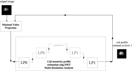
Schematic diagram of the iterative estimation of coil sensitivity profile at a specific level l by Discrete‐time Wavelet Transform (DWT) based on the Maximum Value Projection (MVP) of the previous estimate and the original inhomogeneous input raw image. LP0 denotes the cascade of a low‐pass filter and a two‐fold down‐sampler. LP1 denotes the cascade of two‐fold up‐sampler and synthesis low‐pass filter.

The iterative MVP process reduces the underestimation of the signal at a high contrast interface (such as the brain‐air boundary). An example using one‐dimensional data is illustrated in Figure 2. The projection helps to preserve the original high pixel intensity on the bright side of an edge while increasing the pixel intensity on the darker side of a high contrast edge. The process has the effect of filling in the low‐signal intensity regions in a smooth fashion while preserving the local maximum on the tissue side of the interface. Thus, for the edge of the head, the accuracy of the coil map is improved on both sides of the interface. Once the iterative maximum value projection process converges for a given level of MRA, the process is repeated at the next level. Thus, for an image matrix of 2 ⁿ, n levels of the coil sensitivity profile estimates are generated, each at a different spatial resolution. Each level of estimation employs both the DWT and maximum value projection. Any of these levels of MRA estimation could, in principal, be used as [] to either generate the corrected version of the original image, or to reconstruct full‐FOV images in parallel MRI.

Figure 2.

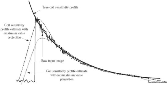
Simulation of one‐dimensional data (thin solid line) with superimposed slowly varying trend (thick solid line) and signal from anatomical contrast. The sharp edge is a simulation of the abrupt signal change at an anatomical boundary such as the air‐scalp interface. The first estimation (dotted line) without maximum projection underestimates the sensitivity at the boundary. Iterative maximum projection of the previous estimate and the original data (dashed line) provides a better approximation of the global trend in the data, especially in the brain region near the boundary.

Automatic Selection of Optimal Reconstruction Level

For an image matrix of 2 ⁿ, the wavelet‐based method provides n distinct coil sensitivity profiles at different levels of spatial smoothing. For each level, an inhomogeneity‐corrected image can be obtained by pixel‐by‐pixel quotient of the original image over the estimated profile pattern. Automatic selection of the optimal reconstruction level can be achieved by defining a metric of how well the algorithm has done at removing the variance in the image due to the coil profile. This metric cannot be a simple measure of image variance since image variance is minimized when both the coil profile and the fine spatial scale anatomic variations are removed from the image. Qualitatively, the optimal reconstruction would contain a high contrast between parenchymal tissue types and low pixel value variance within individual structures. Additionally, the estimated coil sensitivity profile is expected to be spatially smooth due to the electromagnetic properties and the topologies of the coil. We defined an “inhomogeneity index”, I _l, as a metric of how well the algorithm removes the coil profile at each level l. The MRA level, which generates a corrected image with the minimum inhomogeneity index, is chosen as the best approximation of the coil profile. The index is a product that attempts to minimize variance V _l within a loosely defined tissue type, and maximize the smoothness θ _l of the coil map and contrast C _l between tissue types

(2)

Here V _l denotes the pixels intensity variability within a tissue type in the reconstructed anatomical image at spatial level l. And C _l denotes the contrast between tissue types in the reconstructed anatomical image. θ _l is an estimate of the spatial smoothness of the estimated coil sensitivity profile. Thus, the inhomogeneity index is computed from both the corrected image and estimated coil profile generated at each spatial level. We use the Gaussian Mixture Model (GMM) [Redner and Walker, 1984; Titterington et al., 1985] to categorize the intensity histogram of the reconstructed images. In GMM, the pixel intensity histogram of an image is assumed to follow multiple Gaussian distributions, each of which is characterized by the unknown mean μ_k, variance Σ_k and probability p _k. The probability of a pixel with value ζ is written:

(3)

GMM parameters p _k, μ_k, Σ_k can be calculated using Expectation‐Maximization (EM) algorithm [Axel et al., 1987; Redner and Walker, 1984]. The variance in the corrected image, V _l, is calculated as the sum of all variances (Σ_k) of the Gaussian models, and the contrast of the corrected image, C _l, is the difference between the Gaussian distributions with the lowest and the highest mean value as a metric of image contrast. We evaluated the use of 2 to 6 Gaussians in our model. Using 3 Gaussian distributions in T1‐weighted images, the histogram of the corrected anatomical image at the optimal level can be approximately partitioned into gray matter, white matter, and scalp lipids. The spatial smoothness of the coil θ _l is calculated by convoluting a 3‐pixel × 3‐pixel discrete Laplacian operator over the estimated coil sensitivity profile and summing the pixel values of the resulting map [Lim, 1990].

Image Acquisition for Image Intensity Inhomogeneity Removal

Images were acquired using a 3T scanner (Siemens Medical Solutions, Iseln, NJ) with a home‐built two‐ or four‐element bilateral surface coil array. The array elements consisted of 9‐cm–diameter surface coils. The imaging pulse sequence was a T1‐weighted MPRAGE 3‐D volume exam (TR/TE/TI/flip = 2,530 msec/3.49 msec/1,100 msec/7 degrees), partition thickness = 1.33 mm, matrix = 256 × 256, 128 partitions, Field of View = 21 × 21 cm or a T2‐weighted Turbo Spin Echo (TSE) sequence (TR/TE/flip = 6,000 msec/97 msec/160 degrees, slice thickness = 3 mm, matrix = 512 × 448, Field of View = 22 × 19.2 cm). The 3‐D images were cropped to 256 × 204 matrix size to minimize the background airspace for visualization purpose before inhomogeneity correction. The array elements were placed over the subject's temporal lobes. To compare the corrected surface coil image with a uniform coil, the nearest anatomical slice prescription and imaging parameters were applied to a birdcage head coil. The utility of the image correction algorithm for rendering surface coil images suitable for automated segmentation algorithms was tested by using the FreeSurfer [Fischl et al., 1999; online at http://surfer.mgh.harvard.edu] segmentation package. Both the original and intensity corrected 3‐D T1‐weighted isotropic 1‐mm resolution MPRAGE images were processed.

Parallel MRI Acquisition and Reconstruction

For parallel MRI acquisition and reconstruction, a home‐built 8‐channel 3T head array consisting of a linear array of 9‐cm–diameter circular surface coils wrapped around the head was used to test the algorithm for SENSE parallel image reconstruction. Images were under‐sampled in the phase‐encode direction by 50% (skipping every other phase‐encoding line) to achieve two‐fold acceleration. A T1‐weighted FLASH sequence (TR/TE = 450 msec/12 msec, slice thickness = 3 mm, matrix = 256 × 256, Field of View = 19 × 19 cm) was used with axial slices through the brain. Given the estimated coil sensitivity maps from each coil acquired with a full FOV reference image, the aliased images were unfolded using a standard SENSE approach [Sodickson and McKenzie, 2001]. Noise amplification from the geometrical arrangement of the array coil elements is calculated by the G‐factor map [Pruessman et al., 1999].

RESULTS

The original 256 × 204 × 128 uncorrected 3‐D T1 images were corrected to give six distinct coil profile estimations at six spatial scales. In the uncorrected image (Fig. 3), white matter signal intensity is 280% higher near the coils than deeper in the brain. This wide variation in image intensity arises primarily from the coil reception profile. Adjacent gray and white matter regions differ by only 22%. Thus, the coil's reception profile makes most of the anatomy difficult to visualize with a single window and level setting.

Figure 3.

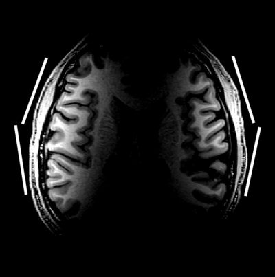
The raw image acquired from bilateral phased array. White bars, the approximate location of the elements of the array.

Figure 4 shows the estimated sensitivity profiles derived from Daubechies‐97 (Daub97) filter bank and maximum value projection at each level (1 to 6). The corrected images obtained from each level are shown in Figure 5. Reconstruction using level 1, 2, or 3 fails to preserve the local brain structures because the estimated profile includes anatomical features that are then partially removed during the division step (Eq. 1). Level 6 coil profile is too spatially smoothed to effectively remove the coil intensity effects. Each level of corrected image required an average of 4.73 sec of computation per level for a 256 × 204 image slice using a 450‐MHz processor (Intel Pentium III; Santa Clara, CA).

Figure 4.

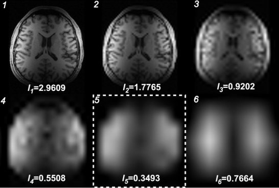
Estimated sensitivity profiles and inhomogeneity indices for each of the 6 levels (1) of wavelet decomposition and reconstruction. Level 5 (boxed by white dashed line) was found to provide the optimal estimation based on the inhomogeneity index I_l.

Figure 5.

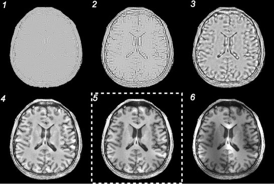
Six levels of correction by Daub97 filter bank. Reconstruction at level 5 (boxed by white dashed line) provided the optimal reconstruction based on a minimization of the inhomogeneity index.

The optimum level used to estimate the coil sensitivity profile was determined by the quantitative inhomogeneity index in Eq. 2. The indexes computed with a 3 Gaussian GMM are shown in Figure 4. Level 5 provided the minimum inhomogeneity index of the 6 levels regardless of the whether 2, 3, 4, 5, or 6 Gaussians were used in the GMM. After correction, visualization of deep sub‐cortical structures is considerably improved. The visibility for gray and white matter as well as the contrast between them is maintained for both cortex and deep gray structures at the same window and level. The reconstructed image contained peak‐to‐peak value white matter differences of 39% compared with differences of 280% in the original image. When the T1‐weighted volumetric images were processed with the automated segmentation algorithm, the image intensity normalization was found to be sufficient to allow automated segmentation while the unprocessed surface coil images could not be processed with this package.

The maximum value projection was found to significantly improve the coil profile estimation near high‐contrast edges. Figure 6 shows one‐dimensional profile of the original image through the third ventricle and the coil sensitivity profile estimates with and without maximum value projection overlaid. The coil profile generated from a non‐iterative, low‐pass filter–based approach is also overlaid. The low‐pass filter consisted of a 26‐mm (32 × 32 pixel) moving‐average low‐pass kernel filter. This level of spatial smoothing is roughly equivalent to that of the level 5 MRA. Omission of the MVP step resulted in a 50% underestimation of the image data at the edge of the brain. Adding the MVP algorithm with a 1% convergence criteria reduced this error to approximately 5%. Less than five iterations of the MVP were required for convergence with a 1% criteria for each spatial level of the MRA. The convergence times for a given level of the wavelet‐based method with and without the MVP step were a maximum of 6.7 and 2.3 sec, respectively.

Figure 6.

A cross‐section from the unprocessed image data at the location of the 3rd ventricle (solid line) overlaid with the sensitivity profile estimate without maximum intensity projection (MVP) (dotted line), and the sensitivity profile with MVP (thick dashed line). Without iterative MVP, the coil sensitivity profile is under‐estimated at the brain‐air boundary, as predicted in the simulation (shown in Fig. 2). MVP alleviates the underestimation and is more precise at the sharp contrast boundary. Also overlaid is a coil intensity profile estimation using a moving‐average (MA) low‐pass filter with a 32×32 pixel kernel (thin dashed line).

Figures 7 and 8 compares a standard birdcage head coil image with the corrected surface coil image. The uncorrected phased array image temporal lobe white matter SNR ranged from 351 to 466% higher than in the volume head coil birdcage image. For midline structures such as the corpus collosum, the gain was 27%. Figure 9 shows application of the method to T2‐weighted images.

Figure 7.

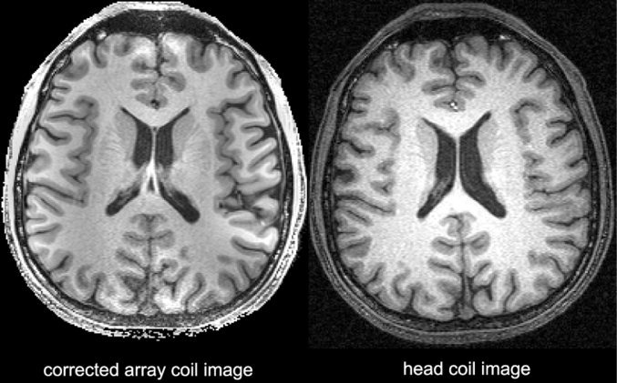
Comparison of corrected phased array image (left) and volume head coil image (right). The advantage of phased array acquisition for higher SNR at regions near to the array coil is observed. The contrast of the white and gray matter is improved and maintained relatively constant compared to the original array coil image (Fig. 3). The inhomogeneity reduction on the array coil image using DWT and maximal value projection even improves the visibility of the deep brain areas at comparable contrast to the head coil image.

Figure 8.

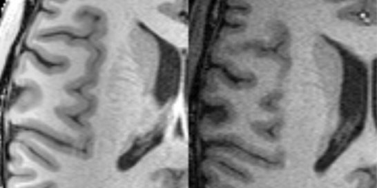
The detail of the temporal lobe from the corrected phased array surface coil image (left) and the birdcage head coil image (right).

Figure 9.

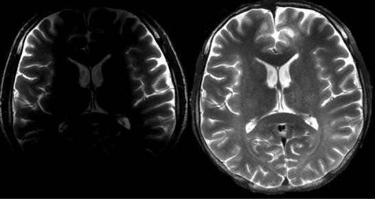
Application of the DWT estimation of coil sensitivity profile and MVP to a T2‐weighted image for inhomogeneity correction. The 2‐channel array coil was placed at the bi‐temporal lobe. The uncorrected image appears on the left. The corrected image (right) shows more details at the deep brain compared to the original one.

Figure 10 shows the application of the DWT‐generated coil intensity profiles to the generation of coil sensitivity maps of the individual array coils for parallel reconstruction applications. The coil maps are well matched to the high‐sensitivity regions of the anatomical images. The reconstructed full‐FOV image from a two‐fold under‐sampled (aliased) image is shown in Figure 11. Note that the SNR of the SENSE reconstructed image is at most 71% of the original full‐FOV reference image, because only 50% of the original k‐space data was acquired. The further amplification of noise in the SENSE reconstruction is described by the G‐factor map shown in Figure 11. The average G‐factor over the whole FOV is 1.15 with a standard deviation of 0.0952. Maximal G‐factor is 1.43, minimal G‐factor is 1.0, and the median of G‐factor is 1.14.

Figure 10.

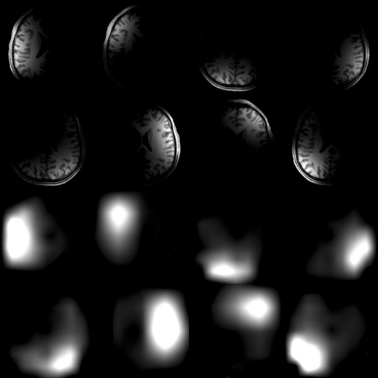
The full‐FOV reference images from an 8‐channel array coil (top) and their optimal sensitivity profile estimates (bottom) using DWT and MVP. The sensitivity profiles correlate well to the individual coil locations.

Figure 11.

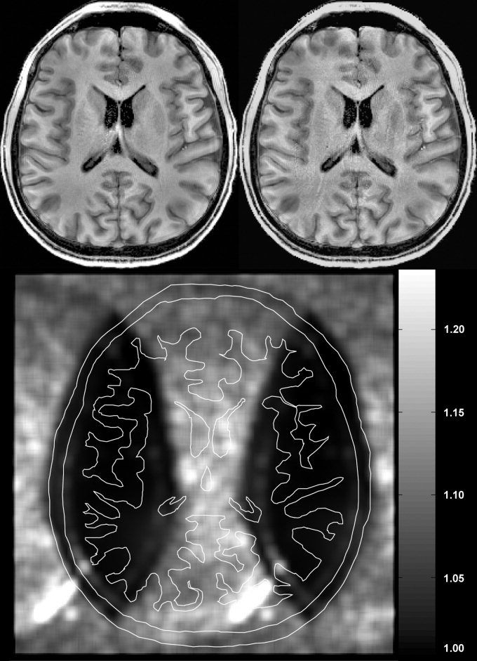
Inhomogeneity corrected full‐FOV image from an 8‐channel array coil (left) and SENSE acquisition with acceleration of 2.0 (right). Standard SENSE reconstruction was used to unfold the aliased images using information from all 8 channels in the array. The degraded SNR in the SENSE acquisition is mainly due to subsampling of k‐space data by half. Additionally, noise is added during the SENSE reconstruction. The magnitude and spatial distribution of this noise is shown in the G‐factor map (bottom). An outline of the brain anatomy is overlaid on the G factor map to show the location of the brain.

DISCUSSION

Improving the sensitivity and encoding time constraints of structural and functional brain imaging is essential for revealing the physiological processes in cognitive, sensory and motor systems. Development of high‐field scanners and improved brain array coils offer the potential to increase the resolution and sensitivity of non‐invasive MR imaging methods. Body coil or volume head (birdcage) coils provide highly homogeneous MR images. However, the SNR of volume coils in cortical regions is lower than that of surface coils. The image inhomogeneity from surface coils, however, compromises its application in functional imaging because of the intrinsic wide variation of image brightness arising from the coil sensitivity profile. In addition to making the images hard to visualize, the wide dynamic range of the surface coil image confounds the use of automated segmentation measurements of cortical parameters such as thickness and curvature or the automated identification of deep gray structures [Dale et al., 1999]. If the image inhomogeneity issue is overcome, these applications could potentially benefit from the improved resolution available from the 3–4‐fold increase in cortical sensitivity of the arrays compared to volume coils since the cortex is relatively poorly resolved on standard (1‐mm resolution) structural MRIs.

Array coils are also valuable for decreasing the magnetic field susceptibility distortion in functional imaging by allowing the reconstruction of echo‐planar images with reduced encoding times. The susceptibility induced distortion becomes especially problematic for high‐field (3T and above) studies since the susceptibility effect scales with field strength. The application of parallel imaging methods enables the accelerated image acquisition when multiple receivers are available and, therefore, a proportional reduction in susceptibility distortion. An estimate of the coil profile is a prerequisite for most of these methods. We show that the wavelet‐based estimation method can provide this estimate for the reconstruction of two‐fold accelerated SENSE images.

One of the significant features of this method is the iterative maximal value projection (MVP) at each level in multi‐resolution analysis of the anatomical image. This method was found to be fast, robust in convergence, and improve the estimate of the coil map near the high contrast air‐scalp interface. Without the MVP step, the wavelet transform estimation of the coil profile underestimated the coil profile data by 50% at the edge of the brain. Adding the MVP algorithm with a 1% convergence criteria reduced this error to approximately 5%. While we demonstrate the MVP method in conjunction with a multi‐resolution wavelet analysis to generate the low‐pass filtered image, the iterative MVP approach could be used with other low‐pass filter types in order to reduce the underestimation of the coil sensitivity profile near sharp contrast boundaries.

To select the optimal level of the coil sensitivity profile estimation using MRA, we propose a metric of the inhomogeneity index at each spatial level by using measures from the estimated coil sensitivity profile and the inhomogeneity corrected anatomical image. While other metrics might be possible, this method was found to provide the level that subjective analysis of the images would have chosen. The automated method worked for both 2‐D and 3‐D images of both T1 and T2 contrast and was found to be insensitive to the number of Gaussians used in the model. While for a certain range of image parameters it might be possible to choose the MRA level 5 based on prior knowledge of 256 matrix images and the coil used, the use of the more general approach does not increase the processing time significantly.

The proposed methods were tested in this study on a 3T MRI scanner using three different configurations of phased array coils (2‐channel, 4‐channel, and 8‐channel) for images of T1‐ and T2‐weighted contrasts to test the robustness of the wavelet‐based approach across image contrast and coil geometries. Since the goal of surface coil imaging is increased sensitivity and resolution, the study concentrated on 3T images. We have also applied the method to 1.5T images (not shown here) with similar results.

In addition to the Daub97 filter banks, which can approximate the input image with precision of the third order approximation at different spatial scales, we also employed other shorter filters of the same filter family to test the different performances. Potentially, shorter filters can save computational time. Using the T2‐weighted image in Figure 9, Figure 12 shows the coil sensitivity estimates and corrected images obtained from Daubechies 53, 75, and 97 bi‐orthogonal filter banks. All the filter implementations improve the visualization of the image by showing both cortical and deep brain structures such as the basal ganglia with a single window and level parameter. In all cases, level 5 gives the best coil sensitivity estimation. Although the coil sensitivity estimates obtained from the three filter banks are similar in many respects, there are differences. Because the Daub53 synthesis filter bank has support of 3 and 1 vanishing moment at π, the approximation ability of this filter bank is linear functions. Since the surface coil profile drops off faster than linear, the Daub53 filter results in a poorer approximation and produces a highly peaked shape in the estimated sensitivity map with a cross‐like artifact. Daub75 and Daub97 have 2 and 3 vanishing moments at π in the synthesis filter bank. This enables corresponding scaling functions to have better approximation to the smooth drop‐off of the surface coil.

Figure 12.

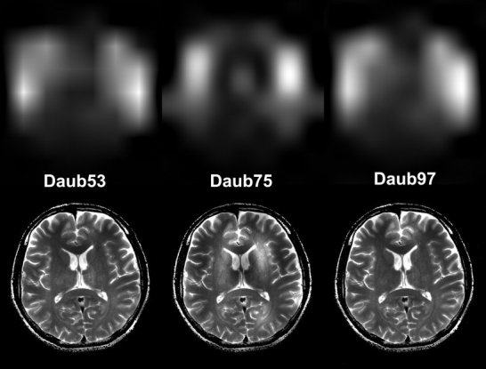
Coil sensitivity map estimations (top) and reconstruction (bottom) using Daub53 filter bank (left), Daub75 filter bank (middle), and Daub 97 filter bank (right).

The accuracy of coil sensitivity estimation has been estimated by analyzing intensity deviations over structures that are known to be homogeneous, such as white matter. An alternative approach is to compare to a theoretical estimation. While a simple Biot‐Savart type B1 field calculation works reasonably well for a single loop coil [Moyher et al., 1995], the geometry of the array is more complicated to describe. This is especially true of the semi‐flexible arrays used in this work. A major confound is the coupling between array elements. This is modulated by both coil geometry, coil loading on the body, and electrical interactions with the preamplifiers. The coupling matrix of the 8‐channel array has 28 parameters that depend on how the coil is flexed and how it is placed on the head as well as geometry and preamplifier tuning. All of these factors make it impractical to simply measure these couplings on the bench. In the absence of direct measurement, a realistic model would have too many free parameters to be useful for comparison. Additionally, dielectric effects in the head at 3T are significant (on the 30% level) requiring a full Maxwell equation simulation. While these have been performed for idealized birdcage coils, we are not aware of simulations for surface coil arrays.

Recently, the promising parallel MRI techniques [Pruessmann et al., 1999; Sodickson and Manning, 1997; Sodickson and McKenzie, 2001] enable accelerated image acquisition when multiple receivers are available. The reconstruction of full‐FOV image depends on the estimation of coil sensitivity modulation. Using our method, the reconstruction of reduced‐FOV images from multiple receivers is feasible. Coupling with the regularization technique, we demonstrated initial results of robust parallel MRI reconstruction for brain imaging when our sensitivity profile estimation technique is utilized [Lin et al., 2002]. Thus, the proposed algorithm is demonstrated for either the accelerated image acquisition or the enhanced spatial resolution using parallel MRI acquisition. The proposed methods were tested in this study in a 3T MRI scanner using 3 different configurations of phased array coils (2‐channel, 4‐channel, and 8‐channel) for images of T1‐ and T2‐weighted contrasts to test the robustness of the wavelet‐based approach across the coil position, sizes, and geometries.

In this study, we proposed a dyadic wavelet decomposition of original surface coil image to estimate the coil sensitivity map. This multi‐stage approach is equivalent to an iterative low‐pass filtering, with the cut‐off frequency at the current spatial resolution equal to half of the highest frequency in the previous spatial resolution. This division in frequency might be further improved by wavelet packet algorithm [Strang and Nguyen, 1996], which divides the input image into both high‐pass and low‐pass bands at all spatial resolutions. The wavelet packet approach allows for finer division of cut‐off frequency at the cost of increased computation time. However, this can be combined with a priori knowledge about the feasible resolution informed by dyadic DWT to locate the possible “optimal” spatial resolution. The subsequent finer division of spatial resolution might provide even more precise coil sensitivity profile estimation. This will be the research topic in the near future.

CONCLUSION

We have demonstrated an automatic method to estimate the coil sensitivity profile and use it to correct the inhomogeneity of surface coil MRI using wavelet transforms as well as for parallel imaging reconstruction using SENSE. The Daubechies maximally flat filter bank was found to have good computational efficiency and approximation of coil sensitivity map. The optimum level could be automatically determined by the defined inhomogeneity index from the corrected image and estimated coil profile. Thus, the method uses neither presumed digital filter specifications nor the knowledge of the electromagnetic properties and the location of the RF coil. Reconstructed images show both cortical and sub‐cortical structures farther away from the surface coil with relatively constant contrast. The corrected surface coil images have both higher SNR than volume coil images and homogeneous contrast and brightness. Surface coil images corrected in this way were found to be usable with automated image segmentation software. The coil sensitivity profile estimation was applied to the accelerated parallel MRI of brain images using an 8‐channel array coil to reduce the image encoding time by a factor of 2, allowing for either reduction of susceptibility distortions or increased spatial resolution at the given imaging time.

REFERENCES

- Axel L, Costantini J, Listerud J (1987): Intensity correction in surface‐coil MR imaging. AJR Am J Roentgenol 148: 418–420. [DOI] [PubMed] [Google Scholar]
- Brey WW, Narayana PA (1988): Correction for intensity falloff in surface coil magnetic resonance imaging. Med Phys 15: 241–245. [DOI] [PubMed] [Google Scholar]
- Cohen MS, DuBois RM, Zeineh MM (2000): Rapid and effective correction of RF inhomogeneity for high field magnetic resonance imaging. Hum Brain Mapp 10: 204–211. [DOI] [PMC free article] [PubMed] [Google Scholar]
- Dale AM, Fischl B, Sereno MI (1999): Cortical surface‐based analysis. I. Segmentation and surface reconstruction. Neuroimage 9: 179–194. [DOI] [PubMed] [Google Scholar]
- Daubechies I (1992): Ten lectures on wavelets, Society for Industrial and Applied Mathematics, Philadelphia, PA. [Google Scholar]
- Fischl B, Sereno MI, Dale AM (1999): Cortical surface‐based analysis. II: Inflation, flattening, and a surface‐based coordinate system. Neuroimage 9: 195–207. [DOI] [PubMed] [Google Scholar]
- Gelber ND, Ragland RL, Knorr JR (1994): Surface coil MR imaging: utility of image intensity correction filte. AJR Am J Roentgenol 162: 695–697. [DOI] [PubMed] [Google Scholar]
- Golay X, Pruessmann KP, Weiger M, Crelier GR, Folkers PJ, Kollias SS, Boesiger P (2000): PRESTO‐SENSE: an ultrafast whole‐brain fMRI technique. Magn Reson Med 43: 779–786. [DOI] [PubMed] [Google Scholar]
- Irarrazabal P, Meyer CH, Nishimura DG, Macovski A (1996): Inhomogeneity correction using an estimated linear field map. Magn Reson Med 35: 278–282. [DOI] [PubMed] [Google Scholar]
- Lai SH, Fang M (1999): A new variational shape‐from‐orientation approach to correcting intensity inhomogeneities in magnetic resonance images. Med Image Anal 3: 409–424. [DOI] [PubMed] [Google Scholar]
- Lim JS (1990): Two‐dimensional signal and image processing. New York: Prentice Hall, [Google Scholar]
- Lin F‐H, Kwong KK, Chen Y‐J, Belliveau JW, Wald LL (2002): Reconstruction of sensitivity encoded images using regularization and discrete time wavelet transformation estimates of the coil maps. Proc Intl Soc Mag Reson Med: 2389. [Google Scholar]
- Liney GP, Turnbull LW, Knowles AJ (1998): A simple method for the correction of endorectal surface coil inhomogeneity in prostate imaging. J Magn Reson Imag 8: 994–997. [DOI] [PubMed] [Google Scholar]
- Maurer CR Jr, Aboutanos GB, Dawant BM, Gadamsetty S, Margolin RA, Maciunas RJ, Fitzpatrick JM (1996): Effect of geometrical distortion correction in MR on image registration accuracy. J Comput Assist Tomogr 20: 666–679. [DOI] [PubMed] [Google Scholar]
- Mihara H, Iriguchi N, Ueno S (1998): A method of RF inhomogeneity correction in MR imaging. Magma 7: 115–120. [DOI] [PubMed] [Google Scholar]
- Moyher SE, Vigneron DB, Nelson SJ (1995): Surface coil MR imaging of the human brain with an analytic reception profile correction. J Magn Reson Imag 5: 139–144. [DOI] [PubMed] [Google Scholar]
- Murakami JW, Hayes CE, Weinberger E (1996): Intensity correction of phased‐array surface coil images. Magn Reson Med 35: 585–590. [DOI] [PubMed] [Google Scholar]
- Narayana PA, Brey WW, Kulkarni MV, Sievenpiper CL (1988): Compensation for surface coil sensitivity variation in magnetic resonance imaging. Magn Reson Imag 6: 271–274. [DOI] [PubMed] [Google Scholar]
- Pruessmann KP, Weiger M, Scheidegger MB, Boesiger P (1999): SENSE: sensitivity encoding for fast MRI. Magn Reson Med 42: 952–962. [PubMed] [Google Scholar]
- Redner RA, Walker HF (1984): Mixture densities, maximum likelihood and the Em algorithm. SIAM Rev 26: 195–239 [Google Scholar]
- Roemer PB, Edelstein WA, Hayes CE, Souza SP, Mueller OM (1990): The NMR phased array. Magn Reson Med 16: 192–225. [DOI] [PubMed] [Google Scholar]
- Ross BD, Bland P, Garwood M, Meyer CR (1997): Retrospective correction of surface coil MR images using an automatic segmentation and modeling approach. NMR Biomed 10: 125–128. [DOI] [PubMed] [Google Scholar]
- Sodickson DK (2000): Tailored SMASH image reconstructions for robust in vivo parallel MR imaging. Magn Reson Med 44: 243–251. [DOI] [PubMed] [Google Scholar]
- Sodickson DK, Manning WJ (1997): Simultaneous acquisition of spatial harmonics (SMASH): Fast imaging with radiofrequency coil arrays. Magn Reson Med 38: 591–603. [DOI] [PubMed] [Google Scholar]
- Sodickson DK, McKenzie CA (2001): A generalized approach to parallel magnetic resonance imaging. Med Phys 28: 1629–1643. [DOI] [PubMed] [Google Scholar]
- Strang G, Nguyen T (1996): Wavelets and filter banks. Wellesley: Cambridge Press, [Google Scholar]
- Thulborn KR, Boada FE, Shen GX, Christensen JD, Reese TG (1998): Correction of B1 inhomogeneities using echo‐planar imaging of water. Magn Reson Med 39: 369–375. [DOI] [PubMed] [Google Scholar]
- Vaidyanathan PP (1993): Multirate systems and filter banks. New York: Prentice Hall. [Google Scholar]
- Van Leemput K, Maes F, Vandermeulen D, Suetens P (1999): Automated model‐based bias field correction of MR images of the brain. IEEE Trans Med Imag 18: 885–896. [DOI] [PubMed] [Google Scholar]
- Wald LL, Carvajal L, Moyher SE, Nelson SJ, Grant PE, Barkovich AJ, Vigneron DB (1995): Phased array detectors and an automated intensity‐correction algorithm for high‐resolution MR imaging of the human brain. Magn Reson Med 34: 433–439. [DOI] [PubMed] [Google Scholar]
- Zanella FE, Lanfermann H, Bunke J (1990): [ Automatic correction of the signal intensity of surface coils. Clinical application and relevance. French language]. Radiologe 30: 223–227. [PubMed] [Google Scholar]