Fast robust automated brain extraction

Abstract

An automated method for segmenting magnetic resonance head images into brain and non‐brain has been developed. It is very robust and accurate and has been tested on thousands of data sets from a wide variety of scanners and taken with a wide variety of MR sequences. The method, Brain Extraction Tool (BET), uses a deformable model that evolves to fit the brain's surface by the application of a set of locally adaptive model forces. The method is very fast and requires no preregistration or other pre‐processing before being applied. We describe the new method and give examples of results and the results of extensive quantitative testing against “gold‐standard” hand segmentations, and two other popular automated methods. Hum. Brain Mapping 17:143–155, 2002. © 2002 Wiley‐Liss, Inc.

INTRODUCTION

There are many applications related to brain imaging that either require, or benefit from, the ability to accurately segment brain from non‐brain tissue. For example, in the registration of functional images to high resolution magnetic resonance (MR) images, both fMRI and positron emission tomographic (PET) functional images often contain little non‐brain tissue because of the nature of the imaging, whereas the high resolution MR image will probably contain a considerable amount, eyeballs, skin, fat, muscle, etc., and thus registration robustness is improved if these non‐brain parts of the image can be automatically removed before registration. A second example application of brain/non‐brain segmentation is as the first stage in cortical flattening procedures. A third example is in brain atrophy estimation in diseased subjects; after brain/non‐brain segmentation, brain volume is measured at a single time point with respect to some normalizing volume such as skull or head size; alternatively, images from two or more time points are compared, to estimate how the brain has changed over time [Smith et al., 2001, 2002]. Note that in this application, tissue‐type segmentation is also used to help disambiguate brain tissue from other parts of the image such as CSF [Zhang et al., 2001]. A fourth application is the removal of strong ghosting effects that can occur in functional MRI (e.g., with echo planar imaging [EPI]). These artefacts can confound motion correction, global intensity normalization, and registration to a high‐resolution image. They can have an intensity as high as the “true” brain image, preventing the use of simple thresholding to eliminate the artefacts, whereas the geometric approach presented here can remove the effects (though only from outside of the brain).

This article describes a complete method for achieving automated brain/non‐brain segmentation. The method described here does not attempt to model the brain surface at the finest level, for example, following sulci and gyri, or separating cortex from cerebellum. This finer modeling would be a later stage, if required, after the brain/non‐brain segmentation.

After a brief review of brain extraction, the brain extraction algorithm is described in detail, followed by a description of an addition that attempts to find the exterior surface of the skull. Example qualitative results are presented, followed by the results of extensive quantitative evaluation against 45 gold‐standard hand segmentations and comparisons, using this data, with two other popular automated methods.

REVIEW

To date, there have been three main methods proposed for achieving brain/non‐brain segmentation; manual, thresholding‐with‐morphology, and surface‐model‐based. We briefly describe and compare these methods.

The problem of brain/non‐brain segmentation is a subset of structural segmentation, which aims, for example, to segment the major brain structures such as cerebellum, cortex and ventricles. It is an image‐processing problem where a semiglobal understanding of the image is required as well as a local understanding. This is often more difficult than situations where purely local or purely global solutions are appropriate. For an example of the difference between local and semiglobal operations, take the finding of “corners” in images. In clean images with clean sharp corners, a good solution may be found by applying small locally acting operators to the image. In the presence of large amounts of noise, or if it is required to find less sharp corners, however, a larger‐scale view must be taken. For example, two edges must be defined over a larger area, and their position of intersection found.

Manual brain/non‐brain segmentation methods are, as a result of the complex information understanding involved, probably more accurate than fully automated methods are ever likely to achieve. This is the level in image processing where this is most true. At the lowest, most localized, level (for example, noise reduction or tissue‐type segmentation), humans often cannot improve on the numerical accuracy and objectivity of a computational approach. The same also often holds at the highest, most global level; for example, in image registration, humans cannot in general take in enough of the whole‐image information to improve on the overall fit that a good registration program can achieve. With brain segmentation, however, the appropriate size of the image “neighborhood” that is considered when outlining the brain surface is ideally suited to manual processing. For example, when following the external contours of gyri, differentiating between cerebellum and neighboring veins, cutting out optic nerves, or taking into account unusual pathology, semiglobal contextual information is crucial in helping the human optimally identify the correct brain surface.

There are serious enough problems with manual segmentation to prevent it from being a viable solution in most applications. The first problem is time cost. Manual brain/non‐brain segmentation typically takes between 15 min and 2 hr per 3D volume. The second is the requirement for sufficient training, and care during segmentation, that subjectivity is reduced to an acceptable level. For example, even a clinical researcher who has not been explicitly trained will be likely to make a mistake in the differentiation between lower cerebellum and neighboring veins.

The second class of brain segmentation methods is thresholding‐with‐morphology [Höhne and Hanson, 1992]. An initial segmentation into foreground/background is achieved using simple intensity thresholding. Lower and upper thresholds are determined that aim to separate the image into very bright parts (e.g., eyeballs and parts of the scalp), less bright parts (e.g., brain tissue), and the dark parts (including air and skull). Thus, a binary image is produced. In the simplest cases, the brain can now be determined by finding the largest single contiguous non‐background cluster. A binary brain mask then results; this can be applied to the original image. The brain cluster, however, is almost always connected, often via fairly thin strands of bright voxels, to non‐brain tissue such as the eyeballs or scalp. For example, this “bridge” can be caused either by the optic nerve, or simply at points around the brain where the dark skull gap is very narrow. Before the largest single cluster is used, it must be disconnected from the non‐brain bright tissue. This is normally achieved by morphological filtering; the bright regions in the binary image are eroded away until any links between brain and non‐brain are eliminated, the largest single cluster is then chosen, and this is then dilated by the same extent as the erosion, hopefully resulting in an accurate brain mask.

Thresholding‐with‐morphology methods are mostly only semi‐automated; the user is normally involved in helping choose the threshold(s) used in the initial segmentation. It is often necessary to try the full algorithm out with a variety of starting thresholds until a good output is achieved. A second problem is that it is very hard to produce a general algorithm for the morphology stage that will successfully separate brain from non‐brain tissue; it has proved difficult to automatically cope with a range of MR sequences and resolutions. In general, results need some final hand editing. In part, this is due to the fact that it is hard to implement situation‐specific logical constraints (e.g., prior knowledge about head images) with this approach.

A more sophisticated version of the above approach is given in [Lemieux et al., 1999]. A series of thresholding and morphology steps are applied, with each step carefully tuned to overcome specific problems, such as the thin strands joining brain to non‐brain after thresholding. Although the results presented are impressive, this method is highly tuned to a narrow range of image sequence types. A second related example is presented in [Sandor and Leahy, 1997]. Edge detection is used instead of thresholding, to separate different image regions. Next, morphology is used to process these regions, to separate the large region associated with the brain from non‐brain regions. The resulting algorithm can therefore be more robust than some of the thresholding‐with‐morphology methods; this method (BSE) is used in the quantitative testing presented below. A third example is that implemented in AFNI [Cox; Ward, 1999]. A Gaussian mixture model across the different image tissue types is fitted to the intensity histogram to estimate thresholds for the following slice‐by‐slice segmentation. This is followed by a surface‐model‐based surface smoothing, and finally with morphological “cleaning‐up.” This technique is used in the quantitative testing presented below. Yet another example is [Atkins and Mackiewich, 1998], where head/non‐head segmentation is first carried out, using thresholding and morphology. Next, anisotropic diffusion is applied, to reduce noise and “darken” some non‐brain regions, followed by further thresholding and morphology, along with a heuristic method for identifying and removing the eyes. The final surface is modelled with a “snake” [Kass et al., 1987]. Further examples can be found in [Bomans et al., 1990; Brummer et al., 1993; Kruggel and von Cramen, 1999].

The third class of methods uses deformable surface models; for example, see Dale et al. [1999] and Kelemen et al. [1999]. A surface model is defined, for example, a tessellated mesh of triangles. This model is then “fitted” to the brain surface in the image. Normally there are two main constraints to the fitting, a part that enforces some form of smoothness on the surface (both to keep the surface well‐conditioned and to match the physical smoothness of the actual brain surface) and a part that fits the model to the correct part of the image, in this case, the brain surface. The fitting is usually achieved by iteratively deforming the surface from its starting position until an optimal solution is found. This type of method has the advantages that it is relatively easy to impose physically based constraints on the surface, and that the surface model achieves integration of information from a relatively large neighborhood around any particular point of interest; this is therefore using semiglobal processing, as described above. In general this kind of approach seems to be more robust, and easier to successfully automate, than the thresholding‐with‐morphology methods.

MATERIALS AND METHODS

Overview of the brain extraction method

The intensity histogram is processed to find “robust” lower and upper intensity values for the image, and a rough brain/non‐brain threshold. The centre‐of‐gravity of the head image is found, along with the rough size of the head in the image. A triangular tessellation of a sphere's surface is initialized inside the brain and allowed to slowly deform, one vertex at a time, following forces that keep the surface well‐spaced and smooth, while attempting to move toward the brain's edge. If a suitably clean solution is not arrived at then this process is re‐run with a higher smoothness constraint. Finally, if required, the outer surface of the skull is estimated. A graphical overview is shown in Figure 1.

Figure 1.

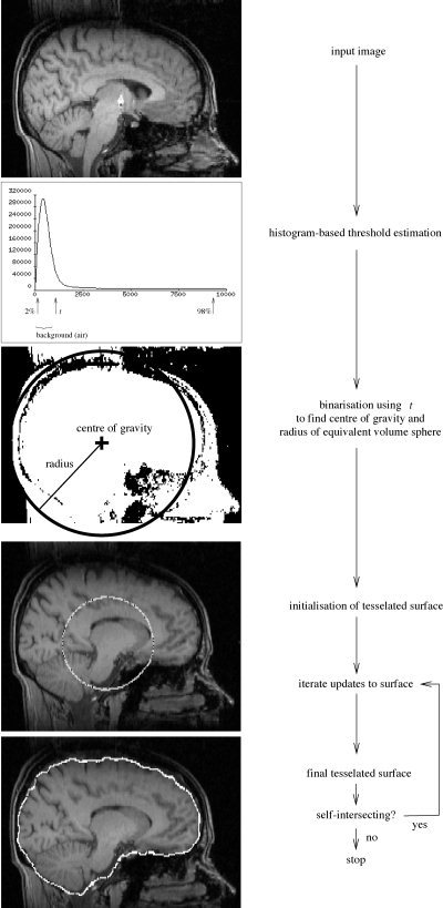
BET processing flowchart.

Estimation of basic image and brain parameters

The first processing that is carried out is the estimation of a few simple image parameters, to be used at various stages in subsequent analysis.

First, the robust image intensity minimum and maximum are found. Robust means the effective intensity extrema, calculated ignoring small numbers of voxels that have widely different values from the rest of the image. These are calculated by looking at the intensity histogram, and ignoring long low tails at each end. Thus, the intensity “minimum”, referred to as t ₂ is the intensity below which lies 2% of the cumulative histogram. Similarly, t ₉₈ is found. It is often important for the latter threshold to be calculated robustly, as it is quite common for brain images to contain a few high intensity “outlier” voxels; for example, the DC spike from image reconstruction, or arteries, which often appear much brighter than the rest of the image. Finally, a roughly chosen threshold is calculated that attempts to distinguish between brain matter and background (because bone appears dark in most MR images, “background” is taken to include bone). This t is simply set to lie 10% of the way between t ₂ and t ₉₈.

The brain/background threshold t is used to roughly estimate the position of the centre of gravity (COG) of the brain/head in the image. For all voxels with intensity greater than t, their intensity (“mass”) is used in a standard weighted sum of positions. Intensity values are upper limited at t ₉₈, so that extremely bright voxels do not skew the position of the COG.

Next, the mean “radius” of the brain/head in the image is estimated. There is no distinction made here between estimating the radius of the brain and the head, this estimate is very rough, and simply used to get an idea of the size of the brain in the image; it is used for initializing the brain surface model. All voxels with intensity greater than t are counted, and a radius is found, taking into account voxel volume, assuming a spherical brain. Finally, the median intensity of all points within a sphere of the estimated radius and centered on the estimated COG is found (t _m).

Surface model and initialization

The brain surface is modeled by a surface tessellation using connected triangles. The initial model is a tessellated sphere, generated by starting with an icosahedron and iteratively subdividing each triangle into four smaller triangles, while adjusting each vertex's distance from the centre to form as spherical a surface as possible. This is a common tessellation of the sphere. Each vertex has five or six neighbors, according to its position relative to the original icosahedron.

The spherical tessellated surface is initially centered on the COG, with its radius set to half of the estimated brain/head radius, i.e., intentionally small. Allowing the surface to grow to the optimal estimate gives better results in general than setting the initial size to be equal to (or larger than) the estimated brain size (see Fig. 7). An example final surface mesh can be seen in Figure 2.

Figure 7.

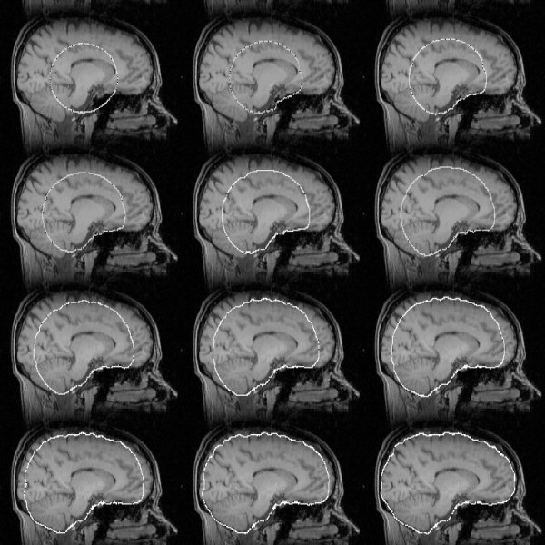
Example of surface model development as the main loop iterates. The dark points within the model outline are vertices.

Figure 2.

Three views of a typical surface mesh, shown for clarity with reduced mesh density.

The vertex positions are in real (floating point) space, i.e., not constrained to the voxel grid points. A major reason for this is that making incremental (small) adjustments to vertex positions would not be possible otherwise. Another obvious advantage is that the image does not need to be pre‐processed to be made up of cubic voxels.

Main iterated loop

Each vertex in the tessellated surface is updated by estimating where best that vertex should move to, to improve the surface. To find an optimal solution, each individual movement is small, with many (typically 1,000) iterations of each complete incremental surface update. In this context, “small movement” means small relative to the mean distance between neighboring vertices. Thus for each vertex, a small update movement vector u is calculated, using the following steps.

Local surface normal

First, the local unit vector surface normal n̂ is found. Each consecutive pair of [central vertex]−[neighbor A], [central vertex] − [neighbor B] vectors is taken and used to form the vector product (Fig. 3). The vector sum of these vectors is scaled to unit length to create n̂. By initially taking the sum of normal vectors before rescaling to unity, the sum is made relatively robust; the smaller a particular [central vertex]−[neighbor A]−[neighbor B] triangle is, the more poorly conditioned is the estimate of normal direction, but this normal will contribute less toward the sum of normals.

Figure 3.

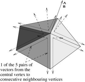
Creating local unit vector surface normal n̂ from all neighboring vertices.

Mean position of neighbors and difference vector

The next step is the calculation of the mean position of all vertices neighboring the vertex in question. This is used to find a difference vector s, the vector that takes the current vertex to the mean position of its neighbors. If this vector were minimized for all vertices (by positional updates), the surface would be forced to be smooth and all vertices would be equally spaced. Also, due to the fact that the surface is closed, the surface would gradually shrink.

Next, s is decomposed into orthogonal components, normal and tangential to the local surface;

(1)

and

(2)

For the 2D case, see Figure 4 (the extension to 3D is conceptually trivial). It is these two orthogonal vectors that form the basis for the three components of the vertex's movement vector u; these components will be combined, with relative weightings, to create an update vector u for every vertex in the surface. The three components of u are now described.

Figure 4.

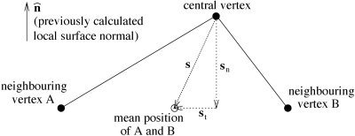
Decomposing the “perfect smoothness” vector s into components normal and tangential to the local surface.

Update component I: within‐surface vertex spacing

The simplest component of the update movement vector u is u ₁, the component that is tangential to the local surface. Its sole role is to keep all vertices in the surface equally spaced, moving them only within the surface. Thus, u ₁ is directly derived from s _t. To give simple stability to the update algorithm, u ₁ is not set equal to s _t, but to s _t/2; the current vertex is always tending toward the position of perfect within‐surface spacing (as are all others).

Update component 2: surface smoothness control

The remaining two components of u act parallel to the local surface normal. The first, u ₂, is derived directly from s _n, and acts to move the current vertex into line with its neighbors, thus increasing the smoothness of the surface. A simple rule here would be to take a constant fraction of s _n, in a manner equivalent to that of the previous component u ₂:

(3)

where f ₂ is the fractional update constant. Most other methods of surface modelling have taken this approach. A great improvement can be made, however, using a nonlinear function of s _n. The primary aim is to smooth high curvature in the surface model more heavily than low curvature. The reason for this is that although high curvature is undesirable in the brain surface model, forcing surface smoothing to an extent that gives stable and good results (in removing high curvature) weights too heavily against successful following of the low curvature parts of the surface. To keep the surface model sufficiently smooth for the overall algorithm to proceed stably, the surface is forced to be over‐smooth, causing the underestimation of curvature at certain parts, i.e., the “cutting of corners.” It has been found that this problem is not overcome by allowing f ₂ to vary during the series of iterations (this a natural improvement on a constant update fraction). Instead, a nonlinear function is used, starting by finding the local radius of curvature, r:

(4)

where l is the mean distance from vertex to neighboring vertex across the whole surface (Fig. 5). Now, a sigmoid function of r is applied, to find the update fraction:

(5)

where E and F control the scale and offset of the sigmoid. These are derived from a minimum and maximum radius of curvature; below the minimum r, heavy smoothing takes place (i.e., the surface deformation remains stable and highly curved features are smoothed), whereas above the maximum r, little surface smoothing is carried out (i.e., “long slow” curves are not over‐smoothed). The empirically optimized values for r _min and r _max are suited for typical geometries found in the human brain. Consideration of the tanh function suggests:

(6)

and

(7)

The resulting smoothness term (Fig. 6) gives much better results than a constant update fraction, both in ability to accurately model brain surface and in developmental stability during the many iterations.

Figure 5.

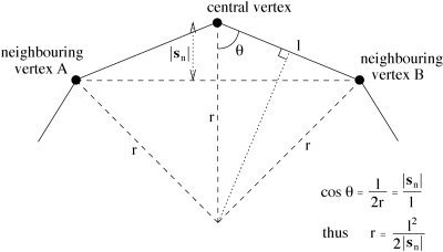
The relationship between local curvature r, vertex spacing l and the perpendicular component of the difference vector, |s _n|.

Figure 6.

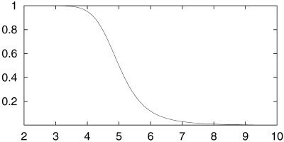
Smoothness update fraction vs. local radius of curvature, given r _max = 10 mm, r _min = 3.33 mm.

Update component 3: brain surface selection term

The final update component, u ₃, is also parallel to s _n, and is the term that actually interacts with the image, attempting to force the surface model to fit to the real brain surface. This term was originally inspired by the intensity term in [Dale et al., 1999]:

(8)

where the limits on d control a search amongst all image points x − d n along the surface normal pointing inward from the current vertex at x, and taking the product requires all intensities to be above a preset threshold. Thus whilst the surface lies within the brain, the resulting force is outward. As soon as the surface moves outside of the brain (e.g., into CSF or bone), one or more elements inside the product become zero and the product becomes zero. One limitation of this equation is that it can only push outward, thus the resulting surface is forced to be convex. A second limitation is the use of a single global intensity threshold I _thresh; ideally, this should be optimally varied over the image.

Thus, instead of the above equation, a much simpler core equation is used, embodying the same idea, but this is then extended to give greater robustness in a wider range of imaging sequences. First, along a line pointing inward from the current vertex, minimum and maximum intensities are found:

(9)

(10)

where d ₁ determines how far into the brain the minimum intensity is searched for, and d2 determines how far into the brain the maximum intensity is searched for. Typically, d ₁ = 20 mm and d ₂ = d ₁/2 (this ratio is empirically optimized, and reflects the relatively larger spatial reliability of the search for maximum intensity compared with the minimum). t _m, t ₂, and t are used to limit the effect of very dark or very bright voxels, and t is included in the maximum intensity search to limit the effect of very bright voxels. Note that the image positions where intensities are measured are in general between voxels as we are working in real (floating point) space, thus intensity interpolation needs to be used, interpolating between original voxel intensities. It was found that nearest neighbor interpolation gave better results than trilinear or higher order interpolations, presumably because it is more important to have access to the original (un‐interpolated, and therefore “unblurred”) intensities than that the values reflect optimal estimates of intensities at the correct point in space.

Now, I _max is used to create t _l, a locally appropriate intensity threshold that distinguishes between brain and background:

(11)

It lies a preset fraction of the way between the global robust low intensity threshold t ₂ and the local maximum intensity I _max, according to fractional constant b _t. This preset constant is the main parameter that BET can take as input. The default value of 0.5 has been found to give excellent results for most input images. For certain image intensity distributions it can be varied (in the range 0–1) to give optimal results. The necessity for this is rare, and for an MR sequence that requires changing b _t, one value normally works for all other images taken with the same sequence (the only other input parameter, and one that needs changing from the default even less often than b _t, for example, if there is very strong vertical intensity inhomogeneity, causes b _t to vary linearly with Z in the image, causing “tighter” brain estimation at the top of the brain, and “looser” estimation at the bottom, or vice versa). The update “fraction” is then given by:

(12)

with the factor of 2 causing a range in values of f ₃ of roughly −1 to 1. If I _min is lower than local threshold t _l, f ₃ is negative, causing the surface to move inward at the current point. If it is higher, then the surface moves outward.

The full update term is 0.05 f ₃ l. The update fraction is multiplied by a relative weighting constant, 0.05, and the mean inter‐vertex distance, l. The weighting constant sets the balance between the smoothness term and the intensity‐based term, it is found empirically, but because all terms in BET are invariant to changes in image voxel size, image contrast, mesh density, etc., this constant is not a “worked‐once” heuristic, it is always appropriate.

Final update equation

Thus the total update equation, for each vertex, is

(13)

Second pass: increased smoothing

One obvious constraint on the brain surface model is that it should not self‐intersect. Although it would be straightforward to force this constraint by adding an appropriate term to the update equation, in practice this check is extremely computationally expensive as it involves comparing the position of each vertex with that of every other at every iteration. As it stands, the algorithm already described rarely (around 5% of images) results in self‐intersection. A more feasible alternative is to run the standard algorithm and then perform a check for self‐intersection. If the surface is found to self‐intersect, the algorithm is re‐run, with much higher smoothness constraint (applied to concave parts of the surface only, it is not necessary for the convex parts) for the first 75% of the iterations; the smoothness weighting then linearly drops down to the original level over the remaining iterations. This results in preventing self‐intersection in almost all cases.

It has been suggested that there might be some value in re‐running BET on its own output. Although areas incorrectly “left in” after a first run might get removed on subsequent runs, it is our experience that this is not in general successful, presumably because the overall algorithm is not designed for this application.

Exterior skull surface estimation

A few applications require the estimation of the position of the skull in the image. A major example is in the measurement of brain atrophy [Smith et al., 2001]. Before brain change can be measured, two images of the brain, taken several months apart, have to be registered. Clearly this registration cannot allow rescaling, otherwise the overall atrophy will be underestimated. Because of possible changes in scanner geometry over time, however, it is necessary to hold the scale constant somehow. This can be achieved using the exterior skull surface, which is assumed to be relatively constant in size, as a scaling constraint in the registration.

In most MR images, the skull appears very dark. In T1‐weighted images the internal surface of the skull is largely indistinguishable from the cerebrospinal fluid (CSF), which is also dark. Thus the exterior surface is found. This also can be difficult to identify, even for trained clinical experts, but the algorithm is largely successful in its aim.

For each voxel lying on the brain surface found by BET, a line perpendicular to the local surface, pointing outward, is searched for the exterior surface of the skull, according to the following algorithm:

• Search outward from the brain surface, a distance of 30 mm, recording the maximum intensity and its position, and the minimum intensity.

• If the maximum intensity is not higher than t, assume that the skull is not measurable at this point, as there is no bright signal (scalp) on the far side of the skull. In this case do not proceed with the search at this point in the image. This would normally be due to signal loss at an image extreme, for example, at the top of the head.

• Find the point at greatest distance from brain surface d that has low intensity, according to maximization of the term d/30 − I(d)/(t ₉₈ − t ₂). The first part weighs in favor of increased distance, the second part weighs in favor of low intensity. The search is continued only out to the previously found position of maximum intensity. The resulting point should be close to the exterior surface of the skull.

• Finally, search outward from the previous point until the first maximum in intensity gradient is found. This is the estimated position of the exterior surface of the skull. This final stage gives a more well‐defined position for the surface, it does not depend on the weightings in the maximized term in the previous section, i.e., is more objective. For example, if the skull/scalp boundary is at all blurred, the final position will be less affected than the previous stage.

This method has been quite successful, even when fairly dark muscle lies between the skull and the brighter skin and fat. It is also mainly successful in ignoring the marrow within the bone, which sometimes is quite bright.

RESULTS

Example results

Figure 7 shows an example of surface model development as the main loop iterates, with a T1‐weighted image as input, finishing with the estimation shown in Figures 8 and 9. Figures 10, 11, 12 show example results on T2‐weighted, proton density, and echo planar imaging (EPI, widely used for FMRI) images. Figure 13 shows an example estimate of the exterior skull surface.

Figure 8.

Example brain surface generated by BET.

Figure 9.

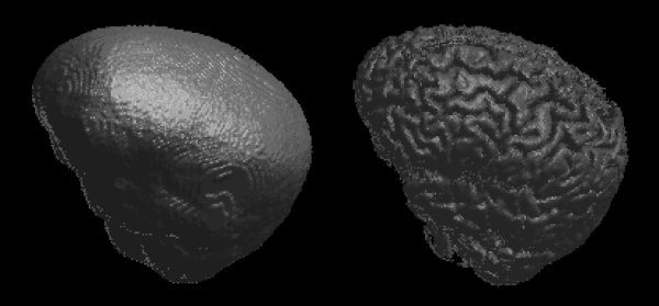
Example brain surface model (left) and resulting brain surface (right) generated by BET.

Figure 10.

Example brain surface from a T2‐weighted image.

Figure 11.

Example brain surface from a proton density image.

Figure 12.

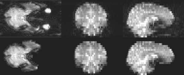
Example segmentation of an EPI image.

Figure 13.

Example exterior skull surface generated by BET.

Figure 14 shows the result of running BET on an EPI FMRI image that is heavily affected by ghosting. Clearly BET has worked well, both in removing the (outside‐brain) ghosting, and also in allowing registration (using FLIRT [Jenkinson and Smith, 2001]) to succeed.

Figure 14.

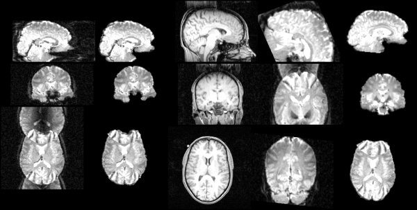
Left to right: the original FMRI image; BET output from the FMRI image; T1‐weighted structural image; (failed) registration without using BET; successful registration if BET is used.

Quantitative testing against “gold‐standard” and other methods

An extensive quantitative and objective test of BET has been carried out. We used 45 MR images, taken from 15 different scanners (mostly 1.5 T and some 3 T, from 6 different manufacturers), using a wide range of slice thicknesses (0.8–6 mm) and a variety of sequences (35 T1‐weighted, 6 T2‐weighted and 4 proton density). Hand segmentation of these images into brain/non‐brain1 was carried out. Thus, a simple binary mask was generated from each input image. Some slices from a sample hand segmentation are shown in the second column of Figure 15. BET and two other popular automated methods (“AFNI” and “BSE”) were tested against the hand segmentations.2

Figure 15.

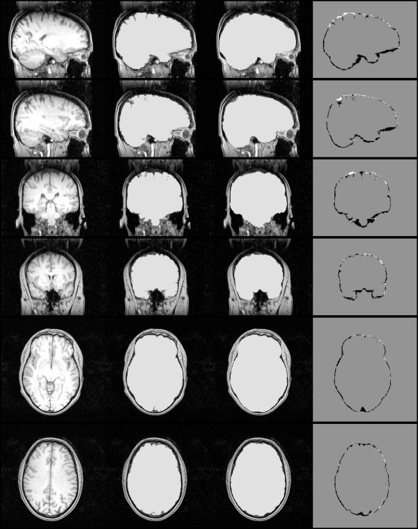
Left to right: example original whole‐head MR image; hand segmentation; fully automatic BET masking; hand mask minus BET mask.

The AFNI method [Cox,; Ward, 1999], though claiming to be fully automated, gave very poor results on most images (off the scale on Fig. 16), due to the failure of the initial histogram‐based choice of thresholds. Much better results were obtained by setting the initial thresholds using the simpler but more robust method described previously. The upper threshold was set to t ₉₈ and the lower threshold to 40% between t ₂ and t ₉₈. The refined method is referred to below as “AFNI*”.

Figure 16.

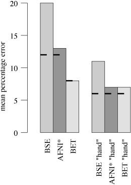
Mean % error over 45 MR images for three brain extraction methods, compared to hand segmentation; on the left are the results of testing the fully‐automated methods, on the right are the “hand‐optimized” results. The short bars show the results over only the 35 T1‐weighted images.

The results of the three methods were evaluated using a simple % error formulation of 0.5 × 100 × volume (total nonintersection)/volume (hand mask). The main results for the fully automated methods are shown on the left in Figure 16; the mean % error over the 45 images is shown for each method. The mean error is more meaningful than any robust measure (e.g., median) because outliers are considered relevant, the methods needs to be robust as well as accurate to be useful (though note that using median values instead gives the same relative results). The short bars show the results for the 35 T1‐weighted input images only. BET gives significantly better results than the other two methods. Some slices of a typical BET segmentation3 are displayed in the third column of Figure 15. The fourth column shows the hand mask minus the BET mask; in general BET is slightly overestimating the boundary (by approximately one voxel, except in the more complicated inferior regions), and smoothing across fine sulci.

It was also considered of interest to investigate the same test if initial controlling parameters were “hand‐optimized” (i.e., making the methods only “nearly fully optimized”). To carry this out in a reasonably objective manner, the primary controlling parameter for each method was varied over a wide range and the best result (comparing output with hand segmentation) was recorded. Fortunately, each method has one controlling parameter that has much greater effect on output than others, so the choice of which parameter to vary was simple.4 The range over which each method's principal controlling parameter was varied was chosen by hand such that the extremes were just having some useful effect in a few images. Each method was then run with the controlling parameter at nine different levels within the range specified. The results are shown on the right in Figure 16. The methods all improve to varying degrees. BET remains the best method, just beating AFNI*. The most important message from these results is that although BET is the most accurate and robust method in both tests, it is also the most successfully “fully automated.” Its results, when run fully‐automated, are nearly as good as those when it is “hand‐optimized.”

All the above comments on the quantitative results also hold when only the 35 T1‐weighted images are considered.

In theory it might be possible to “hand‐tune” a method once for a given MR pulse sequence, and the resulting parameters then work well for all images of all subjects acquired using this sequence. If this were the case, then possibly the results of AFNI* and BET could be viewed as similarly successful (assuming that our improvements to AFNI were implemented). This is, however, not the case. There was found to be significant variation in optimal controlling parameters for AFNI* (within‐sequence type).

Finally, note that results from a brain extraction algorithm may improve if the image is pre‐processed in certain ways, such as with an intensity inhomogeneity reduction algorithm. It is our experience, however, that the best intensity inhomogeneity reduction methods require brain extraction to have already been carried out.

CONCLUSION

An automated method for segmenting MR head images into brain and non‐brain has been developed. It is very robust and accurate and has been tested on thousands of data sets from a wide variety of scanners and taken with a wide variety of MR sequences. BET takes about 5–20 sec to run on a modern desktop computer and is freely available, as a standalone program that can be run from the command line or from a simple GUI, as part of FSL (FMRIB Software Library: http://www.fmrib.ox.ac.uk/fsl).

REFERENCES

- Atkins M, Mackiewich B (1998): Fully automatic segmentation of the brain in MRI. IEEE Trans Med Imaging 17: 98–107. [DOI] [PubMed] [Google Scholar]
- Bomans M, Höhne K‐H, Tiede U, Riemer M (1990): 3‐D Segmentation of MR images of the head for 3‐D display. IEEE Trans Med Imaging 9: 177–183. [DOI] [PubMed] [Google Scholar]
- Brummer M, Mersereau R, Eisner R, Lewine R (1993): Automatic detection of brain contours in MRI data sets. IEEE Trans Med Imaging 12: 153–166. [DOI] [PubMed] [Google Scholar]
- Cox R. AFNI software . Online: http://afni.nimh.nih.gov.
- Dale A, Fischl B, Sereno M (1999): Cortical surface‐based analysis I: segmentation and surface reconstruction. Neuroimage 9: 179–194. [DOI] [PubMed] [Google Scholar]
- Höhne K, Hanson W (1992): Interactive 3D segmentation of MRI and CT volumes using morphological operations. J Comp Assist Tomogr 16: 185–294. [DOI] [PubMed] [Google Scholar]
- Jenkinson M, Smith S (2001): A global optimization method for robust affine registration of brain images. Med Image Anal 5: 143–156. [DOI] [PubMed] [Google Scholar]
- Kass M, Witkin A, Terzopoulos D (1987): Snakes: active contour models. In: Proceedings of the 1st International Conference on Computer Vision, London, UK. p 259–268.
- Kelemen A, Székely G, Gerig G (1999): Elastic model‐based segmentation of 3D neuroradiological data sets. IEEE Trans Med Imaging 18: 828–839. [DOI] [PubMed] [Google Scholar]
- Kruggel F, von Cramen D (1999): Alignment of magnetic‐resonance brain datasets with the stereotactical coordinate system. Med Image Anal 3: 175–185. [DOI] [PubMed] [Google Scholar]
- Lemieux L, Hagemann G, Krakow K, Woermann FG (1999): Fast, accurate, and reproducible automatic segmentation of the brain in T1‐weighted volume MRI data. Magn Reson Med 42: 127–35. [DOI] [PubMed] [Google Scholar]
- Sandor S, Leahy R (1997): Surface‐based labeling of cortical anatomy using a deformable database. IEEE Trans Med Imaging 16: 41–54. [DOI] [PubMed] [Google Scholar]
- Smith S, De Stefano N, Jenkinson M, Matthews P (2001): Normalized accurate measurement of longitudinal brain change. J Comput Assist Tomogr 25: 466–475. [DOI] [PubMed] [Google Scholar]
- Smith S, Zhang Y, Jenkinson M, Chen J, Matthews P, Federico A, De Stefano N (2002): Accurate, robust and automated longitudinal and cross‐sectional brain change analysis. NeuroImage (in press). [DOI] [PubMed] [Google Scholar]
- Ward B (1999): Intracranial segmentation. Technical report. Medical College of Wisconsin Online at http://afni.nimh.nih.gov/afni/docpdf/3dIntracranial.pdf.
- Zhang Y, Brady M, Smith S (2001): Segmentation of brain MR images through a hidden Markov random field model and the expectation maximization algorithm. IEEE Trans Med Imaging 20: 45–57. [DOI] [PubMed] [Google Scholar]