Estimation of multiscale neurophysiologic parameters by electroencephalographic means

Abstract

It is shown that new model‐based electroencephalographic (EEG) methods can quantify neurophysiologic parameters that underlie EEG generation in ways that are complementary to and consistent with standard physiologic techniques. This is done by isolating parameter ranges that give good matches between model predictions and a variety of experimental EEG‐related phenomena simultaneously. Resulting constraints range from the submicrometer synaptic level to length scales of tens of centimeters, and from timescales of around 1 ms to 1 s or more, and are found to be consistent with independent physiologic and anatomic measures. In the process, a new method of obtaining model parameters from the data is developed, including a Monte Carlo implementation for use when not all input data are available. Overall, the approaches used are complementary to other methods, constraining allowable parameter ranges in different ways and leading to much tighter constraints overall. EEG methods often provide the most restrictive individual constraints. This approach opens a new, noninvasive window on quantitative brain analysis, with the ability to monitor temporal changes, and the potential to map spatial variations. Unlike traditional phenomenologic quantitative EEG measures, the methods proposed here are based explicitly on physiology and anatomy. Hum. Brain Mapping 23:53–72, 2004. © 2004 Wiley‐Liss, Inc.

INTRODUCTION

The central purpose of this study is to show how quantitative modeling of EEG generation enables estimation of underlying physiologic and anatomic parameters. It also demonstrates that the values obtained are consistent with, and complementary to, estimates obtained by a range of other means.

Correlations of electroencephalographic (EEG) measurements with brain function and physiology are widely used diagnostically [Niedermeyer and Lopes da Silva, 1999; Nunez, 1981, 1995] and are inferred to be connected closely to brain dynamics, information processing, cognition, and state of arousal [Coenen, 1995; Niedermeyer and Lopes da Silva, 1999; Nunez, 1995]. Despite this, it is only recently that links with underlying physiology and anatomy have been quantified systematically via explicit quantitative modeling of EEG generation, although a variety of EEG generation models have existed for three decades [Freeman, 1975, 1992; Jirsa and Haken, 1996; Lopes da Silva et al., 1974, 1976, 1980; Lumer et al., 1997; Nunez, 1974, 1981, 1995; Rennie et al., 1999, 2000, 2002; Robinson et al., 1997, 1998, 2001a, b, 2002, 2003a, c; Robinson, 2003; Wilson and Cowan, 1973; Wright and Liley, 1996; Zetterberg et al., 1978]. Moreover, the ability to systematically invert EEG data to estimate the parameters of underlying physiology has been realized only in the last year or two [Robinson et al., 2002; Rowe et al., 2003], although progress toward matching predictions to observations of various types was made in the above‐cited articles and elsewhere [Valdes et al., 1999; Wendling et al., 2000, 2001, 2002; Wright, 1999]. The aim of this study is to show that many neurophysiologic parameters can be constrained by model‐based EEG means, at length scales ranging from synaptic to whole‐brain levels and at time scales ranging from under 1 ms to 1 s or longer.

EEG phenomena result from cortical electrical activity aggregated over scales much larger than individual neurons but involving structures as small as synapses. A highly successful approach to understanding the dynamics of the 10¹¹ neurons of the brain is via models that average over microscopic neural structure to obtain continuum descriptions on scales of millimeters to the whole brain, incorporating realistic features such as separate excitatory and inhibitory neural populations (pyramidal cells and inter‐neurons), nonlinear neural responses, synaptic, dendritic, cell body, and axonal dynamics, and corticothalamic feedback [Freeman, 1975, 1992; Jirsa and Haken, 1996; Lopes da Silva et al., 1974, 1976; Nunez, 1981, 1995; Rennie et al., 1999, 2000, 2002; Robinson et al., 1997, 1998, 2001a, b, 2002, 2003a, c; Wilson and Cowan, 1973; Wright and Liley, 1996]. This style of modeling complements the considerable body of work dealing with single neurons and neural networks [e.g., Dayan and Abbott, 2001; Koch, 1999].

A recent physiologically based continuum model of corticothalamic dynamics has been found to reproduce many features of normal EEGs including time series, spectra, evoked response potentials, coherence, correlations, arousal changes, and seizure dynamics [O'Connor et al., 2002; O'Connor and Robinson, 2003a, b; Rennie et al., 1999, 2000, 2002; Robinson et al., 1997, 1998, 2001b, 2002; Robinson, 2003]. Agreement of model predictions with a variety of data is found for model parameters that lie in physiologically realistic ranges. Moreover, because the model has sufficient parameters to describe salient features of the brain, but not so many as to be ill conditioned, unconstrained fitting of predictions to some types of data is possible (i.e., adjustment of model parameters to get the best possible match). Such fitting also yields outcomes that lie in physiologically realistic ranges [Robinson et al., 2002; Rowe et al., 2003].

A key feature of the above model is that it involves, and hence probes (i.e., is sensitive to), parameters that are of functional significance to EEG generation and to other aspects of brain function. Synaptic parameters such as time constants and strengths of neurotransmitter release and reuptake are probed, as are time constants for signal propagation along dendrites. Inferences can also be made about the parameters of the nonlinear integrate‐and‐fire response at the cell body, and about speeds, ranges, and time delays of subsequent axonal propagation, both within the cortex and on paths involving the thalamus. Finally, it is possible to estimate quantities that parametrize volume conduction in tissues overlying the cortex, which affect EEG measurements. Each of these parameters is constrained independently by physiologic and anatomic measurements or, in a few cases, by other types of modeling. A key point in our modeling is that we strike a balance between our model having too few parameters to be realistic and too many for the data to be able to robustly constrain them, and thus avoid the problem of free parameters that can be adjusted at will. Our model has no free parameters, although some are only relatively poorly known from independent physiologic studies to date.

We focus on parameters that are pertinent to and accessible via current continuum modeling. We show that these can be estimated by EEG means, and yield values that are consistent with other measures. We also demonstrate that the constraints provided by EEG phenomena are often complementary to those obtained by other means, leading to much tighter constraints overall. Finally, we show how the approach used here yields a noninvasive probe of multiscale neurophysiology and anatomy that can be used to map these parameters. To keep the scope of the article manageable, we concentrate on alert, wakeful, normal adults, except where particular insights from other cases are essential.

MATERIALS AND METHODS

We first outline our model and explain its key parameters. (Note: the mathematical formulation is given here for completeness but understanding the details is not essential to follow the remainder of this article.) Generalizations of the model presented here are possible, and directions for these are indicated in places but they are not pursued because they are not relevant to the comparisons made within this article. In latter subsections we discuss how comparisons between model predictions and data drawn from the literature can be used to constrain these parameters. We stress that it is not our purpose to revisit the full derivation and justification of the model, nor all the details of its application to specific phenomena; these are found in the references cited. Rather, we explore the implications for inferring neurophysiology if the model is accepted provisionally, specifically, the extent to which model‐based inferences are consistent with and complement independent measures.

The Model

Our model incorporates key anatomic connectivities within the cortex, within the thalamus, and between these structures, as shown schematically in Figure 1. These connectivities include projections from the cortex to the thalamic reticular nucleus (by which we also refer to the perigeniculate nucleus, which serves analogous functions [Sherman and Guillery, 2001]), which inhibits thalamic relay nuclei via GABAergic projections. The relay nuclei transfer external stimuli to the cortex and reticular nucleus, along with corticothalamic feedback via glutamatergic projections of cortical activity to them, and their influences are excitatory, also mainly via glutamatergic projections. The cortex itself is treated as a continuum containing populations of interacting excitatory and inhibitory neurons and is approximated as two‐dimensional (2‐D) owing to its relative thinness.

Figure 1.

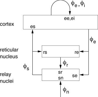
Schematic of corticothalamic interactions, showing the connectivities and locations ab of the gains G _ab for impulses from neurons b incident on neurons of type a. The cortex and the reticular and relay nuclei of the thalamus are shown as rectangles, along with the main neural projections between them (the latter are indicated by arrows, labeled with the type of activity that projects). External activity is indicated by ϕ_n.

In the continuum approximation, each actual quantity at a given point is replaced by the average of the same quantity over a region, a few tenths of a millimeter wide, surrounding that point. This corresponds to a smoothing of local quantities over scales shorter than this but does not imply that all information about shorter‐scale structures is discarded; on the contrary, it is retained in spatially smoothed form.

In the cortex the mean firing rates (i.e., pulse densities) Q _a of excitatory (a = e) and inhibitory (a = i) neurons are related to the corresponding cell body potentials V _a, relative to resting, by Q _a(r, t) = S[V _a(r, t)], where S is a smooth sigmoidal function that increases from 0 to Q _max as V _a increases from −∞ to ∞. We model S by the form

(1)

where Q _max is the maximum attainable firing rate, θ is the mean firing threshold, and σ′ /π is the standard deviation of the threshold distribution in the neural population. This relationship could be generalized to allow a different functional form for each neural population (at the cost of introducing additional parameters), but we do not do so here, so the parameters Q _max, θ, and σ′ are interpreted as effective values, averaged over all populations.

Signals arriving at neurons of type a stimulate neurotransmitter release at synapses. This is followed by propagation of voltage changes along dendrites, with cable properties that tend to spread out the temporal profile of the signals (a form of low‐pass filtering). The total cell body potential V _a can thus be written as [Robinson et al., 1997, 2001a, b, 2002, 2003a, c]

(2)

where the subscript b on the components V _ab distinguishes the different combinations of afferent neural type and synaptic receptor. For present purposes, we take a weighted average over the receptor time constants to yield effective values that will change when and if different receptors dominate the dynamics in different brain states. (This approximation can also be avoided at the cost of introducing additional parameters.) We can then write [Robinson et al., 2002, 2003a, c]

(3)

(4)

In these equations, the quantity D_a encapsulates the overall time constants, 1/β and 1/α of the rise and fall, respectively, of the response at the cell body, after allowing for receptor dynamics and dendritic propagation. Effectively, 1/β is the longer of the receptor and dendritic rise times, and 1/α is the longer of the corresponding fall times. The use of a single form of D_a corresponds to the approximation that the mean dendritic dynamics can be described by a single pair of time constants. On the right of equation (3), V _ab(r,t) has been replaced by N _ab s _bϕ_b(r t − τ_ab) where N _ab is the mean number of synapses on neurons a from neurons of type b, s _ab is the mean time‐integrated strength of soma response per incoming spike, and ϕ_b(r,t − τ_ab) is the mean spike arrival rate from neurons b, allowing for a time delay τ_ab due to anatomic separations. The quantities a and b correspond to the excitatory (e), inhibitory (i), reticular thalamic (r), and specific relay (s) populations, and to external stimuli (n). The only nonzero values of τ_ab in our model are τ_es = τ_se = τ_re = t ₀/2, which correspond to corticothalamic and thalamocortical propagation times. The time t ₀ can be related to the characteristic loop length R and mean axonal velocity V by t ₀ = R/V.

Each part of the corticothalamic system gives rise to neural pulses, whose values averaged over short scales form a field ϕ_a(r,t) in our model that propagates at a velocity v _a. To a good approximation, ϕ_a obeys a damped wave equation whose source of pulses is:

(5)

(6)

[Robinson et al., 1997, 2001a, b, 2002, 2003a, c], where isotropy has been assumed, r _a is the mean range of axons of type a, and γ_a = v _a/r _a is the temporal damping rate of pulses in axons a. In our model, only the axons of excitatory cortical neurons e are long enough to yield significant propagation effects; in the other cases, γ_a is so large that the solution of equations (5) and (6) can be approximated by ϕ_a(r,t) = S[V _a(r,t)], which we term the local activity approximation.

Under the local activity approximation, equations (1) to (6) can be solved numerically to predict the response to specified incoming signals ϕ_n in terms of the 16 quantities t ₀, α, β, γ_e, r _e, Q _max, θ, σ′, and N _ab s _ab (this product is also termed ν_ab below, and we treat eight of these as nonzero and independent on the assumption of random cortical connectivity, which implies N _ib = N _eb for all b). If the variables ϕ_a/Q _max, ν_ab/Q _maxσ′, t/t ₀, V _a/σ′, and r/r _e are used in place of the dimensional forms, one finds that the solutions depend only on these dimensionless forms, lowering the essential dimensionality of parameter space to 11. This reflects scaling properties under variation of the maximum firing rate, strength of interconnection, time scale, voltage scale, and length scale, respectively.

Steady States and Linear Transfer Functions

If the time and space derivatives in equations (1) to (6) are set to zero, we obtain a nonlinear equation for the uniform steady states of brain activity. In terms of the steady‐state value ϕ${}_{\mathit{\text{e}}}^{\text{(0)}}$ of ϕ_e, this is

(7)

Investigation of this equation shows that it has stable steady‐state solutions corresponding to low and very high mean firing rates, the former of which we have identified with normal states of brain activity [Robinson et al., 1997, 1998].

In many cases we can approximate the brain's activity as being perturbed relative to a steady state, and adopt a linear approximation. This enables some important predictions to be obtained analytically. In the regime that is linear in the ϕ_a, perturbations relative to steady‐state values ϕ${}_{\mathit{\text{a}}}^{\text{(0)}}$ and V ${}_{\mathit{\text{a}}}^{\text{(}\mathit{\text{0}}\text{)}}$ approximately obey the damped wave equation [Robinson et al., 1997, 2001b, 2002]

(8)

where we henceforth use the symbols ϕ_a and V _a to denote linear perturbations of these quantities relative to their steady‐state values, unless otherwise indicated, and ρ_a = dS(V_a)/dV_a evaluated at the steady state value of V _a. For the form given by equation (1), one finds

(9)

Operation with D_a on both sides of equation (7), with use of equation (3), then yields

(10)

where the gain G _ab = ρ_aν_ab = ρ_a N _ab s _ab is the response in neurons a due to unit input from neurons b, i.e., the number of additional pulses out for each additional pulse in.

If we Fourier transform equation (10) in space and time, we find transfer functions that enable us to express the firing rates in terms of the external signal ϕ_n. In particular, we find

(11)

(12)

(13)

(14)

(15)

(16)

(17)

where k and ω are the wave vector and angular frequency, respectively. (The wavelength is 2π/k and the usual frequency in Hz is ω/2π.) Note that, of the eight nonzero G _ab in the model (allowing for the fact that G _ib = G _eb for all b if cortical neurons are interconnected randomly [Robinson et al., 1997; Wright and Liley, 1996]), only G _ee, G _ei, G _esn = G _es G _sn and the combinations in equations (14) to (16) appear in the linear limit. This gives a total of 11 parameters, of which G _esn only affects normalization of ϕ_e. Of these 11, only 8 are essential because time, distance, and firing rate can all be rescaled as before (the possibility of voltage and coupling‐strength rescalings have been absorbed into the G _ab, which are already dimensionless).

The importance of the transfer function T _en of linear perturbations arises because scalp potentials are generated primarily by excitatory (mainly pyramidal) neurons, owing to their greater size and degree of alignment compared to other types [Nunez, 1995; O'Connor and Robinson, 2003a, b; Rennie et al., 2002]. For any given geometry the scalp potential is proportional to the cortical potential, which is itself proportional to the mean cellular membrane currents, which are in turn proportional to the firing rates ϕ_e,i, which prove to be approximately proportional to one another in our model. Hence, apart from a (dimensional) constant of proportionality, and the effects of volume condition in the skull, scalp, and cerebrospinal fluid, scalp EEG signals correspond closely to ϕ_e.

Volume conduction in tissues between the cortex and scalp electrodes has the effect of attenuating signals with short spatial scales. This effect can be approximately taken into account by including a spatial filter function, such that signals are attenuated at wave numbers k > k ₀, where k ₀ is the characteristic low‐pass wave number. The results are not very sensitive to the precise form of the filter function [O'Connor et al., 2002; Robinson et al., 2001b].

Linear Model Predictions

For linear perturbations relative to the steady state, the transfer function, equation (11), forms the basis for a range of predictions, because ϕ_e(k,ω) = |T _en(k,ω)ϕ_n(k,ω)|. First, the combined frequency‐wavenumber spectrum of the EEG is

(18)

The usual frequency spectrum can be written as

(19)

which can be evaluated analytically for some forms of ϕ_n, including white noise [Robinson et al., 1997]. If we make the assumption that under conditions of spontaneous EEG the field of external stimuli ϕ_n(k,ω) is so complex that it can be approximated by spatiotemporal white noise, this gives |ϕ_n(k,ω)|² = constant. In the white noise case

(20)

where 〈ϕ${}_{\mathit{\text{n}}}^{\text{2}}$〉 is the mean‐square noise level, Arg denotes the complex argument and Im is the imaginary part. Figure 2 shows a comparison between this formula and EEG spectral data from a normal subject, demonstrating the close match achieved [Robinson et al., 2003a]. Further analysis of this expression shows that the alpha rhythm has a period T _α that depends on propagation and dendritic delays in the corticothalamic loop [Robinson et al., 2001a, b, 2002], with

(21)

Similar analysis shows that sleep spindles have a frequency f _σ related to the dendritic time constants, via

(22)

[Robinson et al., 2002].

Figure 2.

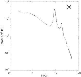
Model predictions vs. data, showing predicted EEG spectrum for a normal adult in the relaxed eyes‐closed state (dotted curve) vs. data (solid) [Robinson et al., 2003a].

One key point is that our model implies that the alpha, beta, and other rhythms are generated as resonances in corticothalamic and intrathalamic loops. This contrasts with pacemaker mechanisms that simply postulate ad hoc a group of pacemaker cells that produce each frequency seen. It also contrasts with theories based on purely cortical resonant modes which do not account for known aspects of thalamic involvement in the generation of brain rhythms [e.g., Steriade et al., 1997]. Detailed discussions of the relative strengths and weaknesses of these theories are found in Robinson et al. [2001a, 2003c]. Their conclusion was that, overall, the corticothalamic model gives the best match to data.

The wavenumber spectrum is

(23)

an expression that has been compared successfully with a variety of data on the wavenumber content of EEGs and electrocorticograms (ECoGs) [O'Connor et al., 2002; O'Connor and Robinson, 2003a, b].

Time series of EEGs can be calculated by inverse Fourier transforming ϕ_e(k,ω). This gives

(24)

In the case of spontaneous EEG, ϕ_n is approximated by random‐phase white noise in equation (24), whereas it is replaced by the (constant) Fourier transform of a δ function for an impulsive stimulus to calculate event‐related potentials (ERPs). Figure 3 shows the close agreement between theory and data from scalp recordings of an auditory ERP, evoked in response to a background tone under an oddball paradigm [Rennie et al., 2002; Robinson et al., 2003a]. Steady‐state evoked potentials (SSEPs, the responses to sinusoidal stimuli) ϕ_e(r,ω) are calculated by omitting the Fourier transform over ω in equation (24) and assuming a monochromatic input ϕ_n with spatial structure appropriate to the stimulus.

Figure 3.

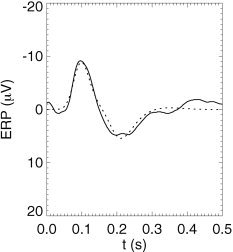
Model predictions vs. data, showing predicted background auditory ERP (dotted) vs. data (solid) [Robinson et al., 2003a].

The spatiotemporal correlation function is given by the Fourier transform of the frequency–wavenumber spectrum, with

(25)

(26)

being the unnormalized correlation function of signals at points separated by a displacement R and a time interval T, with the angle brackets indicating an average over r and t. Likewise, the temporal correlation function is the temporal Fourier transform of P(ω), and the spatial one is the spatial Fourier transform of P(k). One can also write the cross spectrum

(27)

(28)

where the angle brackets indicate an average over r.

The coherence function γ² can be obtained from the above results, with

(29)

where homogeneity has been assumed. If the system is also isotropic, the results in equations (25) to (29) depend only on the magnitude of R, rather than on the vector displacement R. Obviously, these assumptions are only first approximations, but they are sufficient for initial comparisons of theory with EEG and ECoG data, which show good agreement as functions of distance and frequency [Robinson, 2003].

If system boundary conditions are introduced, they impose a discrete mode structure on the fields and the integrals over k in the above results must be replaced by sums over modes [Robinson et al., 2001a, 2003c]; we will not show this explicitly here because it merely serves to complicate the notation. Where appropriate, this feature was incorporated in the original articles from which the results discussed below are drawn.

Nonlinear Model Predictions

In the nonlinear regime, fewer analytic results can be obtained. One can find limits on the stability of the brain, which lead to corresponding limits on the model parameters [Robinson et al., 2002]. Of particular relevance here, the existence of steady states with comparable values of ϕ${}_{\mathit{\text{e}}}^{\text{(0)}}$, ϕ${}_{\mathit{\text{s}}}^{\text{(0)}}$, ϕ${}_{\mathit{\text{r}}}^{\text{(0)}}$, and ϕ${}_{\mathit{\text{n}}}^{\text{(0)}}$ is possible only if the conditions

(30)

(31)

(32)

where ϕ_c is the assumed common characteristic value of the various ϕ${}_{\mathit{\text{a}}}^{\text{(0)}}$, A = 1/e if all the firing rates are equal, and A ≃ 1 if one dominates. If the steady‐state values are approximately proportional to one another in the range of interest, it is possible to show further that

(33)

for a = e, s, r, where

(34)

is the resting firing rate in the complete absence of inputs. In the waking state, the net inputs are believed to be excitatory overall (Steriade et al., 1997), leading to the additional results

(35)

(36)

for a, b = e, s, r, where equation (36) follows from equation (35). These results imply A ≤ 1 in equations (30) to (32).

Model‐Based Parameter Constraints

In previous work, we have compared a range of model predictions with data, drawn from the literature on spatial and temporal aspects of EEGs, ERPs, coherence measures, and correlations [O'Connor et al., 2002; O'Connor and Robinson, 2003a, b; Rennie et al., 2000, 2002; Robinson et al., 2001b, 2002, 2003a, c; Robinson, 2003; Rowe et al., 2003]. The agreement was excellent with a wide range of data, implying that this single model has the ability to reproduce a range of phenomena. The success of these predictions encourages us to argue that the parameter values that yield optimal matches with data are good estimates of the actual values in the brain. This enables us to constrain these parameters, both via fits and by means of other insights obtained from the model, and establishes the importance of the model parameters themselves, some of which are not measured commonly by physiologists. Specific model‐based constraints are outlined here, and the actual values of these constraints are detailed in the results.

The dynamics of brain activity, as opposed to steady‐state levels, show clear nonlinear features only a few percent of the time [Breakspear, 2002; Stam et al., 1999]. If the brain's voltage perturbations are in the linear regime, this constrains perturbations of V _a relative to steady states to be smaller than σ′ in equation (1). In a similar vein, both normal and idling levels of activity are much smaller than Q _max, which constrains θ /σ′ in equation (1) to be large enough that exp(−θ /σ′) << 1. Likewise, the fact that EEG potentials and neural firing rates during seizures can be an order of magnitude or more greater than are those during normal states implies that normal firing rates satisfy ϕ${}_{\mathit{\text{a}}}^{\text{(0)}}$/Q _max ≲ 0.1. On the other hand, the nonlinear interaction seen between slow and fast waves in slow‐wave sleep [Niedermeyer and Lopes da Silva, 1999; Steriade, 2000, 2001; Steriade et al., 1997, 2001; Timofeev et al., 1996] implies that slow waves involve perturbation potentials that are ≳ σ′, with minimums well below (hyperpolarized relative to) the firing threshold; coma presumably exists entirely in the relatively hyperpolarized state. Similarly, the detection of nonlinear interactions in a few percent of cases [Breakspear, 2002; Stam et al., 1999] implies that membrane potential amplitudes of alpha waves can approach σ′ in magnitude in at least some individuals.

Nonlinear least‐squares fits of theoretical frequency spectra to scalp EEG data yield estimates of the linear parameters of the model, which prove to be highly robust and reproducible: t ₀ is tightly constrained by the value of the alpha period T _α, given by equation (22). This relationship also constrains α and β, which are restricted further by the need to match the overall shape of the spectrum because they determine the location of a knee near 15 Hz where the spectrum begins to fall off more steeply at higher frequencies. The other linear parameters are constrained in more complex ways by finer details of the spectrum, including that the 1/f nature of the low‐frequency part of the spectrum implies that the system is near marginal stability [Robinson et al., 1997, 2001b]. As noted above, the model also predicts frequencies of specific rhythms and these constrain the various temporal quantities appearing in equations (21) and (22). Overall, such fits typically yield estimates of α, β, γ_e, t ₀, G _ee, G _ei, G _ese, G _esre, G _srs, and k ₀ [Rowe et al., 2003].

If, in addition to the above linear fit parameters, the mean firing rates are known, the following new analysis yields the remaining G _ab and the nonlinear parameters ν_ab. The mean rates are not likely to be available for individuals but may be estimated for groups. If they are only approximately known, Monte Carlo inversion (see below) can be used to obtain probability distributions of the parameter values.

If firing rates are low compared to Q _max, the sigmoid given by equation (1) can be approximated by

(37)

If the mean firing rates ϕ${}_{\mathit{\text{a}}}^{\text{(0)}}$ and linear fit parameters mentioned above are known in the state of interest, they enable inversion of the nonlinear model. Specifically, if the time and space derivatives in equations (1) to (6) are set to zero, equation (37) yields

(38)

(39)

(40)

where ϕ˜_a = ϕ${}_{\mathit{\text{a}}}^{\text{(0)}}$/ϕ₀. Solution of the above equations yields

(41)

(42)

(43)

(44)

(45)

(46)

The parameters ν_ab of the nonlinear model can then be obtained from ν_ab ≈ G _abσ′/ϕ${}_{\mathit{\text{a}}}^{\text{(0)}}$ in the low −ϕ${}_{\mathit{\text{a}}}^{\text{(0)}}$ limit. Once the linear fit parameters have been determined, the other G _ab depend only on ratios of the ϕ˜_a, apart from slowly varying logarithmic terms. If the ϕ${}_{\mathit{\text{a}}}^{\text{(0)}}$ are known only approximately, probability distributions of the nonlinear parameters can be obtained by Monte Carlo means by throwing random values of the ϕ${}_{\mathit{\text{a}}}^{\text{(0)}}$ within any known constraints, inverting via the above equations, and then binning the resulting values.

Fits to human and animal EEG and ECoG wavenumber spectra yield parameters similar to those obtained via frequency spectrum fits, but give more direct information on spatial parameters. For example, features are seen in wavenumber spectra at wavenumbers near 1/r _e and 1/r _m, respectively, where r _m is the range of recurrent intermediate‐range excitatory axons incorporated in a refinement of our model [O'Connor and Robinson, 2003a, b; Rennie et al., 2002]. These fits also yield information on the relative contributions of excitatory, intermediate‐range recurrent excitatory, and inhibitory neurons to the EEG, confirming the dominant contribution of the former [O'Connor and Robinson, 2003a, b].

Matching model predictions with observed evoked potentials also constrains all the parameters, with particular constraints on t ₀ and some of the corticothalamic gains, with the values obtained being consistent with those from EEG spectral fits [Rennie et al., 2002].

Analysis of the distance dependence of EEG and ECoG coherence constrains all the parameters, yielding particularly direct information on the ranges r _e and r _m. It also constrains the values of k ₀ that are consistent with data [Robinson, 2003]. The dependence of coherence on frequency also provides a constraint on t ₀ [Robinson, 2003].

Other Parameter Constraints

The other types of parameter constraints used in this work derive primarily from direct physiologic and anatomic measurements of the parameters in Table I and other quantities in our model, including t ₀, r _e, v, R, V, N _ab, s _ab, ϕ_a, Q _max, θ, and σ′. These are drawn directly from the literature, and we discuss the resulting bounds on parameters in the results.

Table I.

Brain parameters for normal adults in the alert, eyes‐open state

Quantity	Symbol	Prior range	Range	Estimate	Unit
Corticocortical e axon
Rangea, b	r e	50–200	89 ± 9	86	mm
Axonal velocity	υe	6–11	9.8 ± 1.2	10	m/s
Cortical damping ratea, b	γe = υe/r e	30–220	116 ± 4	116	s−1
Corticothalamic
Axonal velocity	V	4–11	4.5 ± 0.5	4.2	m/s
Loop distance	R	100–400	360 ± 40	360	mm
Loop delaya, b	t 0 = R/V	9–100	85 ± 1	85	ms
Synaptodendritic
Decay timea, b	1/α	5–200	12 ± 2	12	ms
Rise timea, b	1/β	0.4–60	1.3 ± 0.3	1.3	ms
Maximum firing ratea	Q max	100–1,000	220–500	340	s−1
Firing thresholda	θ	10–25	10–17	13	mV
Threshold spreada	σ′	2–6	3.8 ± 0.2	3.8	mV
Threshold ratio	θ/σ′	1.7–12	3.4 ± 0.9	3.4	—
Firing rate
e Neurons	ϕ${}_{\mathit{\text{e}}}^{\text{(0)}}$	16 ± 2	16 ± 2	16	s−1
s Neurons	ϕ${}_{\mathit{\text{s}}}^{\text{(0)}}$	16 ± 7	16 ± 7	16	s−1
r Neurons	ϕ${}_{\mathit{\text{r}}}^{\text{(0)}}$	24 ± 5	24 ± 5	24	s−1
n Neurons	ϕ${}_{\mathit{\text{n}}}^{\text{(0)}}$	16 ± 4	16 ± 4	16	s−1
Resting firing rate	ϕ0	4–18	7–18	11	s−1
Sigmoid slope
For e neurons	ρe	1–10	3.5–5.0	4.2	(mV s)−1
For s neurons	ρs	1–10	2.0–6.7	4.2	(mV s)−1
For r neurons	ρr	1–10	5.0–7.6	6.3	(mV s)−1
Afferent synapses
Per e neuron	N e = N ee + N ei + N es	(4–40) × 103	(4–40) × 103	1.2 × 104	—
Per s neuron	N s = N se + N sr + N sn	1,000–8,000	1,000–8,000	2,100	—
Per r neuron	N r = N re + N rs	1,000–8,000	1,000–8,000	3,400	—
e Synapses/e neuron	N ee = (0.75–0.85)N e	(3–34) × 103	(3–34) × 103	104	—
i Synapses/e neuron	N ei = (0.1–0.15)N e	400–6,000	400–6,000	1,600	—
s Synapses/e neuron	N es = (0.05–0.1)N e	200–4,000	200–4,000	800	—
e Synapses/s neuron	N se = (0.3–0.6)N s	300–4,800	300–4,800	1,100	—
r Synapses/s neuron	N sr = (0.2–0.4)N s	200–3,200	200–3,200	550	—
n Synapses/s neuron	N sn = (0.1–0.5)N s	100–4,000	100–4,000	450	—
e Synapses/r neuron	N re = (0.7–0.8)N r	700–6,400	700–6,400	2,700	—
s Synapses/r neuron	N rs = (0.2–0.3)N r	200–2,400	200–2,400	700	—
Synapse strength
e Synapse on e neuron	s ee	<10	0.03–0.7	0.15	μV s
i Synapse on e neuron	−s ei	<10	0.3–6	1.3	μV s
s Synapse on e neuron	s es	<10	0.05–5	0.5	μV s
e Synapse on s neuron	s se	<10	0.04–6	0.5	μV s
r Synapse on s neuron	−s sr	<10	0.06–10	0.8	μV s
n Synapse on s neuron	s sn	<10	0.03–5	0.4	μV s
e Synapse on r neuron	s re	<10	0.004–0.5	0.07	μV s
s Synapse on r neuron	s rs	<10	0.003–0.3	0.05	μV s
Synaptic producta
ee	νee = N ee s ee	0.3–340	1.6 ± 0.4	1.60	mV s
ei	−νei = −N ei s ei	0.04–60	1.9 ± 0.5	1.90	mV s
es	νes = N es s es	0.02–40	0.2–1.0	0.39	mV s
se	νse = N se s se	0.03–48	0.2–2.0	0.60	mV s
sr	−νsr = −N sr s sr	0.02–32	0.2–2.8	0.45	mV s
sn	νsn = N sn s sn	0.01–40	0.1–0.5	0.15	mV s
re	νre = N re s re	0.07–64	0.03–0.3	0.15	mV s
rs	νrs = N rs s rs	0.02–24	0.007–0.06	0.03	mV s
Gain
ee b	G ee	3–3,400	6.8 ± 0.2	6.8	—
ei b	−G ei	0.4–600	8.1 ± 0.2	8.1	—
es	G es	0.2–400	0.9–3.3	1.7	—
se	G se	0.3–480	1.1–3.8	2.5	—
sr	−G sr	0.2–320	1.2–5.5	1.9	—
sn	G sn	0.7–1.0	0.7–1.0	0.8	—
re	G re	0.7–640	0.25–1.3	1.0	—
rs	G rs	0.2–240	0.06–0.28	0.19	—
Positive CT loopb	G ese = G es G se	6 × 10−4–2,000	4.2 ± 0.2	4.2	—
Negative CT loopb	−G esre = −G es G sr G re	3 × 10−5–8 × 104	3.1 ± 0.1	3.1	—
Intrathalamic loop	−G srs = −G sr G rs	6 × 10−4–800	0.37 ± 0.05	0.37	—
Input path	G esn = G es G sn	0.4–400	0.6–3.3	1.4	—
Spatial low‐pass wavenumber	k 0	—	29 ± 9	29	m−1
Spatial low‐pass wavenumber × r e a, b	k 0 r e	—	2.5 ± 0.5	2.5	—

The first column gives a brief description of the parameter, with its symbol listed in the second. The third column gives the range currently obtainable without imposing model‐based constraints, while the fourth gives the range obtained here. The fifth column gives a self‐consistent nominal set of parameters. Units of each quantity given in the final column. Only quantities discussed in the present work are listed and concentrate on mean values; individuals will scatter within and around the ranges quoted.

^aParameters required for the nonlinear version of the model.

^bParameters required for the linear version of the model.

CT, corticothalamic.

The final constraint discussed here is obtained from independent modeling of some of the elementary processes involved in the EEG, especially from analysis of the effects of volume conduction, which enables values of k ₀ to be estimated from the conductance properties of the cerebrospinal fluid, skull, and scalp [Nunez, 1981, 1995; Srinivasan et al., 1998].

Combination of Constraints

Many of the above constraints are indirect or complement others, rather than simply measuring the same quantity by another means. As detailed in the next sections, we find that the power of these constraints is multiplied by considering groups of variables together, as well as singly. In two‐variable (or more) parameter spaces, constraints often intersect to yield only small zones in which the parameters are consistent with all the constraints simultaneously.

RESULTS

In this section, we work systematically through constraints on various parameters, mostly taken singly or pairwise, to obtain the most restrictive constraint set. The analysis is carried out for the most common human state of arousal, which is the alert waking state in normal adults, except where noted otherwise. We also concentrate on constraints on mean values, noting that individuals' parameters will scatter somewhat around these means. Finally, we present a self‐consistent set of nominal values that satisfies all constraints simultaneously, and which will be of particular use in future work where specific illustrative values are needed.

Corticocortical Axonal Quantities

Figure 4 shows the space defined by the parameters r _e and v _e, the corticocortical axonal range and velocity, respectively. Independent physiologic bounds on these quantities are shown by dashed lines in this and subsequent figures. For example, v _e is known to lie between an unmyelinated value of around 1 m/s and a fully myelinated value of around 20 m/s [Kandel et al., 1991; Katznelson, 1981; Nunez, 1995, 2000; Steriade et al., 1997], as indicated by two vertical dashed lines at these values. Nunez [1995] has refined further this estimate based on a survey of the literature, giving a mean of 9 m/s for these fibers, with values strongly concentrated in the range 6–11 m/s, as shown by additional vertical dashed lines in the figure.

Figure 4.

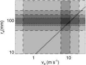
Parameter space defined by the corticocortical axonal range r _e and axonal velocity ν_e. Dashed lines indicate standard physiologic limits obtained from the literature, whereas dotted lines show model‐based constraints (see text for details). Dark shading indicates parameter zones that are consistent with multiple constraints.

The value of r _e in Figure 4 must lie below about one‐quarter of the circumference of the cortex, because this is an average range, and few if any fibers extend more than halfway around the cortex. Allowance for cortical folding relative to the skull circumference implies r _e ≲ 200 mm. Scaling of mouse data [Braitenberg and Schüz, 1998] to allow for the relative size of the human cortex gives 50 mm ≲ r _e ≲ 150 mm [Nunez, 1995], where we allow a significant uncertainty in Nunez's best estimate of 100 mm. In this and subsequent figures, the regions of parameter space that satisfy each of these constraints are shaded, with those that satisfy multiple constraints shaded darker.

Model‐based constraints are shown by dotted lines in Figure 4 and subsequent figures: consistency with the distance dependence of EEG coherence in human subjects yields r _e = 100 ± 20 mm [Robinson, 2003], whereas consistency with EEG spatial spectra implies r _e ≳ 70 mm [O'Connor et al., 2002]. The final constraint is of a different type: nonlinear least‐squares fits to EEG spectra of 100 normal adult subjects constrain the mean alert waking γ_e = v _e/r _e to the range 116 ± 4/s (mean ± standard error) [Rowe et al., 2003], which is indicated by the diagonal dotted lines in the figure.

Overall, it is seen that the model‐based constraints are consistent with those obtained by standard physiologic means, with the γ_e constraint complementing the other methods by cutting diagonally across the zone of parameter space that satisfies all the other constraints simultaneously. The zone that satisfies the entire set of constraints is a small trapezoidal strip with v _e = 9.8 ± 1.2 m/s, r _e = 89 ± 9 mm, and γ_e = 116 ± 4/s⁻¹.

Corticothalamic Loop Parameters

Figure 5a shows the space defined by the parameters R and V for an adult, the corticothalamic loop length and velocity, respectively. The velocity V is assumed to lie between the average unmyelinated and myelinated values, as for v _e. Steriade [1984] found values V = 4–11 m/s for thalamofugal fibers of various types, but we have not found values in the literature for corticothalamic fibers; Steriade's [1984] limits are indicated by dashed lines in Figure 5. Based on simple measurements of typical distances between cortical and thalamic sites in standard brain atlases, the typical loop length R must lie in the range 100–400 mm, as indicated in the figure. A further constraint to R > 150 mm is also shown, and discussed below. The time t ₀ = R/V required to make one circuit of the corticothalamic loop is bounded below by the one‐way travel times between cortex and thalamus, or vice versa, which are 2–20 ms in the cat (which scales to 5–60 ms for human brain dimensions) [Coenen, 1995; Koch, 1987; Steriade et al., 1997], yielding values of t ₀ twice as large. Estimates of t ₀ range from 5 ms to over 100 ms [Bal et al., 2000; Schmielau and Singer, 1977; Sillito et al., 1994]. Overall, we consolidate these estimates into bounds at 5 and 120 ms, shown by the diagonal dashed lines in Figure 5a.

Figure 5.

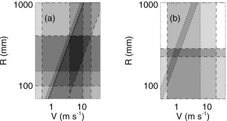
Parameter space defined by the corticothalamic loop length R and axonal velocity V. Dashed lines indicate standard physiologic limits obtained from the literature, whereas dotted lines show model‐based constraints (see text for details). Dark shading generally indicates parameter zones that are consistent with multiple constraints.

The model provides constraints on t ₀ = R/V. First, equation (22) implies t ₀ < T _α, which gives an upper bound of 111 msec, shown as a dotted diagonal line in Figure 5a, because the mean alpha frequency is over 9 Hz in adults [Nunez, 1995; Niedermeyer and Lopes da Silva, 1999]. Comparison with coherence data in children implies t ₀ < 90 ms [Robinson, 2003], giving another dotted diagonal bound, because t ₀ falls during development, in line with rising alpha frequency. Nonlinear least‐squares fitting to EEG spectra of 100 adult subjects (49 women, mean age 44 years, standard deviation 16 years; 51 men, mean age 45 years, standard deviation 15 years) implies a mean of t ₀ = 85 ± 1 ms, which yields two diagonal dotted lines in Figure 5a, which are almost indistinguishable on this scale [Rowe et al., 2003]. These model‐based constraints are consistent with those obtained by standard physiologic means, with the t ₀ constraint complementing the other methods and greatly restricting the allowable parameter combinations. The small trapezoidal zone that satisfies the entire set of constraints has V = 4.5 ± 0.5 m/s, R = 360 ± 40 mm, and t ₀ = 85 ± 1 ms.

A further constraint on R can be obtained by referring to Figure 5b, which is analogous to Figure 5a, but for newborn infants. In this case, the headsize, and hence R, is about 1.5 times smaller than for adults. The infant constraint t ₀ = 225 ± 50 ms imposed by the typical range of occipital α frequencies of 3.5–5 Hz [Lindsley, 1936, 1939; Smith, 1941] with α and β at adult values then selects a small zone at V ≃ 1.0 ± 0.5 m/s, consistent with low myelination in newborn infants. Scaling down the adult range of R by a factor of 1.5 implies R = 250 ± 30 mm, giving the further restriction to V ≃ 1.1 ± 0.4 m/s. The limit V < 6 m/s in newborns is also implied by the zone consistent with the adult constraints because myelination increases with age in children. Working in the reverse direction from the purely infant‐derived constraint R = 190 ± 90 mm immediately implies R ≥ 150 mm in Figure 5a, as shown previously with a dotted line.

Synaptodendritic Response Rates

Figure 6 shows the space defined by the combined synaptodendritic rate parameters α and β, i.e., the rates of decrease and increase of the resulting soma potential, respectively. In each frame we must have β > α by definition (otherwise the symbols are simply swapped to achieve this, without loss of generality). There is also an upper bound at α ≃ 500/s [Hestrin et al., 1990; Hestrin, 1993]. An upper bound is set at β = 2,500/s, again based on the results of Hestrin and coworkers [1990] for the shortest rise times seen at the soma. The rates corresponding to synaptic dynamics of AMPA, NMDA, GABA_A, and GABA_B receptors define the approximate locations of the corners of a quadrilateral, whose approximate location is shown in each frame [Bal et al., 1995; Dayan and Abbott, 2001; Destexhe and Mainen, 1994; Destexhe et al., 1996; Destexhe, 1998; Destexhe and Sejnowski, 2001; Dominguez‐Perrot et al., 1996; Lester and Jahr, 1992; Lumer et al., 1997] Given that neurotransmission in the brain is dominated by these four receptors, mean parameters should lie within this zone, or close to it. If dendritic cable properties lead to response rates at the soma that are smaller than those at the receptors, the location of the relevant corner of the quadrilateral is modified by replacing the receptor rate by the rate determined from the cable properties.

Figure 6.

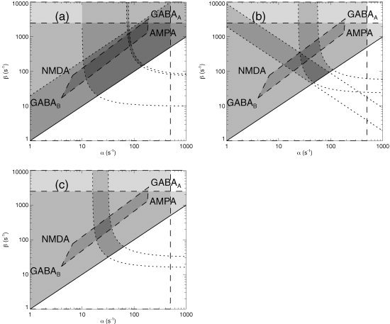
Parameter space defined by the rates β and α of soma potential rise and fall, respectively, allowing for combined synaptic and dendritic dynamics. Dashed lines indicate physiologic limits obtained from the literature, whereas dotted lines show model‐based constraints (see text for details), and the solid line bounds the unphysical region with β < α. Dark shading indicates parameter zones that are consistent with multiple constraints.

In Figure 6a, which corresponds to waking states, we show additional constraints that result from our model. The lowest curved dotted line is a lower bound on β imposed by equation (21) and the observation that the mean adult α period is approximately 100 ms. The pair of similar curves bound the range of possible combinations of α and β consistent with fits to observed alert, waking spectra, subject to holding T _α constant using equation (21) [Rowe et al., 2003]. Finally, an approximate upper bound β = 20α, obtained from fits, is shown as a dotted diagonal line [Rowe et al., 2003]. Rowe and associates [2003] found a wide scatter in estimates of this parameter, which had a mean of 8 and a median of 4. Only a small approximately rectangular zone satisfies all the constraints simultaneously. Overall, we conclude α = 80 ± 15/s and β = 800 ± 200/s for the eyes‐open state; corresponding values for the eyes‐closed, relaxed state are α = 65 ± 15/s and β = 550 ± 150/s.

Figure 6b corresponds to sleep stage 2, which is characterized by sleep‐spindle activity in the 7–15 Hz frequency range [Niedermeyer and Lopes da Silva, 1999]. In addition to the common constraints described above, Figure 6b shows a pair of parallel dotted lines, bounding the range of parameters consistent with spindle frequencies between 7 and 15 Hz, subject to equation (22). Simulations only reproduce observed sleep spectra [Robinson et al., 2002] if α is reduced to around 50/s for β = 4α; extrapolations to other values of β /α are shown by the two dotted curves, which bound the range that is semiquantitatively consistent with neurotransmitter data. Together, the constraints are only satisfied in a small triangle with α = 32 ± 8/s and β = 230 ± 70/s.

Figure 6c corresponds to slow‐wave sleep (stages 3 and 4), which is dominated by frequencies below about 2 Hz. It shows the model‐based constraints on α and β that result from requiring semiquantitative consistency with simulations and such sleep spectra, yielding α = 25 ± 8/s and β = 240 ± 150/s in this regime.

Overall, several points are notable from Figure 6. First, the model‐based constraints tend to complement the more traditional ones, cutting roughly perpendicular to them to define very small parameter zones of mutual consistency. In addition, the steady shift of the consistent zone toward lower left is consistent with the greater dominance of GABA_B receptor dynamics in sleep and the fall in response rates at low background firing rates [Destexhe and Sejnowski, 2001; Glenn and Steriade, 1982; Koch, 1999; Niedermeyer and Lopes da Silva, 1999; Steriade, 1984, 2000, 2001; Steriade et al., 1986, 1990a, b, 1997, 2001; Timofeev et al., 1996]. Recalling that α and β in our model are weighted averages over the corticothalamic system makes it plausible that this shift is more specifically due to GABA_B receptor dynamics in targets of reticular thalamic neurons [Destexhe and Sejnowski, 2001; Glenn and Steriade 1982; Niedermeyer and Lopes da Silva, 1999; Steriade, 1984, 2000, 2001; Steriade et al., 1986, 1990a, b, 1997, 2001; Timofeev et al., 1996], which is known to be more active in deep sleep than in waking, a point also consistent with our model's conclusions that the sign of feedback through the thalamus reverses in sleep [Robinson et al., 2001b, 2002, 2003a].

Firing Rates and Thresholds

Figure 7 shows the spaces defined by the maximum and mean firing rates of cortical, relay, and reticular neurons in the waking state. In each frame, there are bounds at Q _max = 100/s and 1,000/s, representing the physiologic range of maximal firing rates of individual neurons. There is also a bound at 500/s, in recognition of the fact that the firing rate averaged over subpopulations is unlikely to exceed this value if the maximum of any one subpopulation is less than 1,000/s, even leaving aside such effects as hypoxia if such high firing rates were sustained over whole populations. There are also diagonal lines at ϕ${}_{\mathit{\text{a}}}^{\text{(0)}}$ = Q _max because by definition, ϕ${}_{\mathit{\text{a}}}^{\text{(0)}}$ cannot exceed this bound. An upper bound at ϕ${}_{\mathit{\text{a}}}^{\text{(0)}}$ = 0.1Q _max is also indicated because the observation of increases of EEG signals by one to two orders of magnitude in seizures implies that the peak firing rate is at least one order of magnitude greater than the mean one. Further common bounds are seen at 7/s and 49/s, arising from equation (35) in conjunction with the observed firing rates. Finally, results from Figure 8 imply lower bounds at 0.009Q _max and 0.014Q _max, and upper bounds at 0.08Q _max and 0.27Q _max, as shown by dotted lines.

Figure 7.

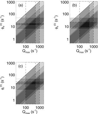
Parameter space defined by the maximum and steady‐state firing rates. Dashed lines indicate physiologic limits obtained from the literature, whereas dotted lines show model‐based constraints (see text for details), and the solid line bounds the unphysical region with Q _max < ϕ${}_{\mathit{\text{a}}}^{\text{(0)}}$. The uppermost diagonal bound is a superposition of both types of constraint. Dark shading indicates parameter zones that are consistent with multiple constraints. a: Cortex. b: Thalamic relay nuclei. c: Thalamic reticular nucleus.

Figure 8.

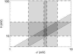
Parameter space defined by the spread in thresholds σ′ and the mean threshold relative to resting θ. Dashed lines indicate physiologic limits obtained from the literature, whereas dotted lines show model‐based constraints (see text for details). Dark shading indicates parameter zones that are consistent with multiple constraints.

Figure 7a shows additional bounds, obtained by Steriade et al. [2001] from intracellular recordings in cats (which should be similar to human values at the intracellular level), that restrict ϕ${}_{\mathit{\text{e}}}^{\text{(0)}}$ to the range 16 ± 2/s. In Figure 7b and c, limits ϕ${}_{\mathit{\text{s}}}^{\text{(0)}}$ = 16 ± 7 s⁻¹ and ϕ${}_{\mathit{\text{r}}}^{\text{(0)}}$ = 24 ± 5 s⁻¹ are shown, whereas values of the external stimuli lie in the range ϕ${}_{\mathit{\text{n}}}^{\text{(0)}}$ = 16 ± 4 s⁻¹ [Barrionuevo et al., 1981; Glenn and Steriade, 1982; Mukhametov et al., 1970; Steriade 1984, 2000, 2001; Steriade et al., 1986, 1990a, b, 1997; Timofeev et al., 1996]. Values as high as 36/s have been reported for ϕ${}_{\mathit{\text{r}}}^{\text{(0)}}$ [Mukhametov et al., 1970] but we use those from the analyses of Steriade and coworkers, which have the highest degree of methodologic consistency and compatibility across brain structures.

Because our model assumes a common value of Q _max, we find an overall mutually consistent range Q _max = 220–500/s from Figure 7a–c, with the above direct physiologic estimates of ϕ${}_{\mathit{\text{a}}}^{\text{(0)}}$ remaining unchanged.

Figure 8 shows the space defined by the variables σ′ and θ, with physiologic limits of 2–6 mV on σ′ and 10–25 mV on θ [Koch, 1999; Steriade et al., 2001], consistent with the fact that slow‐wave signals of around 20 mV peak‐to‐peak must be several times σ′ to suppress activity during the hyperpolarized phase of each cycle, as observed [Timofeev et al., 1996; Steriade et al., 2001], whereas the amplitudes of typical alpha waves (of a few mV) do not lead to strong nonlinear effects [Stam et al., 1999] (such effects are more common at larger amplitudes [Breakspear, 2002]). Exponential fits to the data in Figures 5 and 6 of Steriade and coworkers [2001] give σ′ = 3.8 ± 0.2 mV (mean ± standard error), as shown. This implies 2.5 < θ/σ′ < 6.2.

Steriade et al. [1997] have found slow‐wave sleep firing rates in thalamic relay nuclei to in the of order 4/s, which immediately implies ϕ₀ > 4/s, because these nuclei are believed to be inhibited in this state. Equations (35) and (36), together with the observed values of the ϕ${}_{\mathit{\text{a}}}^{\text{(0)}}$, imply 7/s < ϕ₀ < 18/s. Use of equations (35) and (36) then immediately implies 0.014ϕ${}_{\mathit{\text{a}}}^{\text{(0)}}$/Q _max < 0.27, as shown in Figure 7 by a pair of diagonal dotted lines. Hence, for Q _max in the above range, 0.014ϕ₀/Q _max < 0.08, and equation (34) and the result in the previous paragraph then combine to give θ/σ′ = 3.4 ± 0.9. This result and equation (35) then yield 0.009 < ϕ${}_{\mathit{\text{a}}}^{\text{(0)}}$/Q _max < 0.08, as shown by dotted lines in Figure 7.

Overall, from this section, we conclude σ′ = 3.8 ± 0.2 mV, θ = 10–17 mV, θ/σ′ = 3.4 ± 0.9, ϕ₀/Q _max = 0.014–0.1, and 0.014 < ϕ${}_{\mathit{\text{a}}}^{\text{(0)}}$/Q _max < 0.08.

Volume Conduction Versus Cortical Axonal Transmission

Two effects dominate lateral spreading of measured EEG signals: propagation across the cortex along long‐range fibers of characteristic length r _e, and volume conduction on scales ≲ 1/k ₀, where k ₀ is the corresponding low‐pass wavenumber. Figure 9 shows the space defined by k ₀ and r _e. Overall constraints on r _e from Figure 4 are shown as vertical lines, dotted because they rely on model‐based analyses. We are not aware of direct measurements of k ₀ in vivo, but modeling of volume conduction yields bounds k ₀ = 20–50/m [Nunez, 1981, 1995; Srinivasan et al., 1998]. Fits of our model to EEG coherence data imply k ₀ > 15/m [Robinson, 2003], fits to frequency spectra imply k ₀ r _e = 2–5 [Rowe et al., 2003], and fits to wavenumber spectra yield k ₀ r _e = 1–3. The latter two sets of bounds are shown as diagonal dotted lines in Figure 9. Overall, the constraints imply k ₀ = 29 ± 9/m and k ₀ r _e = 2.5 ± 0.5.

Figure 9.

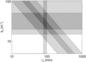
Parameter space defined by the mean corticocortical excitatory axonal range r _e and the volume conduction low‐pass wave number k ₀. Dotted lines show model‐based constraints (see text for details). Dark shading indicates parameter zones that are consistent with multiple constraints.

Synaptic Numbers, Strengths, Gains, and Related Quantities

Fits to 100 normal subjects yielded G _ee = 6.8 ± 0.2, G _ei = −8.1 ± 0.2, G _ese = 4.2 ± 0.2, G _esre = −3.1 ± 0.1, and G _srs = −0.37 ± 0.05 (mean ± standard error) [Rowe et al., 2003]. The discussion and references listed in connection with Figure 7 imply ϕ˜_e = ϕ${}_{\mathit{\text{e}}}^{\text{(0)}}$/ϕ₀ = 1 − 2.7, ϕ${}_{\mathit{\text{s}}}^{\text{(0)}}$/ϕ${}_{\mathit{\text{e}}}^{\text{(0)}}$ = 0.5 − 1.7, ϕ${}_{\mathit{\text{r}}}^{\text{(0)}}$/ϕ${}_{\mathit{\text{e}}}^{\text{(0)}}$ = 1.4 − 2.1, and ϕ${}_{\mathit{\text{n}}}^{\text{(0)}}$/ϕ${}_{\mathit{\text{e}}}^{\text{(0)}}$ = 0.7 − 1.3. By solving equations (41) to (46) for uniformly distributed random values in these ranges we obtain histograms of G _es, G _se, G _sr, G _sn, G _re, and G _rs, as seen in Figure 10. The half‐maximum points of these histograms depend only weakly on the endpoints of the ranges chosen, so we use them as the bounds on the ranges of the various G _ab, which are used in the analysis in Figure 11.

Figure 10.

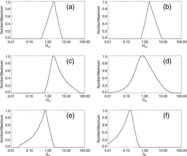
Histograms of gains obtained by Monte Carlo inversion of equations (41) to (46), using linear fit parameters from Rowe et al. [2003] and values of ϕ${}_{\mathit{\text{a}}}^{\text{(0)}}$ in physiologic ranges (see text). Each histogram is normalized by dividing by its maximum value. a: G _es. b: G _se. c: G _sr. d: G _sn. e: G _re. f: G _rs.

Figure 11.

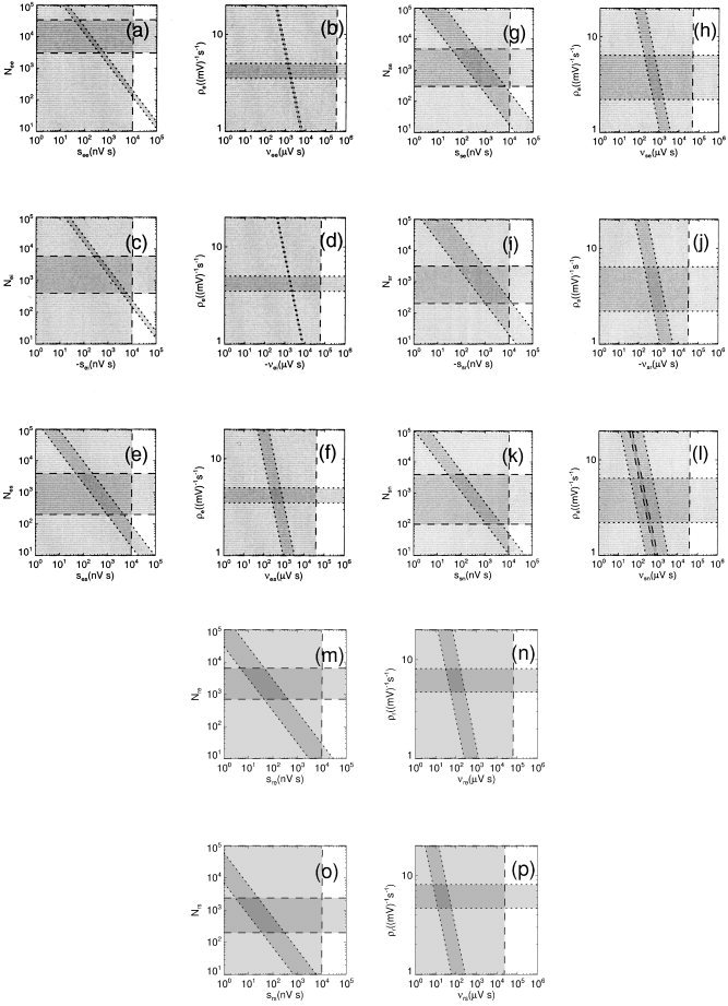
Parameter spaces defined by synaptic strengths s _ab and numbers of connections N _ab (left column) and by synaptic products v _ab and sigmoidal slopes ρ_a (right column). Dashed lines indicate standard physiologic limits obtained from the literature, whereas dotted lines show model‐based constraints (see text for details). Dark shading indicates parameter zones that are consistent with multiple constraints. a, b: ab = ee. c, d: ab = ei. e, f: ab = es. g, h: ab = se. i, j: ab = sr. k, l: ab = sn. m, n: ab = re. o, p: ab = rs.

Figure 11a shows the space defined by the mean number of excitatory‐to‐excitatory cortical synapses N _ee and their mean strength s _ee. A physiologic upper bound s _ee < 10 μV s is found from a weighted average of subclasses identified previously [Thomson et al., 1996; Thomson, 1997]. Complicating factors such as the effect of facilitation, experimental bias against detection of small postsynaptic potentials, reduced attenuation in vitro (normally arising in vivo from shorting of the dendritic membrane), variable channel‐opening probabilities, and temperature dependences of the dynamics make this only an approximation, and prevent the determination of a lower bound from these data. Bounds 3,000 < N _ee < 3.4 × 10⁴ are found from the fact that such synapses constitute 75–85% of the total of N _e = 4 × 10³ to 4 × 10⁴ synapses on cortical neurons [Braitenberg and Schüz, 1998; Douglas and Martin, 1998; Steriade et al., 1997]. The diagonal bounds, derived from Figure 11b and discussed below, represent constraints on the product ν_ab, which strongly restrict the allowable region to a narrow strip in parameter space.

Figure 11b shows the space defined by the product ν_ee = N _ee s _ee and the derivative ρ_e of the sigmoid, as defined by equation (8); for low firing rates, ρ_e ≈ ϕ${}_{\mathit{\text{a}}}^{\text{(0)}}$/σ′. Using the best estimates from Figures 7 and 8 implies ρ_e = 3.5–5.0/(mV s), which is broadly consistent with the estimate of 13.6/(mV s) in one instance by Koch [1999]. Bounds on ν_ee are found from the physiologically allowed rectangle in Figure 11a (i.e., ignoring the diagonal band there for now). The diagonal strip in Figure 11b is defined by the range of fitted values of G _ee = ρ_eν_ee. This strip immediately constrains ν_ee to a narrow range of values, which result in the diagonal bounds in Figure 11a. Overall, the constraints in Figure 11a and b imply N _ee = 3,000–3.4 × 10⁴, N _e = (4–40) × 10³, s _ee = 0.03–0.7 μV s, and ν_ee = 1.6 ± 0.4 mV s. This implies that the values obtained previously for s _ee in vitro [Thomson et al., 1996; Thomson, 1997] are indeed overestimates, probably for the reasons mentioned above.

Figures 11c and d are analogous to 11a and b, but for inhibitory‐to‐excitatory cortical synapses. The number N _ei is 10–15% of N _e, whereas measurements imply −s _ei < 10 μV s. The same reasoning as before then yields N _ei = 400–6,000, s _ee = −(0.3–6) μV s, and ν_ei = −(2.0 ± 0.5) mV s.

Figures 11e and f are for thalamocortical relay‐to‐excitatory synapses. The number N _es is 5–10% of N _e [Sherman and Koch, 1988], whereas we assume the same bounds on s _es as on the other synaptic strengths. The above reasoning then yields N _es = 200–4,000, s _es = 0.05–5 μV s, and ν_es = 0.3–1.4 mV s.

Figure 11g–p follow the same line of reasoning as for synapses afferent on cortical excitatory neurons, using constraints from the third column of Table I and yielding those in the fourth column. In each case, initial physiologic upper bounds on the |s _ab| have been set to 10 μV s. The numbers of synaptic connections have been estimated from mean total synaptic numbers N _s and N _r and mean fractions of each type, as summarized in the third column of Table I [Jones, 1985; Sherman and Koch, 1988; Liu et al., 1995a, b; Erişir et al., 1997; Steriade et al., 1997; Kim and McCormick, 1998; Braitenberg and Schüz, 1998; Liu and Jones, 1999; Steriade, 2001; Sherman and Guillery, 2001], whereas bounds on ρ_a are drawn from the results in Figures 7 and 8. In addition, Coenen [1995] estimated G _sn = 0.7–1.0, which is shown in Figure 11(l) as a pair of diagonal dashed lines.

The constraints implied by equations (30) to (32) are obeyed by the values obtained from Figure 11, with the |ν_ab| all less than a few mV s. Significantly, the final values of the ν_ab are much better constrained than are those of the N _ab or s _ab separately. Only the ν_ab affect the dynamics.

In some cases, ratios of quantities such as the s _ab can be better constrained than individual values. For example, by writing |s _ei|/s _ee = (|ν_ei|/ν_ee)(N _ee/N _ei), one finds an estimate of 8 for this ratio (range, 4–18) from the constraints on the quantities on the right of this equation. In contrast, the upper bounds on s _ee and |s _ei| do not constrain their ratio.

The same arguments as in the previous paragraph can be used to constrain the ratio s _es/s _ee, giving a best estimate of around 2.6, with a range of 0.75–14. This is in good agreement with results quoted by Zador [1999], who noted that thalamocortical excitatory synapses are “more than twice as strong“ as intracortical ones on average.

Self‐Consistent Nominal Case

For many purposes, it is useful to have a specific set of nominal parameters that sit near the center of the zone that satisfies all the constraints simultaneously, and that are mutually self‐consistent. One such set of parameters is given in the fifth column of the Table I. It must be stressed that these parameters are only representative of the allowed ranges and the actual values are likely to differ somewhat.

DISCUSSION

We have used a model‐based analysis of EEG‐related data, in tandem with standard physiologic and anatomic measures, to constrain a large number of average parameters, primarily of the normal adult brain in an alert, eyes‐open state. Results obtained from our physiologically based model are both consistent with and complementary to independent measures. In many cases, the importance and utility of particular parameters is only apparent within the framework provided by the model.

Use of multiple constraints in tandem, while requiring mutual consistency, has proved to be a powerful approach, which yields far tighter overall constraints than can be obtained by standard means, with our final parameter estimates summarized in Table I. Significantly, mutual consistency across multiple different parameters can only be imposed within the framework of a model that interrelates them. Moreover, when combinations of parameters (e.g., products or quotients) are constrained, the allowable parameter space is often reduced greatly, even though allowable ranges of the individual parameters may not be. Ultimately, the boundaries obtained should be viewed as approximate, because they apply to group averages and also involve inferences from multiple data sources, not all human; parameters of individuals, and possibly even group averages, may well lie slightly outside these limits.

Although we deal here only with average values of a relatively small number of parameters, many of these can be constrained via fits to data from individual subjects. Moreover, trends in the averaged parameters may yield clues as to underlying mechanisms, or may indicate directions in which more detailed parametrizations might be pursued usefully. So far, we have trodden a middle road between having a model that is too simple to be realistic on one hand, and parametrizing every conceivable piece of relevant anatomy and physiology at the expense of having many undetermined parameter values on the other. The excellent agreement in previous studies with data from a variety of experiments and with independent physiologic estimates discussed here indicates that the version of the model used provides a good approximation to the most relevant features of physiology and anatomy. It is not intended to be exhaustive, and the parameters it yields are implicitly effective values that average over subcases that the model does not distinguish.

It might be asked why the methods used here are generally more effective at obtaining averaged quantities than direct physiologic approaches. The reason is that in EEG phenomena, nature does the averaging, because EEG signals are intrinsically the product of many neuronal signals. An effective model can exploit this self‐averaging to effectively sample far larger populations than is practical during direct in vivo or in vitro studies, but this does not dispense with the need for independent verification via such measurements, at least for now. The large populations of subjects used in some of the statistical studies (e.g., the linear fits to normal adult EEG spectra) also assist in reducing statistical fluctuations by more conventional means.

The results here probe spatial scales ranging from the synaptic level to the whole brain, and temporal scales from milliseconds to seconds or more. As mentioned above, we have concentrated on average values to provide an initial demonstration of the power and utility of our approach. However, there are many directions in which this analysis could be generalized. For example, changes in parameters with arousal, development, disorder, cognition, and drug administration could be explored, as could the effects of seizure, hypoxia, and other regimes. Studies of temporal dynamics of the parameters are also feasible, and we have produced recently the first topographic maps of the linear EEG fit parameters [Robinson et al., 2003b]. Prediction of additional phenomena from the model, such as seizure dynamics, nonlinear correlations, and the BOLD response, should also lead to further constraints.

New quantitative physiologic and anatomic studies (or reanalysis of existing ones, including ones overlooked by us in our searches of the vast literature on these topics) would be particularly valuable to test the model in more detail, and we hope that the present analysis will stimulate further work along these lines. For example, constraints on the gains G _ab can be obtained by measuring average transfer ratios (pulses out per pulse in) for various neural populations [Coenen, 1995], whereas many of the parameters in Table I are directly measurable but need to be averaged over large populations in vivo. Improved estimates of the steady‐state firing rates as functions of arousal and disorder would be particularly valuable. Less conventionally, our use of mutual consistency permits some quite nonstandard approaches to constraining parameters to be used. For example, better measures of the synaptic numbers N _ab or gains G _ab may provide the best way to constrain the synaptic strengths s _ab, which are extremely hard to measure in vivo.

The relatively large‐scale brain activity, whose parameters are discussed here, is both the overall manifestation of and the potentiating background to the fine‐scale information processing of the brain. Understanding its features is essential to understanding the finer‐scale phenomena. An analogy from physics is the behavior of the large‐scale magnetic field of a magnetic material: this field results from the alignment of microscopic nuclear magnets, but also self‐consistently determines this very degree of alignment itself.

REFERENCES

- Bal T, Debay D, Destexhe A (2000): Cortical feedback controls the frequency and synchrony of oscillations in the visual thalamus. J Neurosci 20: 7478–7488. [DOI] [PMC free article] [PubMed] [Google Scholar]
- Bal T, von Krosigk M, McCormick DA (1995): Synaptic and membrane mechanisms underlying synchronized oscillations in the ferret lateral geniculate nucleus in vitro. J Physiol 483.3: 641–663. [DOI] [PMC free article] [PubMed] [Google Scholar]
- Barrionuevo G, Benoit O, Tempier P (1981): Evidence for two types of firing pattern during the sleep‐waking cycle in the reticular thalamic nucleus of the cat. Exp Neurol 72: 486–501. [DOI] [PubMed] [Google Scholar]
- Braitenberg V, Schüz A (1998): Cortex: statistics and geometry of neuronal connectivity (2nd ed). Berlin: Springer. [Google Scholar]
- Breakspear M (2002): Nonlinear phase desynchronization in human electroencephalographic data. Hum Brain Mapp 15: 175–198. [DOI] [PMC free article] [PubMed] [Google Scholar]
- Coenen AML (1995): Neuronal activities underlying the electroencephalogram and evoked potentials of sleeping and waking: implications for information processing. Neurosci Biobehav Rev 19: 447–463. [DOI] [PubMed] [Google Scholar]
- Dayan P, Abbott LF (2001): Theoretical neuroscience: computational and mathematical modeling of neural systems. Cambridge: MIT. [Google Scholar]
- Destexhe A (1998): Spike‐and‐wave oscillations based on the properties of GABAB receptors. J Neurosci 18: 9099–9111. [DOI] [PMC free article] [PubMed] [Google Scholar]
- Destexhe A, Bal T, McCormick DA, Sejnowski TJ (1996): Ionic mechanisms underlying synchronized oscillations and propagating waves in a model of ferret thalamic slices. J Neurophysiol 76: 2049–2070. [DOI] [PubMed] [Google Scholar]
- Destexhe A, Mainen ZF (1994): Synthesis of models for excitable membranes, synaptic transmission and neuromodulations using a common kinetic formalism. J Comp Neurosci 1: 195–230. [DOI] [PubMed] [Google Scholar]
- Destexhe A, Sejnowski TJ (2001): Thalamocortical assemblies: how ion channels, single neurons, and large‐scale networks organize sleep oscillations. Oxford: Oxford. [Google Scholar]
- Dominguez‐Perrot C, Feltz P, Poulter MO (1996): Recombinant GABAA receptor desensitization: the role of the γ2 subunit and its physiological significance. J Physiol 497: 145–159. [DOI] [PMC free article] [PubMed] [Google Scholar]
- Douglas R, Martin K (1998): Neocortex In: Shepherd GM, editor. The synaptic organization of the brain (4th ed). Oxford: Oxford University Press. [Google Scholar]
- Erişir A, Van Horn S, Sherman, SM (1997): Relative numbers of cortical and brainstem inputs to the lateral geniculate nucleus. Proc Nat Acad Sci USA 94: 1517–1520. [DOI] [PMC free article] [PubMed] [Google Scholar]
- Freeman WJ (1975): Mass action in the nervous system. New York: Academic. [Google Scholar]
- Freeman WJ (1992): Tutorial on neurobiology: from single neurons to brain chaos. Int J Bifurcation Chaos 2: 451–482. [Google Scholar]
- Glenn LL, Steriade M (1982): Discharge rate and excitability of cortically projecting intralaminar thalamic neurons during waking and sleep states. J Neurosci 10: 1387–1404. [DOI] [PMC free article] [PubMed] [Google Scholar]
- Hestrin S (1993): Different glutamate receptor channels mediate fast excitatory synaptic currents in inhibitory and excitatory cortical neurons. Neuron 11: 1083–1091. [DOI] [PubMed] [Google Scholar]
- Hestrin S, Sah P, Nicoll RA (1990): Mechanisms generating the time course of dual component excitatory synaptic currents recorded in hippocampal slices. Neuron 5: 247–253. [DOI] [PubMed] [Google Scholar]
- Jirsa VK, Haken H (1996): Field theory of electromagnetic brain activity. Phys Rev Lett 77: 960–963. [DOI] [PubMed] [Google Scholar]
- Jones EG (1985): The thalamus. New York: Plenum Press. [Google Scholar]
- Kandel ER, Schwartz JH, Jessell TM (1991): Principles of neural science (3rd Ed). Norwalk: Appleton and Lange. [Google Scholar]
- Kim U, McCormick DA (1998): The functional influence of burst and tonic firing mode on synaptic interactions in the thalamus. J Neurosci 18: 9500–9516. [DOI] [PMC free article] [PubMed] [Google Scholar]
- Koch C (1987): The action of the corticofugal pathway on sensory thalamic nuclei: a hypothesis. Neuroscience 23: 399–406. [DOI] [PubMed] [Google Scholar]
- Koch C (1999): Biophysics of computation. New York: Oxford University Press. [Google Scholar]
- Lester RAJ, Jahr CE (1992): NMDA channel behavior depends on agonist affinity. J Neurosci 12: 635–643. [DOI] [PMC free article] [PubMed] [Google Scholar]
- Lindsley DB (1936): Brain potentials in children and adults. Science 84: 354. [DOI] [PubMed] [Google Scholar]
- Lindsley DB (1939): A longitudinal study of the occipital alpha rhythms in normal children: Frequency and amplitude standards. J Genet Psychol 55: 197–215. [Google Scholar]
- Liu XB, Honda CN, Jones EG (1995a): Distribution of four types of synapse on physiologically identified relay neurons in the ventral posterior thalamic nucleus of the cat. J Comp Neurol 352: 69–91. [DOI] [PubMed] [Google Scholar]
- Liu XB, Jones EG (1999): Predominance of corticothalamic synaptic inputs to thalamic reticular nucleus neurons in the rat. J Comp Neurol 414: 67–79. [PubMed] [Google Scholar]
- Liu XB, Warren RA, Jones EG (1995b): Synaptic distribution of afferents from reticular nucleus in ventroposterior nucleus of cat thalamus. J Comp Neurol 352: 187–202. [DOI] [PubMed] [Google Scholar]
- Lopes da Silva FH, Hoeks A, Smits H, Zetterberg LH (1974): Model of brain rhythmic activity. The alpha rhythm of the thalamus. Kybernetik 15: 27–37. [DOI] [PubMed] [Google Scholar]
- Lopes da Silva FH, van Rotterdam A, Barts P, van Heusden E, Burr W (1976): Models of neuronal populations: the basic mechanisms of rhythmicity. Prog Brain Res 45: 281–308. [DOI] [PubMed] [Google Scholar]
- Lopes da Silva FH, Vos JE, Mooibroek J, van Rotterdam A (1980): Relative contributions of intracortical and thalamocortical processes in the generation of alpha rhythms, revealed by partial coherence analysis. Electroencephalogr Clin Neurophysiol 50: 449–456. [DOI] [PubMed] [Google Scholar]
- Lumer ED, Edelman GM, Tononi G (1997): Neural dynamics in a model of the thalamocortical system: I. Layers, loops and the emergence of fast synchronous rhythms. Cereb Cortex 7: 207–227. [DOI] [PubMed] [Google Scholar]
- Mukhametov LM, Rizzolatti G, Tradardi V (1970): Spontaneous activity of neurones of nucleus reticularis thalami in freely moving cats. J Physiol 210: 651–667. [DOI] [PMC free article] [PubMed] [Google Scholar]
- Niedermeyer E, Lopes da Silva FH (1999): Electroencephalography: basic principles, clinical applications, and related fields (4th ed). Baltimore: Williams and Wilkins. [Google Scholar]
- Nunez PL (1974): Wavelike properties of the alpha rhythm. IEEE Trans Biomed Eng 21: 473–482. [Google Scholar]
- Nunez PL (1981): Electric fields of the brain. Oxford: Oxford University Press. [Google Scholar]
- Nunez PL (1995): Neocortical dynamics and human EEG rhythms. Oxford: Oxford University Press. [Google Scholar]
- Nunez PL (2000): Toward a quantitative description of large‐scale neocortical dynamic function and EEG. Behav Brain Sci 23: 371–437. [DOI] [PubMed] [Google Scholar]
- O'Connor SC, Robinson PA (2003a): Wave‐number spectrum of electrocorticographic signals. Phys Rev E Phys 67: 051912; 1–12. [DOI] [PubMed] [Google Scholar]
- O'Connor SC, Robinson PA (2003b): Unifying and interpreting the spectral wavenumber content of EEGs, ECoGs, and ERPs. J Theor Biol (submitted). [DOI] [PubMed]
- O'Connor SC, Robinson PA, Chiang AK (2002): Wave‐number spectrum of electroencephalographic signals. Phys Rev E Phys 66: 061905; 1–12. [DOI] [PubMed] [Google Scholar]
- Rennie CJ, Robinson PA, Wright JJ (1999): Effects of local feedback on dispersion of electrical waves in the cerebral cortex. Phys Rev E Stat Nonlin Soft Matter Phys 59: 3320–3329. [Google Scholar]
- Rennie CJ, Robinson PA, Wright JJ (2002): Unified neurophysical model of EEG spectra and evoked potentials. Biol Cybern 86: 457–471. [DOI] [PubMed] [Google Scholar]
- Rennie CJ, Wright JJ, Robinson PA (2000): Mechanisms of cortical electrical activity and emergence of gamma activity. J Theor Biol 205: 17–35. [DOI] [PubMed] [Google Scholar]
- Robinson PA (2003): Neurophysical theory of coherence and correlations of electroencephalographic and electrocorticographic signals. J Theor Biol 222: 163–175. [DOI] [PubMed] [Google Scholar]
- Robinson PA, Loxley PN, O'Connor SC, Rennie CJ (2001a): Modal analysis of corticothalamic dynamics, electroencephalographic spectra, and evoked potentials. Phys Rev E Phys 63: 041909; 1–13. [DOI] [PubMed] [Google Scholar]
- Robinson PA, Rennie CJ, Rowe DL (2002): Dynamics of large‐scale brain activity in normal arousal states and epileptic seizures. Phys Rev E Phys 65: 041924; 1–9. [DOI] [PubMed] [Google Scholar]
- Robinson PA, Rennie CJ, Rowe DL, O'Connor SC, Wright JJ, Gordon E, Whitehouse RW (2003a): Neurophysical modeling of brain dynamics. Neuropsychopharmacology 28(Suppl): 74–79. [DOI] [PubMed] [Google Scholar]
- Robinson PA, Rennie CJ, Wright JJ (1997): Propagation and stability of waves of electrical activity in the cerebral cortex. Phys Rev E Phys 56: 826–840. [Google Scholar]
- Robinson PA, Rennie CJ, Wright JJ, Bahramali H, Gordon E, Rowe DL (2001b): Prediction of electroencephalographic spectra from neurophysiology. Phys Rev E Phys 63: 021903; 1–18. [DOI] [PubMed] [Google Scholar]
- Robinson PA, Rennie CJ, Wright JJ, Bourke PD (1998): Steady states and global dynamics of electrical activity in the cerebral cortex. Phys Rev E Phys 58: 3557–3571. [Google Scholar]
- Robinson PA, Rowe DL, Rennie CJ, O'Connor SC, Breakspear M, Gordon E (2003b): Multiscale brain modeling. Oral presentation and Poster 935, Human Brain Mapping Conference, New York. Neuroimage 19(Suppl): 46. [Google Scholar]
- Robinson PA, Whitehouse RW, Rennie CJ (2003c): Nonuniform corticothalamic continuum model of electroencephalographic spectra with application to split alpha peaks. Phys Rev E Phys 68: 021922; 1–10. [DOI] [PubMed] [Google Scholar]
- Rowe DL, Robinson PA, Rennie CJ, Powles RC (2003): Estimation of neurophysiological parameters from the waking EEG using a biophysical model of brain dynamics. J Theor Biol (submitted). [DOI] [PubMed]
- Schmielau F, Singer W (1977): The role of visual cortex for binocular interactions in the cat lateral geniculate nucleus. Brain Res 120: 354–361. [DOI] [PubMed] [Google Scholar]
- Sherman SM, Guillery RW (2001): Exploring the thalamus. San Diego: Academic Press. [Google Scholar]
- Sherman SM, Koch C (1988): Thalamus In: Shepherd GM, editor. The synaptic organization of the brain. Oxford: Oxford University Press. [Google Scholar]
- Sillito AM, Jones HE, Gerstein GL, West DC (1994): Feature‐linked synchronization of thalamic relay cell firing induced by feedback from the cortex. Nature 369: 479–482. [DOI] [PubMed] [Google Scholar]
- Smith JR (1941): The frequency growth of the human alpha rhythms during normal infancy and childhood. J Psych 11: 177–198. [Google Scholar]
- Srinivasan R, Nunez PL, Silberstein RB (1998): Spatial filtering and neocortical dynamics: estimates of EEG coherence. IEEE Trans Biomed Eng 45: 814–826. [DOI] [PubMed] [Google Scholar]
- Stam CJ, Pijn JPM, Suffczynski P, Lopes da Silva FH (1999): Dynamics of the human alpha rhythm: evidence for nonlinearity? Clin Neurophysiol 110: 1801–1813. [DOI] [PubMed] [Google Scholar]
- Steriade M (1984): The excitatory‐inhibitory response sequence in thalamic and neocortical cells: state‐related changes and regulatory systems In: Edelman GM, Gall WE, Cowan WM. Dynamical aspects of neocortical function. New York: Wiley; p 107–157. [Google Scholar]
- Steriade M (2000): Corticothalamic resonance, states of vigilance and mentation. Neuroscience 101: 243–276. [DOI] [PubMed] [Google Scholar]
- Steriade M (2001): The intact and sliced brain. Cambridge: MIT Press. [Google Scholar]
- Steriade M, Datta S, Oakson G, Curró Dossi R (1990a): Neuronal activities in brainstem cholinergic nuclei related to tonic activation processes in thalamocortical systems. J Neurosci 10: 2541–2559. [DOI] [PMC free article] [PubMed] [Google Scholar]
- Steriade M, Domich L, Oakson G (1986): Reticularis thalami neurons revisited: activity changes during shifts in states of vigilance. J Neurosci 6: 68–81. [DOI] [PMC free article] [PubMed] [Google Scholar]
- Steriade M, Gloor P, Llinás RR, Lopes da Silva FH, Mesulam M‐M (1990b): Basic mechanisms of cerebral rhythmic activities. Electroencephalogr Clin Neurophysiol 76: 481–508. [DOI] [PubMed] [Google Scholar]
- Steriade M, Jones EG, McCormick DA (1997): Thalamus (2 volumes). Oxford: Elsevier. [Google Scholar]
- Steriade M, Timofeev I, Grenier F (2001): Natural waking and sleep states: a view from inside neocortical neurons. J Neurophysiol 85: 1969–1985. [DOI] [PubMed] [Google Scholar]
- Thomson AM (1997): Activity‐dependent properties of synaptic transmission at two classes of connections made by rat neocortical pyramidal axons in vitro. J Physiol (Lond) 502.1: 131–147. [DOI] [PMC free article] [PubMed] [Google Scholar]
- Thomson AM, West DC, Hahn J, Deuchars J (1996): Single axon IPSPs elicited in pyramidal cells by three classes of interneurons in slices of rat cortex. J Physiol (Lond) 496.1: 81–102. [DOI] [PMC free article] [PubMed] [Google Scholar]
- Timofeev I, Contreras D, Steriade M (1996): Synaptic responsiveness of cortical and thalamic neurones during various phases of slow sleep oscillation in cat. J Physiol 494.1: 265–278. [DOI] [PMC free article] [PubMed] [Google Scholar]
- Valdes PA, Jimenez JC, Riera J, Biscay R, Ozaki T (1999): Nonlinear EEG analysis based on a neural mass model. Biol Cybern 81: 415–424. [DOI] [PubMed] [Google Scholar]
- Wendling F, Bartolomei F, Bellanger JJ, Chauvel P (2001): Interpretation of interdependencies in epileptic signals using a macroscopic physiological model of the EEG. Clin Neurophysiol 112: 1201–1218. [DOI] [PubMed] [Google Scholar]
- Wendling F, Bartolomei F, Bellanger JJ Chauvel P (2002): Epileptic fast activity can be explained by a model of impaired GABAergic inhibition. Eur J Neurosci 15: 1499–1508. [DOI] [PubMed] [Google Scholar]
- Wendling F, Bellanger JJ, Bartolomei F, Chauvel P (2000). Relevance of nonlinear lumped‐parameter models in the analysis of depth‐EEG epileptic signals. Biol Cybern 83: 367–378. [DOI] [PubMed] [Google Scholar]
- Wilson HR, Cowan JD (1973): A mathematical theory of the functional dynamics of cortical and thalamic nervous tissue. Kybernetik 13: 55–80. [DOI] [PubMed] [Google Scholar]
- Wright JJ (1999): Simulation of the EEG: dynamic changes in synaptic efficacy, cerebral rhythms, and dissipative and generative activity in cortex. Biol Cybern 81: 131–147. [DOI] [PubMed] [Google Scholar]
- Wright JJ, Liley DTJ (1996): Dynamics of the brain at global and microscopic scales: neural networks and the EEG. Behav Brain Sci 19: 285–320. [Google Scholar]
- Zador A (1999): Thalamocortical synapses: sparse but stentorian. Neuron 23: 198–200. [DOI] [PubMed] [Google Scholar]
- Zetterberg LH, Kristiansson L, Mossberg K (1978): Performance of a model for a local neuron population. Biol Cybern 31: 15–26. [DOI] [PubMed] [Google Scholar]