

Abstract
We evaluated the rapid changes in regional scalp EEG synchronization in normal subjects with spatial and temporal resolution exceeding prior art 10‐fold with a high spatial density array and the Hilbert transform. A curvilinear array of 64 electrodes 3 mm apart extending 18.9 cm across the scalp was used to record EEG at 200/sec. Analytic amplitude (AA) and phase (AP) were calculated at each time step for the 64 traces in the analog pass band of 0.5–120 Hz. AP differences approximated the AP derivative (instantaneous frequency). The AP from unfiltered EEG revealed no reproducible patterns. Filtering was necessary in the β and gamma ranges according to a technique that optimized the correlation of the AP differences with the activity band pass filtered in the alpha range. The sizes of temporal AP differences were usually within ±0.5 radian from the average step corresponding to the center frequency of the pass band. Large AP differences were often synchronized over distances of 6 to 19 cm. An optimal pass band to detect and measure these recurring jumps in AP in the β and γ ranges was found by maximizing the α peak in the cospectrum of the correlation between unfiltered EEG and the band pass AP differences. Synchronized AP jumps recurred in clusters (CAP) at α and theta rates in resting subjects and with EMG. Cortex functions by serial changes in state. The Hilbert transform of EEG from high‐density arrays can visualize these state transitions with high temporal and spatial resolution and should be useful in relating EEG to cognition. Hum. Brain Mapping 19:248–272, 2003. © 2003 Wiley‐Liss, Inc.
Keywords: Hilbert transform, neurodynamics, phase re‐setting, state transition, scalp EEG, scalp EMG, synchronization of beta‐gamma
INTRODUCTION
The genesis and control of behavior requires the coordination of diverse areas of cerebral cortex interacting with the subcortical structures. Well‐defined behavioral states require sequential epochs of cortical activity, in which the neural activity in multiple cortical areas is formed by cooperation and expressed in spatial patterns. Studies of intracranial EEG from high‐density electrode arrays implanted in animals on sensory cortices revealed episodic spatial patterns of amplitude and phase modulation (AM and PM) of carrier waves in the γ range [Freeman, 2000a] from primary sensory areas: olfactory [Freeman and Viana Di Prisco, 1986; Freeman and Grajski, 1987], visual [Freeman and van Dijk, 1987], auditory [Ohl et al., 2001], and somatomotor [Barrie et al., 1996]. These epochs were denoted “wave packets” [Freeman, 1975]. The AM patterns were related to conditioned stimuli (CS) that the animals had been trained to discriminate. The PM had the stereotypic form of a radially symmetric phase gradient. The isophase contours indicated the form of a cone, when phase values were plotted in the two surface dimensions of the cortex. This pattern resembled the spreading wave from a pebble dropped in water. It indicated that the cortical states expressed in AM patterns formed abruptly and replaced prior patterns in rapid succession at rates in the θ and δ ranges [Freeman and Baird, 1987; Freeman and Barrie, 2000, Freeman, 2003b]. The statistical relation of the patterns to conditioned stimuli indicated that the neural activity manifesting AM patterns was involved in the genesis and control of discriminative behavior.
These results were based on the Fourier transform. The temporal resolution for investigating the manner of pattern change was limited by the necessity for defining the frequency over a time interval long enough to include at least one cycle of each frequency [Freeman, 2003b]. This limitation prevented examining rapid changes in phase patterns. The limitation was overcome by using the Hilbert transform [Barlow, 1993; Pikovsky et al., 2001; Tass et al., 1999], which transformed time series data into a vector by decomposing it into two independent time series, one for the analytic amplitude (AA) and the other for the instantaneous analytic phase (AP). The calculation of phase was modulo π or 2π, so the phase has the appearance of a sawtooth function. For segments of arbitrary duration, the phase was unwrapped to display it as continuously varying with time. The frequency is given by the slope of the function, either in the local vicinity of each digitized value or averaged over any convenient time window. Thus, phase was derived before frequency from EEG with high temporal resolution, limited only by the digitizing rate, in contrast to the Fourier method, in which phase followed frequency decomposition with high frequency resolution but poor temporal resolution [Le Van Quyen et al., 2001; Quiroga et al., 2002].
The results from applying the Hilbert method to the animal data [Freeman and Rogers, 2002] confirmed the prediction of finding local epochs of stable phase patterns that were punctuated by abrupt changes in AA and AP in the multiple traces. These abrupt changes together revealed a transition from one state to another state of the cortical dynamics. The sequential AP jumps were approximately synchronized over the recording areas, with directions of change in analytic phase (− or +, lead or lag) that varied randomly with time and location. This variation was in accord with the formation at each cortical state change of a new phase cone with its apex having a new sign and location. The Hilbert transform made it possible to evaluate the degree of synchrony within an area of cortex, which was based in the stabilization of a non‐zero distribution of AP values in a conic pattern. This was done by using an index of pairwise synchrony derived by Tass et al. [ 1998] from Shannon entropy that was applied to the phase distributions. That index was generalized to multiple traces within each cortical area [Freeman and Rogers, 2002] and then extended to an evaluation of synchrony over traces from multiple cortical areas [Freeman and Rogers, 2003].
The clean separation of the AP and AA by the Hilbert transform appeared suitable for application to human scalp EEG for improved temporal resolution in search of evidence for episodic changes in cortical states that resembled wave packets. However, the AP and AA were not interpretable when the Hilbert transform was applied to noisy, broad band signals from multiple recording sites. A salient aim of the present study was improve on methods for applying the Hilbert transform to human scalp EEG in order to measure and interpret the rapid changes in synchrony between multiple areas of the brain that are thought to occur during cognitive behavior [Bressler, 1995; Haig et al., 2000; Lachaux et al., 1999; Miltner et al., 1999; Müller et al., 1996; Müller, 2000; Rodriguez et al., 1999; Tallon‐Baudry et al., 1996, 1998; Varela et al., 2001].
METHODS AND THEIR RATIONALES
Subjects were five male and four female adult volunteers, who were asked to sit quietly and relax their muscles, first with eyes closed and then with eyes open. Records free of movement artifacts were selected by off‐line editing. For comparison, records were also selected in periods of EMG activity deliberately induced by tensing the scalp. The data were collected in the EEG Clinic of Harborview Hospital, University of Washington, Seattle, and were sent by ftp without identifying markers of personal information to the University of California at Berkeley for analysis. The data collection and management were governed by protocols approved by the Helsinki Declaration and the Institutional Review Boards in both institutions.
A curvilinear electrode array was made with 64 gold‐plated needles threaded into a band of embroidery fabric with interstices at 3‐mm intervals for a length of 18.9 cm. The scalp was cleaned and dried, and the array was bound firmly onto the forehead across the midline just below the frontal hairline, paracentrally along the part line, or across the occiput. Recordings were referential all with respect to the same reference electrode either on the vertex for frontal and occipital recording or on the contralateral mastoid for paracentral recording. The ground was located on the contralateral mastoid for frontal and paracentral recording, and on the frontal midline (AFz) for occipital recording. The EEG were amplified with a Nicolet (BMSI 5000) system having a fixed gain of 1,628 and analog filters set at 0.5 Hz high pass and 120 Hz low pass. The ADC gave 12 bits with the least significant bit of 0.9 μV and a maximal range 4,096 bits. Possible DC amplifier offsets were removed off‐line by subtracting the channel means of each entire recording. The digitizing rate was 200 samples/sec (5‐msec interval), while the analog filter was set at 120 Hz. Due to the possibility of aliasing between 80–100 Hz, that part of the temporal spectrum was ignored. The data for each subject and condition were blocked into matrices of 5,000 data points. Temporal power spectral densities (PSDt) were calculated with the 1‐D FFT for every channel after applying a Hanning window to epochs usually of 1 sec, nonoverlapping, and ranging from 0.1 sec to the full duration of each block for each of the 64 EEG. The 64 PSDt were averaged and transformed for display in log‐log coordinates [Freeman et al., 2003].
Most of the data processing was done with MATLAB software, including convolution in the time domain for temporal filtering with finite impulse response (FIR) filters estimated using Parks‐McClellan algorithm of order 200. The transition band width was 4 Hz, except in the cases of narrow adjacent temporal filters, where the transition band width was 1 Hz. Special purpose software was developed for spatial filtering [Freeman and Baird, 1987] of the EEG in the spatial frequency domain. The 1‐D FFT was applied to the 64 digitized EEG amplitudes at each time point to get the spatial power spectral density (PSDX). The spectrum was multiplied by an exponential filter, and the inverse FFT was taken of the real and imaginary parts of the spectrum to get the filtered spatial patterns. An exponential low‐pass filter was used [Gonzalez and Wintz, 1977] with the factor for attenuation, A(fx), ranging from 1 and 0 with increasing spatial frequency, fx, by
| (1) |
where fo was the cut‐off frequency, n = 2. The same equation held for a high pass filter with n = −6 with A(fx) ranging from 0 to 1 with increasing frequency. The effect on the PSDx of padding with zeroes was evaluated with standard padding giving twice the data length (128 bins) and then repeating the 1‐D FFT first without padding, giving a length of 64 bins, and then with embedding at twice the standard length (256 bins). The standard embedding gave smoother curves with better spatial frequency resolution than did no padding. Longer embedding merely extended the low‐frequency ends of the spectra and enhanced a ripple at the upper ends without adding information.
Owing to the broad spectral distribution of EEG power, temporal band pass filtering was required prior to application of the Hilbert transform [Freeman and Rogers, 2002; Le Van Quyen et al., 2001; Quiroga et al., 2002; Pikovsky et al., 2001]. An example of a 0.5‐sec segment of EEG is shown in Figure 1A after filtering to extract activity in the β band. Each EEG denoted v(t) was transformed to a vector, V(t), having a real part, v(t), and an imaginary part, v′(t),
| (2) |
where the real part was the same as the EEG, and the imaginary part was given by the Hilbert transform of v(t),
| (3) |
where PV meant the Cauchy Principal Value. At each digitizing step the EEG yielded a point in the complex plane representing the tip of a vector (the dots in Fig. 1B). The length of the vector gave the analytic amplitude,
| (4) |
and arc tangent of the vector gave the analytic phase,
| (5) |
With elapsed time, the vector rotated counter‐clockwise, starting at the blue dot and ending at the red dot in this segment. The trajectory described loops that usually but not always enclosed the origin of the complex plane. The arc tangent was calculated using the two‐quadrant inverse tangent function “atan” or the four‐quadrant inverse tangent function “atan2” (Fig. 1C). The atan ranged from −π/2 to π/2 and on reaching π/2 fell to −π/2, while the atan2 function of the same data ranged from −π to π and on reaching π fell to −π with each crossing of the ordinate, the imaginary axis. The resulting time series resembled a sawtooth, with small increments along a diagonal from the lower bound to the upper bound, and an immediate single downward fall to the lower bound on reaching the upper bound. In order to track the AP over arbitrarily long time intervals, the disjoint phase sequences were straightened by adding π to the atan function or 2π to the atan2 function at each discontinuity (Fig. 1D). This joining process would better be called offsetting, because the algorithm was to add offsets cumulatively at each phase resetting.
Figure 1.
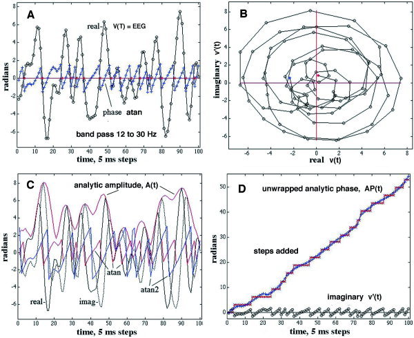
A: An example shows the EEG after it was band pass filtered (20–60 Hz). The sawtooth shows the analytic phase (AP) before unwrapping. The red asterixes show the estimated zero crossings. The open dots show the data points at 5‐msec intervals. B: The polar plot shows that the two variables define a vector with its tip at each successive point on the loops. The vector rotates counterclockwise with time, giving the cumulative increase in AP with time. The length of the vector gives the analytic amplitude (AA, red envelope in C). The AP is the angle of the vector, which is computed from the arc tangent (red sawtooth, modulo π) and (blue sawtooth, modulo 2π). C: The real part of the EEG signal is shown by the solid black curve. The imaginary part (dotted black curve) approximates its time derivative. D: The phase after unwrapping shows an increase, for which the average slope is the frequency in radians/second, The unwrapped atan phase is shown on the abscissa. The steps in phase are added at the downward zero crossings of the sawtooth.
Single EEG time series as shown in Figure 1 appeared to be tractable, but multiple time series did not. A set of 64 unwrapped AP(t) is shown in Figure 2, grouped by color into 4 subsets of 16 adjacent channels. As was usually the case, the initial AP values were distributed within ±π about zero. When temporal filtering was omitted (Fig. 2A), the mean rates of increase over the 1,250‐msec segment (250 steps at 5 msec/step) varied widely from 1 to 13 Hz. The erratic increase in AP with prominent jumps of approximately π radians was typical of that seen with colored noise. The jumps have been called “phase slip” [Pikovsky et al., 2001]. When a band pass filter was applied (12–30 Hz, Fig. 2B), the AP values increased more smoothly. However, the slopes and intercepts varied unpredictably among channels, primarily because the 64 rotating vectors did not all cross the imaginary axis simultaneously with each cycle at the mean frequency, and not all of them crossed on every cycle (Fig. 1B). This variation prevented comparisons of the AP values across channels over extended time periods.
Figure 2.
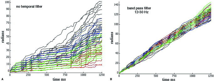
A: An example shows the analytic phase (AP) of 64 EEG signals after unwrapping without band pass filtering. The colors show groupings of 16 adjacent channels. The staircase appearance manifests “phase slip,” which is characteristic of broad‐band noisy signals. B: The AP(t) from the same EEG signals are shown with band pass filtering to minimize phase slip. The task is to find and measure phase jumps that are physiological and not noise or computational artifacts.
Importantly, the local rates of change were not so strongly affected by this variation between channels. Therefore, the temporal AP differences were calculated as time series for each channel. The spatial AP differences between channels were displayed in 3‐D graphs with magnitude of AP difference on the ordinate, time on the left abscissa, and distance (channel number) on the right abscissa (see Figs. 9, 10). The phase differences were plotted as absolute values in order to avoid hiding the negative peaks below the surface. The global mean, equivalent to the average slope and the mean frequency over the segment, was subtracted in order to remove the unregulated variance modulo π and emphasize the local deviations in instantaneous frequency about the mean frequency.
Figure 9.
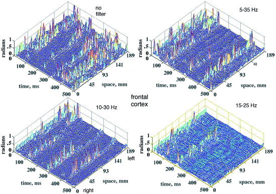
The absolute values of temporal AP differences, |AP|, are shown for 64 channels (right abscissa) of the 18.9 cm curvilinear array in a 500‐msec epoch (left abscissa). The differences are shown for 3 pass band widths with the center frequency fixed at 20 Hz for comparison with the unfiltered EEG For optimal display, the |AP| values >1 radian were clipped at 1 radian. Frontal area, eyes closed, channels numbered right to left across the midline, vertex reference. [Color figure can be viewed in the online issue, which is available at www.interscience.wiley.com.]
Figure 10.
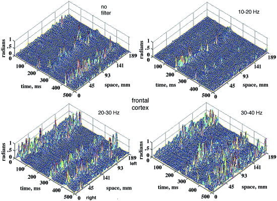
Absolute temporal |AP| differences are shown for 64 channels in the 18.9‐cm curvilinear array. They were computed in a 500‐msec segment after band pass filtering the 64 EEG with 3 center frequencies. The band width was fixed at 10 Hz for comparison of |AP| differences with no filler. Frontal area, eyes closed, 0 to 64 right to left across the midline forehead, vertex reference. [Color figure can be viewed in the online issue, which is available at www.interscience.wiley.com.]
Experience with animal data had shown that the direction of change was immaterial. Further enhancement of display was based on an empirical observation that rapid physiological changes in AP tended to occur at many locations nearly simultaneously and to be accompanied by minima of the AA on the same channels. Selective emphasis for display of the sudden changes in AP that were nearly simultaneous across multiple channels was facilitated by converting the AA to a weight, W,
| (6) |
The values of W ranged inversely from near zero for high AA to 1 for zero AA. The absolute de‐meaned AP(t) values were multiplied by W(t). This algorithm improved the detection of synchronization among the temporal AP differences by taking advantage of the information in the AA (see Fig. 14). As shown in Figure 1C, the minima in AA were largely independent of the zero crossings of the band pass filtered EEG [Freeman et al., 2003].
Figure 14.
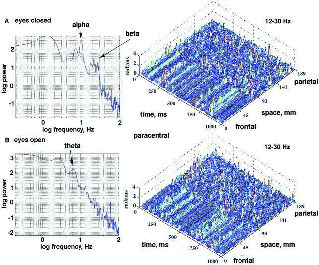
A: With eyes closed, the weighted |AP| differences were spatially correlated in stripes that repeated at intervals in the α range (cospectrum on left) across the right paracentral area anteriorly (channels 1–30) but not posteriorly (right). B: With eyes open, the spatial correlation of the clustered AP differences (CAP) persisted but repeated at a mean frequency in the θ range in accordance with the cospectrum (left). The optimal correlation was sought in the α range for both conditions. Epoch duration: 1 sec. [Color figure can be viewed in the online issue, which is available at www.interscience.wiley.com.]
The salient problem in applying the Hilbert transform to EEG was finding effective criteria for the choice of the temporal pass band. In prior studies of animal EEG, an optimal pass band was chosen by means of a behavioral criterion. The pass band was systematically varied to make tuning curves, and the settings of the upper and lower cut‐off frequencies were found at which the rates of correct classification of spatial AM patterns of EEG amplitude were highest (20–80 Hz in rabbits [Barrie et al., 1996]; 35–60 Hz in cats [Freeman et al., 2003]). The finding emerged from those studies that the correlation of AP phase differences with EEG activity in the θ ranges was also optimized [Freeman and Rogers, 2002]. In the absence of an appropriate behavioral measure in the present study, the optimal pass bands for temporal filtering before application of the Hilbert transform were found as follows. Autocorrelations were calculated for each channel averaged over channels in segments 2 sec in duration for the raw EEG and the signed temporal AP differences, and so likewise the cross‐correlation between them. The temporal PSDt of the raw EEG (Fig. 3A), the AP differences (Fig. 3B), and cospectrum (Fig. 3C) were calculated for the averages over channels. The frequency, fm, at the maximum of the power, pm, in the cospectrum was identified within the alpha (α) range (7.5–12.5 Hz, Fig. 3C) rather than the θ range, owing to the predominance of α in the human scalp EEG.
Figure 3.
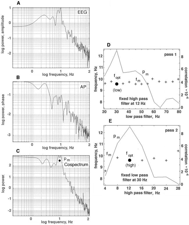
The technique for constructing tuning curves is illustrated. A: PSDt of raw EEG from frontal cortex of a subject at rest with eyes closed. B: PSDt of signed temporal AP differences after filtering the EEG in a pass band of 12–30 Hz. C: Cospectrum of raw EEG and signed AP differences for the same pass band. D: The maximal value in the cospectrum of the cross‐correlation (solid circle) was sought in the α range (7.5–12.5 Hz) as a function of the pass band. Pass 1 was to fix the high pass filter at 12 Hz and vary the low pass filter setting. E: In pass 2, the low‐pass filter was fixed and the high‐pass filter setting was stepped. The alpha frequencies at which peaks were found for each filter setting are shown by crosses; the α frequency at the peak off the cospectrum is shown by fopt (solid circle).
Control values of fm and pm were first calculated without band pass filtering. Then an optimal value of fm = fopt was found for the low pass filter in pass 1 (Fig. 3D) by fixing the high pass filter at 12 Hz and systematically stepping the low‐pass filter from 20 to 80 Hz in steps of 10 Hz. This gave a set of values for pm in the form of a tuning curve. The frequency, fopt (low), at the maximal value for pm was chosen as the cut‐off for the low‐pass filter. Next in pass 2 (Fig. 3E), the low‐pass filter was fixed at fopt (low), and the high‐pass filter was increased in steps of 4 Hz from 4 to 28 Hz. Pass 2 gave a second tuning curve of values of pm, from which the best high pass cut‐off frequency, fopt (high), was determined from the maximal pm. The same pass band was also used when maximal power shifted from the α range into the θ or δ ranges, because search outside the α range for correlations between signed AP differences and the raw EEG failed to yield clusters of large jumps in AP differences.
RESULTS
Application of the hilbert transform to scalp EEG
To illustrate the recording arrangement, a normal brain was obtained from a teaching collection. A montage was constructed of photographs taken from views perpendicular to the curved surface (Fig. 4). The radius of the brain was 7.5 cm, and the estimated thickness of the skull and scalp was 1.5 cm. The gyri appeared as light areas, and the outer aspects of the sulci appeared as dark curves, indicating the indentations in the wrinkled surface of the cortex. The circumference of the scalp of the nine subjects varied between 56 and 59 cm, giving an approximate radius of 9 cm for the head. The surface view of the cortex was up‐scaled 20% to the area of the scalp. Superimposed rows of dots on the photographic montage indicated the length, spacing, and the three locations of the curvilinear array of recording electrodes. The EEG signals and EEG deliberately contaminated by EMG recorded from the linear scalp array were unremarkable (Fig. 5).
Figure 4.
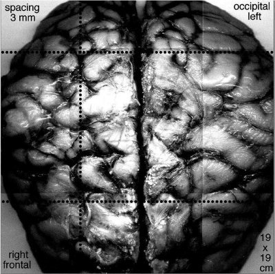
A montage of photographs shows the surface of a human brain specimen from a teaching collection. The light areas are gyri, and the dark lines are sulci. The scale has been expanded 20% from the radius of the brain, 7.5 cm, to the radius of the scalp, 9.0 cm to visualize the projection of the gyri onto the scalp. The rows of dots show the three locations of the 64×1 array of scalp electrodes: frontal, paracentral, and occipital. Adapted from Freeman et al. [ 2003].
Figure 5.
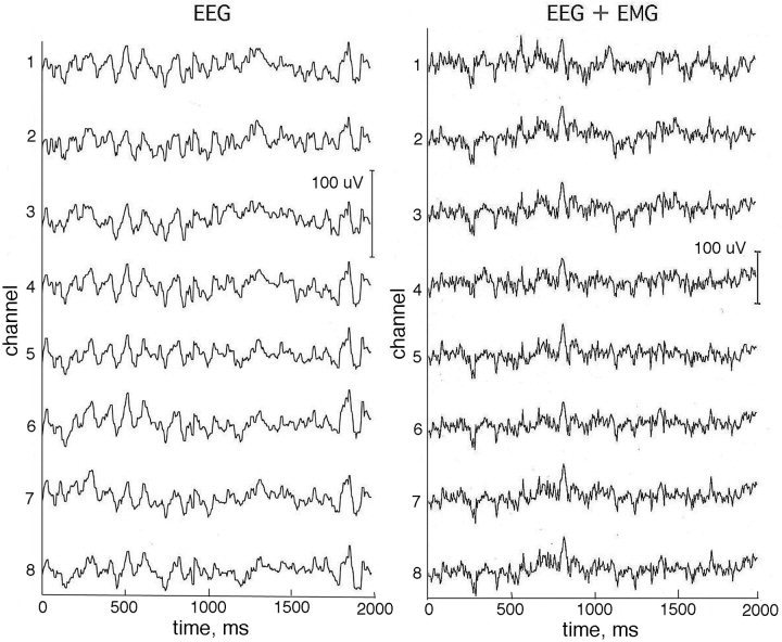
A contiguous subset of 8 out of 64 EEG traces from the paracentral scalp of an alert subject with eyes closed, at rest (left) and while inducing a modest level of EMG (right) by tensing the scalp muscles. Reference: ipsilateral mastoid.
Band pass filtering gave oscillations having fairly regularly spaced peaks and zero crossings. The AP appeared as a sawtooth time series (Fig. 1A). Unwrapping gave a ramp function (Fig. 1D) with minor irregularities and occasional dips (negative temporal AP differences). The instantaneous amplitudes of the EEG before and after the Hilbert transform at each digitizing step determined a point in the complex plane, which specified the tip of a vector extending from the origin at zero amplitude (Fig. 1B). The analytic amplitude (AA) was given by the length of the vector (the enveloping red curve in Fig. 1C) from equation (4). The analytic phase (AP) was given by the angle between the vector and the real axis in B, which was evaluated with equation (5). The vector rotated counterclockwise with successive time points, thereby tracing a loop with each cycle. Usually the loops went around the origin and enclosed it, but, as shown in this example, smaller loops might fail to circumscribe it. A short fall in a loop caused a brief period of negative AP differences (Fig. 1B). In Figure 1C, the solid black curve showed the real part of the Hilbert transform, which was identical to the EEG. The dotted black curve showed the imaginary part, which approximated the time derivative of the EEG. The two sawtooth functions in C compared the AP values derived using the arc tangent modulo π (atan) and the arc tangent modulo 2π (atan2). The atan function was found to have fewer outlying phase values than the atan2 function, so it was used routinely.
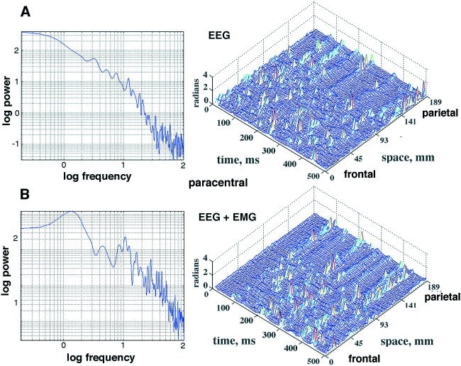
Derivation of PSD and use of band pass filters
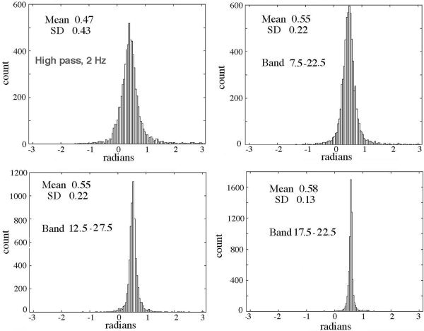
The temporal power spectral densities (PSDt) of the EEG and AP (Fig. 3) both showed linear decrease in log power with increasing log frequency, the “1/f” form, but with departures due to local spectral peaks in varying ranges [Freeman et al., 2003]. The Hilbert transform increased relative power in the AA at low frequencies and increased it at high frequencies. The amplitude histograms of the EEG were well approximated by the Gaussian function [Freeman, 1975]. Histograms of the AA resembled the F‐distribution, as expected to describe variances and covariances, extending from zero to a peak near 1 standard deviation (SD) and a long tail with high values. The effects of the band pass filters on the distributions of sequential AP differences were examined in two ways. First, the center frequency of the pass band was fixed at 40 Hz, and the pass band was changed in steps of ±5 Hz from ±2.5 to ±12.5 Hz for comparison with high pass filtering at 2 Hz (Fig. 6). The distributions were leptokurtic with high central peaks. The long tails ranged slightly beyond ±π for the atan function especially for the unfiltered EEG. For comparison, the step size of 5 msec would give an AP difference of ±π/2 radians at 52 Hz and ±0.8 radians at 14 Hz. The filtered data showed progressive diminution of the SD of the distributions with decreasing band width (Fig. 7, left). The “normal” SD for a Gaussian density distribution fitted to the center peak (omitting the tails as outliers) averaged 0.6 of the actual SD. The mean AP difference was relatively independent of band width. Second, the band width was fixed at ±5 Hz, and the center frequency was stepped at 10‐Hz intervals. The mean value of sequential AP differences co‐varied with band width, but the SD did not (Fig. 7, right).
Figure 6.
The distributions of sequential AP differences after temporal filtering of the EEG before applying the Hilbert transform are shown for band widths that all had the same center frequency of 40 Hz.
Figure 7.
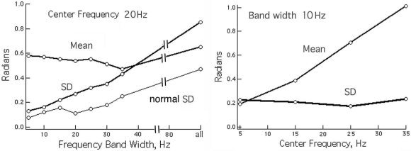
The relations are shown between the mean and SD of the sequential AP differences and variation in the band with or center frequency. The “normal” SD was derived by fitting a Gaussian curve to the center peak, omitting the tails. Left: The center frequency was fixed, and the band width was varied. Right: The band width was fixed, and the center frequency was varied.
Spatial clustering of synchronous temporal phase jumps across channels
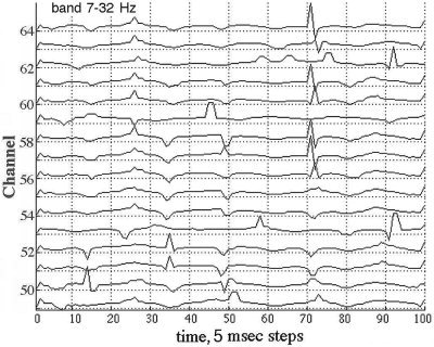
The relatively small number of large sequential AP differences tended to occur in spatiotemporal clusters on multiple adjacent channels within 2 to 4 samples (10 to 20 msec at the 5‐msec digitizing interval). Figure 8 shows a typical example of the sequential differences for 16 signals from adjacent electrodes. The maximal differences were either positive or negative in the same time frame, sometimes appearing biphasic (steps 70–74, channels 56–64 in Fig. 8), which was not unusual for the Hilbert transform, especially when the segment length was not a power of 2. The direction of change in AP was less important than the timing, so the absolute |AP| differences were plotted for the entire array as time functions in 2‐D, after subtracting the global means (Fig. 6). An example from the frontal area of a subject with eyes closed and high α activity shows that the |AP| jumps were often synchronous across part or all of the array (Fig. 9). The locations in time and space of the synchronized AP jumps varied depending on the width of the pass band, and on the presence or absence of α or θ peaks in the PSDt, here with prominent α. Figure 10 shows the spatiotemporal clusters from another subject, also recorded over the frontal area with eyes closed but with no periodic α activity and minimal θ. The times at which spatiotemporal clusters were revealed tended to vary with the center frequency of the narrow pass band. These findings held also for the paracentral and occipital areas in the presence or absence of periodic α or θ or both.
Figure 8.
A representative set of EEG from 16 of 64 consecutive channels shows sequential differences, AP(t) − AP(t−1), at the digitizing step of 5 msec after filtering in the pass band of 12–30 Hz. The problem is to distinguish the jumps that arise from cortical dynamics from those due to phase slip owing to noise, nonlinearities, and numerical artifacts.
Using AA differences to enhance visualization of AP differences
Correlation of the AA(t) and AP(t) showed that wide excursions in the time derivative of the AP in either direction often accompanied substantial decreases in AA on the same channels. The spatial ensemble average of the fluctuations in AA over the 64 channels in a 1.25‐sec epoch are shown by the blue curve Figure 11A. The standard deviation (SD) of the spatial AA differences at each time step (red curve) was relatively constant despite the wide fluctuations in the mean on each channel. The vertical bars were drawn where the average AA fell below an arbitrary threshold of 1.75. The absolute values of AP were taken after subtraction of the mean corresponding to the frequency. The average absolute |AP| after demeaning (Fig. 11B, blue curve) and its SD over the 64 channels (red curve) co‐varied closely. The peak |AP| values tended to occur at the minima of AA, as shown by the vertical bars extended from frame A. The distribution of the 250 pairs of AA and |AP| in a representative EEG segment lasting 1.25 sec (Fig. 12A) confirmed the inverse relation.
Figure 11.
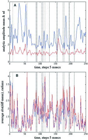
A: The average (blue/black curve) and SD (red/gray curve) were calculated for the AA(t) values from the 64 EEG in a 1.25‐sec epoch. The vertical bars indicate times at which the average AA fell below an arbitrary threshold of 1.75. N = 250. B: The average (blue/black curve) and SD (red/gray curve) of the absolute |AP| sequential differences showed peaks tending to occur at times when the average AA approached a minimum. N = 16,000. Paracentral area, eyes closed, EEG pass band 15–55 Hz. [Color figure can be viewed in the online issue, which is available at www.interscience.wiley.com.]
Figure 12.
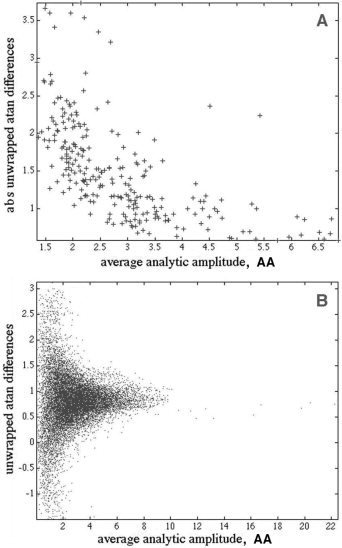
The relations among AA, AP, and W were examined graphically. A: The absolute temporal differences |AP(t) − AP(t−1)| were averaged over the 64 channels in a segment 1.25‐sec long sampled at 2‐msec intervals (N = 250) and plotted against the AA(t) averaged across channels at the same times. An inverse relation was found between AA and |AP|. B: Signed AP temporal differences were plotted against AA amplitudes for all 64 channels and time points (N = 16,000), showing the preponderance of large deviations in signed AP from the mean with low values of AA. Paracentral area, eyes closed, EEG pass band 15–55 Hz.
The distribution of the average values of |AP| is plotted as a function of average values of AA in Figure 12A, showing the tendency for low AA to be accompanied by high |AP|. The distribution of the signed AP differences from the 64 channels (Fig. 12B) prior to de‐meaning shows the mean frequency as the positive offset. Most of the AP differences were positive. The small number of negative and unusually high positive values were paired with low values of AA (averaged across the pair of AA values used to compute the AP difference), although the majority of minima in the AA were not accompanied by concomitant extremata in the AP differences.
The effect of weighting the |AP| differences by W is shown in Figure 13. Without weighting, the sizes of the synchronized changes in differences of |AP| from the mean were both upward and downward though always positive. With weighting, the dips were reversed to upward deflections, and the plateaus between jumps were smoothed.
Figure 13.
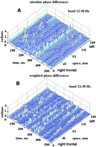
A: The spatiotemporal clustering of absolute |AP| differences on 64 channels in a 5‐sec ecepoch showed both dips and peaks tending to synchronize over the whole array, but with interhemispheric offsets. B: The absolute |AP| differences weighted by equation (6) were all upward, with some sharpening of clustering. Frontal area, channel numbering right to left, eyes closed, pass band 12–30 Hz. For the PSDt, see Figure 3A. [Color figure can be viewed in the online issue, which is available at www.interscience.wiley.com.]
Using tuning curves to minimize effects of phase slip
Figure 3 showed the spectrum of the autocorrelation of the EEG (Fig. 3A) and the spectrum of the autocorrelation of the signed AP differences (Fig. 3B). The peak in the α range of the cospectrum of the cross‐correlation averaged over all 64 channels (Fig. 3C) was found to be maximal with the pass band prior to the Hilbert transform set at fopt (low) = 12 (Fig. 3D) and fopt (high) = 30 Hz (Fig. 3E). The mean and SD for the α frequency at the peaks of correlation (indicated by solid circles) were 8.93 ± 0.67 Hz, with no significant differences between occipital, paracentral and frontal areas. This pass band, 12–30 Hz, for optimizing the clusters of AP changes (CAP) synchronized with α was found in all subjects. The synchrony of the CAP jumps was again clarified by weighting the absolute time differences of the AP across the array with equation (6). In an example (Fig. 14) from the paracentral area a subject at rest with eyes closed (Fig. 14A) was asked to open the eyes (Fig. 14B). A peak in the α range of the autospectrum and cospectrum vanished, while another appeared in the θ range. The CAP in this case were found over the frontal area and not over the parietal area, and the spatial distribution of CAP persisted at the lower recurrence rate. In another example (Fig. 15), from the paracentral area the subject at rest with eyes closed was asked to tense the scalp muscles. There was no α peak in the PSDt of the EEG or the cospectrum (Fig. 15, left). With onset of EMG, a weak α peak emerged in the cospectrum, and the stripes of CAP persisted in the parietal area. Despite the increase in power in the β and γ ranges contributed by the EMG, as documented in detail in a companion report [Freeman et al., 2003], the synchronized clusters of CAP were clearly visible (Fig. 15B) over the posterior third of the array.
Figure 15.
A: A subject at rest with eyes closed gave spatially ordered peaks in CAP in the paracentral area posteriorly (right) but with no alpha in the EEG or alpha peak in the cospectrum (left). B: With deliberate induction of EMG, the amplitude of the signals increased across the entire spectrum (left). CAP persisted in the same parietal area (right). Epoch duration: 0.5 sec. [Color figure can be viewed in the online issue, which is available at www.interscience.wiley.com.]
These examples illustrated the way in which the curvilinear array could be used to estimate phase velocity. The variation of the AP jumps from the mean time of occurrence in the CAP stripes in some instances was within the 5‐msec digitizing step over the array length of 18.9 cm independently of the orientation of the array. Whatever the delay over the array, the phase velocity would have had to exceed 40 m/sec in the direction parallel to the array, and 20 m/sec in directions ±60 degrees from the array. For lesser velocities, the peaks in the CAP would have lain diagonal to the right abscissa in the mesh plot, as in fact was occasionally noted in short segments.
Other manipulations of the AP differences prior to display
The effects on the CAP of three types of randomization were examined (Fig. 16). A data set was processed from the occipital cortex of a subject at rest with eyes closed that showed CAP stripes bilaterally (Fig. 16A) with temporal filtering at 12–30 Hz. Randomization of the channels (Fig. 16B) by reordering them with a table of random numbers introduced noise without significant loss of the CAP. Surrogate data were generated by taking the FFT of the filtered EEG on each channel, randomizing the phase values, and taking the inverse FFT, thereby keeping the power and second order statistics intact. This procedure (Fig. 16C) diminished but did not abolish the CAP. Shuffling was done by using a table of random numbers to select at random a time point in each EEG and translating the later segment to precede the earlier segment (Fig. 16D). This re‐ordering of the sequences on the channels destroyed the CAP.
Figure 16.
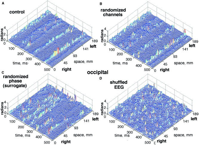
Three types of statistical control are illustrated. A: The control mesh shows CAP stripes extending across occipital areas bilaterally with the pass band set at 12–30 Hz. B: The channel order was randomized. C: The EEG signals were transformed by the FFT, the phase values were randomized, and the inverse FFT was taken to generate the surrogate signals. D: The EEG were shuffled by segmenting the signal on each channel at a time point chosen at random and translating the latter portion from after the point to before. [Color figure can be viewed in the online issue, which is available at www.interscience.wiley.com.]
Spatial filtering of the EEG applied before temporal filtering further clarified the CAP. The choice of low‐pass filter setting was based on the 1‐D spatial PSDx of the 64 raw EEG amplitudes, averaged over 1,000 time points (500 steps) [Freeman et al., 2003]. Examples of PSDx from four subjects are shown in Figure 17A from the frontal cortex with no temporal filtering. Typically, the rate of decrease in log power with log frequency did not conform to 1/f for scalp EEG as it did for intracranial EEG [Freeman et al., 2000], and small peaks figured persistently in the range of 0.1 to 0.5 c/cm. For comparison with the anatomy, the photographic montage (Fig. 4) was digitized at a grain of 1 mm, and the 2‐D FFT was used to calculate the spatial spectrum of the image of the cortical surface (Fig. 17B). The basic form of the spatial spectrum of the montage was 1/fα, where α = −1.7, with a broad peak in the range of 0.1 to 0.5 c/cm, corresponding to the typical length (3–5 cm) and width (1 cm) of human gyri. A low‐pass spatial filter was set at 1.05 c/cm to smooth variations near the Nyquist frequency (1.67 c/cm), at 0.40 c/cm near the width of gyri, and at 0.167 c/cm near the length of gyri.
Figure 17.
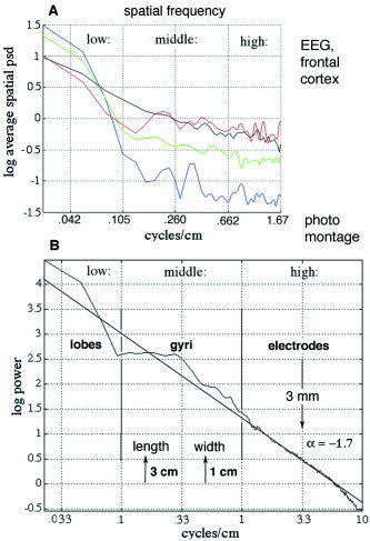
A: Examples are shown of the spatial spectra (PSDX) from the frontal cortex of four subjects at rest with eyes closed. B: The 2‐D FFT was taken of the photograph in Figure 4 digitized at 1‐mm steps to get the spatial power spectral density, PSDX. The central peak corresponded to the typical length (3 cm) and width (1 cm) of gyri, and to peaks in the PSDX of the EEGs. The spectral form was 1/fα, where α = −1.7. Adapted from Freeman et al. [ 2003]. [Color figure can be viewed in the online issue, which is available at www.interscience.wiley.com.]
The effect of spatial filtering is shown by the example in Figure 18. A control with no spatial filter is shown from the occipital cortex of another subject (Fig. 18A). The two hemispheres were not synchronized. The array length of 18.9 cm and spacing of .3 cm set a low‐frequency bound of 0.053 c/cm and an upper Nyquist bound of 1.67 c/cm. A low‐pass filter was applied to the EEG data before temporal band pass filtering with a set point at 1.05 c/cm (Fig. 18B), then at 0.4 c/cm (Fig. 18C) and 0.167 c/cm (Fig. 18D). The clarity of the CAP was progressively improved. The effect of a high‐pass filter on the CAP from the frontal cortex (Fig. 4, lower row of dots) of a subject at rest with eyes closed is shown in Figure 19. Compared with the control (Fig. 19A), the filter set at 0.1 c/cm virtually abolished the CAP from the mesh plot (Fig. 19C). Re‐referencing by subtracting the spatial ensemble average (fig. 19B) obscured the CAP and at the same time diminished the α peak in temporal spectra from the frontal area [Freeman et al., 2003]. This decrease did not occur with re‐referencing in spectra and mesh plots from the paracentral and occipital areas. Shifting the temporal pass band from 12–30 to 20–40 Hz (Fig. 19D) or yet higher spectral ranges preserved the CAP stripes but shifted them to new time locations. The use of low pass spatial filtering enables increased visualization of the phase jumps of the high frequency oscillations, extending the range from β well into the γ activity (Figure 20). This effect introduced a new dimension to the study of CAP, which was too complex to be explored in this introductory study.
Figure 18.
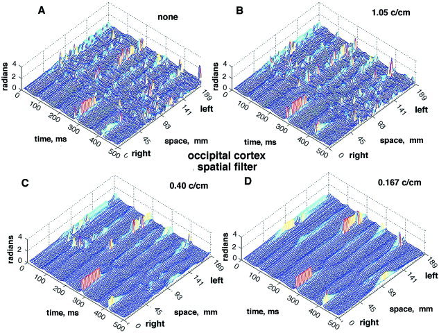
The effects on the CAP are illustrated of applying a low‐pass spatial filter to the 64 EEG signals after global de‐meaning and prior to temporal band pass filtering. A: No filter. B: 1.05 c/cm (wave number = 6.6 radians/cm, wave length = 9.5 mm). C: Filter at 0.4 c/cm (wave length = 25 mm). D: Filter at 0.167 c/cm (wave length = 60 mm).
Figure 19.
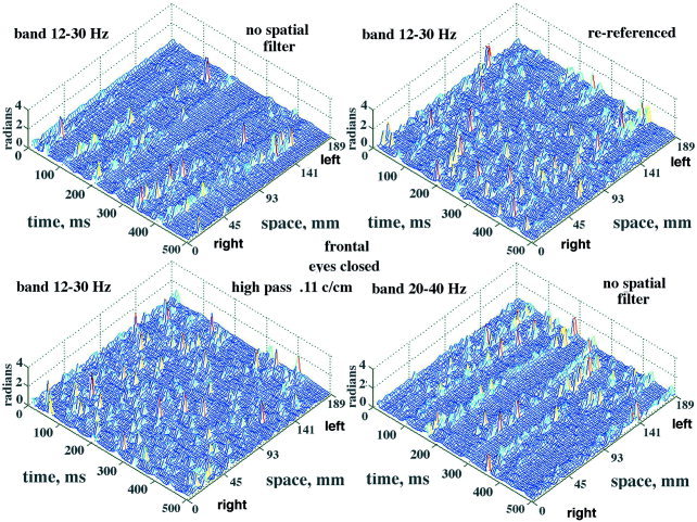
Three types of data manipulation are illustrated. A: The EEG of a subject at rest with eyes closed yielded CAP in the frontal area bilaterally with some dissociation between locations. The optimized pass band was 12–30 Hz. B: The CAP disappeared on re‐referencing by subtraction of the spatial ensemble average. C: A high‐pass spatial filter set at 0.042 c/cm (wave length exceeding the length of the array) also suppressed the CAP. D: Shifting the pass band to 20–40 Hz retained the CAP but shifted the stripes to different times and locations. Epoch duration: 0.5 sec. [Color figure can be viewed in the online issue, which is available at www.interscience.wiley.com.]
Figure 20.
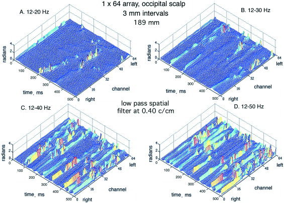
The subject was asked to remain motionless with eyes closed and sustain mild contraction of the scalp muscles to generate EMG less than twice the amplitude of the resting EEG. The pass band of the temporal filter was increased in steps from 12–20 Hz to 12–50 Hz. Each step revealed further structural detail in the CAP differences. The peak of the cospectrum was in the theta range. When the subject terminated the deliberate EMG and returned to rest, the peak in the cospectrum returned to the α range.
DISCUSSION
Advantages and limitations of the hilbert transform
The rationale for adapting the Hilbert transform to analysis of scalp EEG was based on the hypothesis that abrupt changes in cortical states occurred stepwise at rates in the δ, θ, and α ranges [Freeman and Rogers, 2000]. Such changes were seen in EEG recorded in animals intracranially [Freeman and Barrie, 2000; Freeman, 2003b]. From estimates of their spatial distributions in sensory cortices, the stepwise changes appeared to be synchronized over distances that might make it possible to detect them in scalp EEG, if indeed these or similar abrupt changes occur in human cortex. The changes in animals had the form of synchronized modulations of amplitude and frequency at a common phase of the ongoing oscillations of EEG recorded from multiple locations. Owing to its high temporal resolution (approaching the digitizing rate), the Hilbert transform was deemed to be more likely than Fourier‐based procedures to enable precise temporal localization of the abrupt changes, because its temporal resolution approached that off the digitizing rate, although tests with a cosine having a simulated abrupt phase shift showed that the AP difference was spread over 2–4 steps, depending on the magnitude of the shift. An additional advantage in the present study was the precise spatial localization afforded by the high‐density array of electrodes, which provided the best means for discerning physiological jumps from phase slip by virtue of spatial clustering.
The main difficulty in using the Hilbert transform arises from the intrinsic discontinuities in the AP function that necessitate unwrapping. As seen in Figure 1A, the amplitude and rate of change of an EEG signal can be represented by a vector, for which the change with time is in its length and its rotation about the origin of the complex plane, usually counterclockwise. The procedure allows the display of the EEG amplitude and phase as independent variables. The rotation gives a ramp‐like increase in phase with time, but with breaks when the vector crosses the imaginary axis (re‐setting the phase by −π) or the negative real axis (re‐setting the phase by −2π). The difficulty of the correction by unwrapping to give a continuous ramp lies in predicting the size of the phase increment across the break. The step in AP is easy to add when signals are periodic, but the modification can be very difficult with the noisy, aperiodic signals of EEG [Pikovsky et al., 2001; Tass et al, 1999], especially when the EEG dithers above or below zero without crossing. In the case of unfiltered EEG having the 1/f form of PSD, the AP has the appearance of a random walk or a Markov process known as “phase slip.” The difficulty becomes most obvious in displays of the signals from multiple channels in which the time series are spatially coherent (Fig. 5), but in which the AP(t) differences diverge in staircase form with jumps predominantly near π radians (Fig. 2).
On the one hand, in both theory and practice [Freeman and Rogers, 2000] an increment in AP(t) signifying a physiological change in cortical state can be negative or positive (backward or excess forward rotation) or so small as to be indistinguishable from the average increment. Especially if the state change occurs as the vector crosses an axis of the complex plane, it may be missed altogether. On the other hand, there are several ways in which unusual increments can appear in EEG from arrays of electrodes, in addition to thermal noise or movement artifacts on one or more channels. The beating of two periodic components with nearly the same frequency can give a phase jump when the sum of amplitudes goes through zero. A high‐frequency component riding on a low‐frequency component can cause a failure of an expected zero crossing. This may be exemplified in Figure 1B, where loops of the trajectory of the vector sometimes fail to enclose the origin, and the AP differences are briefly negative (Fig. 12B). If the noise or the mixed frequency components were to occur at the reference electrode with referential recording, then increments of unusual size would appear on most or all of the channels. Hence, the Hilbert transform can miss state changes, and it can generate false reports of state changes.
One recourse is to narrow the pass band of the temporal filter so as to reduce phase slip. Studies by Le Van Quyen et al. [ 2001] and Quiroga et al. [ 2002] have shown that measurements of phase by the FFT and the Hilbert transform with very narrow pass bands give nearly equal values, showing their equivalence under this constraint. However, the temporal resolution offered by the Hilbert transform is compromised by narrow band filtering, and the opportunity to track nonlinear frequency modulation in the form of phase modulation, giving temporal coherence to chaotic time series, is lost. Therefore, some band pass filtering is necessary, but not to the point of significant impairment in temporal resolution.
Determination of optimal time windows and spectral pass bands
The further hypothesis emerged from animal studies that there are two main classes of EEG oscillations that are required for cortical states and state changes: low gating frequencies in the δ and θ ranges, and high carrier frequencies in the β and γ ranges. Sensory cortices in rabbits and cats with arrays of electrodes surgically implanted subdurally sustained wave packets, which were brief epochs of spatially coherent oscillation in the β and γ ranges. The wave packets revealed spatial phase modulation (PM) of the carrier wave in the form of a cone. The spatial phase gradient in radians/mm (the slope of the PM cone), when it was converted to m/sec with the center frequency of the carrier wave, conformed to the range of conduction velocities of intracortical axons running parallel to the pial surface [see references in Freeman and Baird, 1987; Freeman and Barrie, 2000; Freeman and Burke, 2003]. The time period required for a phase change was estimated to range from 3–7 msec, and the duration of wave packets was estimated to range from 76–101 msec. The recurrence rate averaged 4.01 ± 1.53 Hz, so the time interval between wave packets ranged from 80–324 msec [Freeman, 2003b].
These numerical estimates supported the predictions that jumps in phase of unusual size with the Hilbert transform in the time domain would be synchronous in local areas of cortex within 3–7 msec, and that the distribution of increments in the same state change would include both directions (forward or backward, lead or lag) and at some locations no detectable AP difference [Freeman and Rogers, 2002]. The estimates provided an essential guideline for designing synchronization indices by applying an 80‐msec moving window to the data for de‐meaning and calculation of Shannon entropy. In the spatial domain, most wave packets in animal studies were 1 to 3 cm in diameter with a mode of 1.5 cm, so that if they occurred in that size range in human cortex, they would be detectable at the scalp in signals from only 3 to 9 contiguous electrodes with 3‐mm spacing. In a preceding report on the spatial and temporal spectra of EEG [Freeman et al., 2003], the spectral pattern was described of a peak in the spatial PSDX located in the range of 0.11–.26 c/cm, which was broadly distributed in the temporal PSDt. This pattern was described as the signature of a temporal impulse with a spatial period of 4–9 cm. The stripes that manifested the CAP could account for the temporal impulse. It was inferred that if phase cones and wave packets existed in human cortex, the diameters of the PM cones would be in the range of 2.0–4.5 cm, or about twice the diameter of the phase cones in rabbits. That size range served to predict that CAP would be found to occur on 6 to 15 contiguous electrodes at 3‐mm spacing. The CAP were found in that range, but also in larger sizes up to the entire array, with less temporal spread than had been expected. This discrepancy suggested that the phase changes manifested in the more widespread CAP stripes in scalp EEG might differ from those involved in forming wave packets in local areas of cortex.
Developments in techniques to search for AP differences
The definition and description of wave packets were based in the behavioral correlation of the AM and PM patterns with behavior. The present preliminary study lacked an extensive behavioral database. The technical problems to be solved were to devise optimal criteria by which to distinguish physiological phase jumps from those due to noise and artifacts, or to meaningless neural events resembling random avalanches in sand piles [Bak et al., 1987]. Six procedures for interim optimization were examined here.
Unwrapping
First, four methods were explored for unwrapping: the MATLAB algorithm of adding a fixed correction at each branch point in time; an algorithm for locating zero crossings as an indicator of the need for a correction [Freeman and Rogers, 2002], estimation of when to add the required 2π offset with the atan2 algorithm; and estimation of when to add π with the atan algorithm. Of these, the fourth procedure gave the smoothest ramp with the lowest number of outliers.
Band pass temporal filtering
Second, despite the 1/f form of the spectra of EEG and AA, narrow band pass filters were applied to the EEG prior to application of the Hilbert transform in search of the pass band of an optimal carrier frequency that might most clearly manifest state changes. In animal studies, the pass band was evaluated by optimizing the classification of spatial AM patterns with respect to CS, giving species differences between cat and rabbit [Freeman, 2000a]. Here, the pass band was varied in search of CAP. As predicted, the mean of the distributions of AP differences depended on the center frequency of the pass band, and the variance depended on the band width. Spatial stripes of CAP were found in all of the files in at least some epochs, with varying spatial extents ranging from a few channels to the entire array. As expected, both forward and backward directions of AP differences across the array appeared within the same brief time periods. The clarity of the appearance of CAP was improved by display of the absolute values of the AP differences. Clarity improved with pass bands down to 20 Hz but was inadequate with those <10 Hz. This result was consistent with the finding that CAP occurred in different pass bands at different locations in time, indicating that they can coexist in the data, much as multiple phase cones were found to overlap in animal studies.
However, commonly within the same file there appeared stripes of CAP at differing times in different pass bands, particularly contrasting the β and low γ pass bands, so that multiple interleaved CAP were implied. This finding further raised the complex question, not yet answered, how subtle interactions between the narrow filters and the broad 1/f spectral distributions of the β and γ activity might give the appearance of distinctive, temporally interleaved markers for sequential state changes, or stages in the induction of each state change within a longer time window. Answers may require data taken at digitizing intervals of 1 or 2 msec instead of 5 msec as in the present study.
Use of minima in AA to clarify CAP
Third, unusually large increments in AP(t) differences tended to be accompanied by low values of AA, suggesting that a characteristic of cortical state changes was temporal amplitude modulation, by which at the AA tended to a minimum at the moment of a state change. This finding was exploited by converting the AA(t) values from the filtered EEG signal to a weighting factor, W in equation (6), which approached zero for large AA and unity for small AA. Each AP difference was multiplied by the weight so as to diminish it between state changes and enhance it during state changes. This procedure enhanced the clarity of visual displays of the CAP. However, the variance of the relation between AA and AP was high, with numerous unexplained discrepancies in all directions, and, owing to the broad spatial distributions of mixed frequency components, the algorithm could not unequivocally distinguish AP jumps signifying state changes from those due to shifting low frequency base lines and the beats of oscillations in adjacent frequency bands.
Tuning curves to optimize the temporal pass band
Fourth, note was taken of the finding in files from occipital and paracentral areas that the interval between stripes was within the range of α wave durations. This finding was exploited by cross‐correlating the unfiltered EEG with the AP differences after band pass filtering, computing the cospectrum, and finding the maximal peak in the α range, here 7.5 to 12.5 Hz. The procedure was repeated while systematically varying the upper and lower pass bands. The resulting tuning curves further enhanced the clarity of the CAP stripes across the array. Tuning curves were also used extensively in EEG studies of spatial AM patterns [Barrie et al., 1996; Freeman et al., 2003] and PM patterns [Freeman, 2003b].
However, the optimized pass band for the human AP(t) differences was in the β range, not in the γ range as had been predicted from the animal studies. The method for optimization of the pass band did not give sharp tuning curves in the absence of a detectable peak in the α range, and it was of little value for maximal power in the δ range, <3 Hz. There were too few files with PSDt peaks in the θ and γ ranges to support systematic investigation of the effects of varying the search range for the gating frequency outside the α range. Mesh plots of AP differences within the optimal β band of 12 to 30 Hz from files with no α activity revealed stripes of CAP recurring aperiodically, indicating that AP stripes were not dependent on detectable α (Fig. 19A), as were the tuning curves. Other stripes recurring at α rates were equally prominent after temporal filtering to enhance the low γ band, with or without α peaks in the PSDt from unfiltered EEG (Fig. 10D).
Spatial low pass filtering
Fifth, the measurement of phase cones in EEG from subdural recording in animals was facilitated by low‐pass spatial filtering at 0.29 c/cm [Freeman and Barrie, 2000], and they were removed from the data by high pass filtering at 0.15 c/cm [Freeman and Baird, 1987]. The results here replicated both the deleterious effect of high‐pass spatial filtering on the visualization of recurring stripes of CAP and the clarification of low‐pass filtering. Evaluation of the utility of spatial filtering was facilitated by over‐sampling with a curvilinear array, with electrodes spaced 3 times more closely than the typical width of underlying gyri, conforming to the practical Nyquist criterion [Barlow, 1993]. The combination of oversampling and smoothing appears to be optimal for spatial textural analysis [Freeman et al., 2003a, 2003b]. However, the CAP phenomenon should also be accessible by means of the standard 10–20 clinical montage.
Comparison of resting state with intentional action
Sixth, the determination of an optimal pass band for application of the Hilbert transform to data from animals was based on a behavioral assay: the optimization of the classification of spatial AM patterns with respect to conditioned stimuli by varying the temporal band pass filter. The carrier waves of the wave packets were found in the β and γ ranges of 20 to 80 Hz in rabbits [Barrie et al., 1996] and 35–60 Hz in cats [Gaál and Freeman, 1998]. In the present study, the two behaviors were opening the eyes and intentionally adding EMG. Both actions were accompanied by tendencies of a temporal spectral peak to drop from the α range and sometimes for another to appear in the θ range. The spatial patterns of CAP stripes appeared to change in location and in detail. However, pattern analysis has not yet been undertaken. The clear visualization of CAP stripes in epochs when the EEG was overlain by EMG is strong evidence that the CAP are accessible in scalp EEG despite EMG. They are not wholly artifacts of data processing of aperiodic oscillations, because the PSDt and PSDX of EMG are broad and tend to be flat rather than 1/f [Freeman et al., 2003], indicating that EMG resembles white or colored noise and lacks the scaling properties of the EEG.
More study is needed, in particular to address the question whether the CAP stripes signify either idling of cortex, which is thought to occur during the relaxed awareness of traditional α states, or sequences of cognitive states, as manifested in EEG from intracranial electrode arrays in animals that yield AM patterns containing behaviorally related information, and that recur at rates in the θ and δ ranges. The α peaks clearly facilitated the construction of tuning curves for band pass optimization, but once that band was identified, the CAP stripes were found in the absence of an α peak. Furthermore, the CAP stripes typically were aperiodic, suggesting that the disappearance of an α peak manifests not “de‐synchronizing” but “de‐periodicizing,” meaning that activity persists in the α range but so erratically as to broaden the peak beyond recognition. From animal studies, it appears that the best way to search the data for cognitive correlates is to extract the AM patterns from the EEG, map them in high dimensional state space, and classify them with respect to reproducible behaviors of subjects [Freeman and Grajski, 1987]. A property of the AM patterns that facilitates classification is the fact the information content in the intracranial AM patterns is uniformly distributed over the channels. No channel is any more or less important than any other channel, as shown by deletion of randomly selected channels [Fig 7 in Freeman and Baird, 1987; Fig 13 in Barrie et al., 1996; Fig 3 in Ohl et al., 2001]. This equivalence means that EEG data from sulci that is missing from scalp recordings may have no greater value for pattern classification than that from gyri that readily contributes to the scalp EEG, diminishing the need for intracranial recording. Animal studies indicate further that spatiotemporal patterns of AP have no utility for classification of EEG spatiotemporal patterns with respect to behavior, beyond serving as spatiotemporal markers of plateaus of AP(t) differences in which to search for AA(t) patterns.
Establishment of the behavioral correlates of changes in AA and AP will be necessary to answer the following question. Is the concentration in jumps of AP at times when the AA is low owing to loss of precision in the digitized data at low amplitudes, or can it be ascribed to a tendency for AA to go to a minimum at moments of phase change? No amount of signal processing can answer this question without reference to the possible cognitive content of the EEG.
Neural mechanisms of synchronization of jumps in CAP
The neural mechanisms of the CAP stripes remain open to speculation. The CAP stripes are not due to activity at the reference electrode or to deep‐lying generators, despite the adverse effects of high‐pass spatial filtering and re‐referencing, for the following reasons. The stripes sometimes occupy the entire array (Figs. 10, 13, and 16) but more often only a portion (Figs. 14, 15, and 18), and the signed AP differences persist locally within the stripes, all with the same reference lead. This conclusion must be tempered by the realization that some as yet undetected sources of variation may exist in the multiple steps of data processing. The widespread synchrony may indicate the actions of neural mechanisms of global coordination, for which analysis of the timing will require a higher digitizing rate than the 200 Hz used here. An obvious candidate for coordination in and between hemispheres is control by thalamocortical projections [Hoppenstaedt and Izhkevich, 1998; Steriade, 2000; Taylor, 1997]. The precision of timing might be consistent with the central location of the thalamus, making it roughly equidistant from the cortical areas underlying the locations of the array in this study. The low sampling rate of 200 Hz cannot support exploration, though it suffices to show that the AP differences do not occur as diagonal stripes, as might be expected from observations on phase lags in α activity across the vertex with magnetoencephalogram [Joliot et al., 1994], particularly with paracentral placements running anteroposteriorly.
The “zero phase lag” relations in the γ range that are often reported in the literature present an even more difficult problem. A nominal limiting velocity of 10 m/sec in cortex would suggest a maximal delay of 20 msec across the curvilinear array, corresponding to 4 digitizing time steps of 5 msec, which should have been commensurate with the temporal spread of CAP in this study, but a delay of 20 msec equals wave duration in the upper γ range, and that is not compatible with a high degree of synchrony in the γ range as widely reported [e.g., Haig, et al., 2000; Singer and Gray, 1995; Varela et al., 2001] and seen in spatial and temporal spectra from scalp EEG [Freeman et al., 2003].
Self‐organized criticality and anomalous dispersion
An alternative theory by which to investigate cortical state changes is self‐organized criticality [Bak et al., 1987], in which the gyri, lobes, hemispheres, and forebrain can be conceived as maintaining themselves in metastable states close to instability. The applicability of this theory to cortex is suggested by the 1/f form of the temporal and spatial spectra from the EEG, indicating power law scaling [Freeman et al., 2003; Hwa and Ferree, 2002; Linkenkaer‐Hansen et al., 2000]. The cortex is seething with changes in state occurring simultaneously at all scales of time and space, ranging from those of single neurons through the mesoscopic states of wave packets to the entire forebrain. The possibility is that, while most of the state changes are local in time and space, some of them occasionally cascade into collections of coordinated wave packets and then into hemisphere‐wide synchronized jumps in state, as revealed by CAP differences. The value of scalp recording emerges from the smoothing by the intervening soft and hard tissues, which attenuate the local states and enhance the appearance of the more extensive patterns of coordinated cortical activity. The larger scale patterns may be more likely to have correlates with cognitive functions than the local activity.
The apparent incompatibility of tight synchrony of γ oscillations with axonal conduction delays [Freeman, 2000b] can be resolved by use of an analogy from optics, where a distinction is made between group or signal velocity and phase velocity in media that conduct light. The transmission of energy and information in all media can never exceed the speed of light, but when the frequency of the carrier light is close to an absorption or resonance band of a medium, the phase velocity can differ from and even appear to exceed the group velocity [Hecht and Zajac, 1974, p. 42 and p. 205]. The light at the phase velocity manifests “anomalous dispersion.”
The possibility of differing velocities in cortical dynamics first emerged through analysis of phase measurements of γ activity in the olfactory bulb [Freeman, 1990]. The phase velocity of the state change leading to the AM pattern formation exceeded the velocity of serial synaptic transmission by a factor of about 20. This meant that the entire bulb transited from one state to another in ∼5 msec, thereby keeping phase differences among γ oscillations within the bulb under a quarter cycle of the carrier frequency. Previous measurements of the spread of activity evoked by electrical stimulation of the afferent pathway [Freeman, 1975] had demonstrated that serial synaptic transmission would require >100 msec to extend over the whole bulb. The proposed mechanism for the high‐phase velocity involved three factors. First, although the modal length of axon collaterals in the bulb is ∼1 mm, a small percentage (∼2–3%?) of axons extend for long distances under the surface, or they cut through the white matter more directly. These long‐range excitatory axons can sustain small world effects [Watts and Strogatz, 1998] that supplement local synaptic interactions. Second, if cortex by self‐organizing criticality maintains itself at the edge of instability, then a small amount of coordinated activity may trigger a state change by which, for example, a sensory stimulus can destabilize a sensory cortex, causing it to jump from a state of expectancy to a state confirming one of several possible outcomes of search. The cascading state change by anomalous dispersion in bulb or neocortex could not carry information at a phase velocity exceeding the limiting velocity of group (serial synaptic) transmission, but it could trigger the selection and expression of previously stored information into spatial AM patterns of β and γ oscillations, with negligible time lags between widely separated areas. The trigger could be under thalamic control, but the actual coordination of the timing and content of β and γ oscillations, even over the entire extent of both cerebral hemispheres, could be an intrinsic property of the neocortex viewed as an integrated tissue. The question of the nature of a neural “absorption” or “resonance” band in EEG spectra is interesting but too complex for consideration in the present context. It is dealt with elsewhere [Freeman and Rogers, 2003].
In the light of this line of thought, the state change manifested in CAP differences may be equivalent to a phase transition in a physical system from a gas to a liquid. The β and γ oscillations that are detected at the scalp require coordinated activity of millions of neurons. The order parameter that they create and that “enslaves” [Haken, 1999] their firing patterns must permeate throughout the populations. Suppose that a sensory stimulus excites the activity of a collection of feature detector neurons [Singer and Gray, 1995] forming a cloud of action potentials like molecules in a gas. The state change may be compared to condensation from a gas to a liquid. The entire population of synaptically connected neurons may transform its cloud of action potentials to an organized assembly, in which the structure manifested in the AM pattern derives from synaptic modifications with learning in prior experience, and the phase transition itself is manifested in the phase cone, comparable to the radial growth of a rain drop or snow flake from a site of nucleation at the apex [Freeman, 2000a]. The read‐out is by simultaneous broadcast of action potentials from all parts of the coordinated cortical populations by divergent axonal tracts that perform spatial integral transformations extracting the common mode activity [Freeman, 2003b; Freeman and Rogers, 2003]. Control of the carrier frequency in the β or γ range need not be precise, provided that the initiating phase transition over the transmitting populations re‐sets the phase of the carrier everywhere to the same starting value, and the window of transmission is kept brief. In this view the CAP reveal and demarcate a self‐organized synchronizing pulse that repeats sporadically. It lacks the precision of a clock, but it has sufficient regularity to manifest itself in a spectral peak of the EEG in the α or θ ranges. The underlying state transitions constitute an example of chaotic intinerancy [Tsuda, 2001]. It is postulated that each phase transition re‐initializes the β‐γ oscillations by synchronizing the phase at zero lag over the area of the CAP, thereby enhancing its output selectively for reception by other areas of the brain.
Pursuit of theoretical analyses will require some advanced physics, as well as acquisition of scalp EEG data at finer temporal resolution from very high‐density 2‐D arrays, in conjunction with MRI display of the underlying gyri and sulci. Nonetheless, experimental studies of CAP stripes, intervening AM patterns, and their behavioral correlates can be done with equipment and expertise even now widely available in EEG clinics and teaching laboratories.
Acknowledgements
The human data were collected by Mark D. Holmes and Sampsa Vanhatalo in the EEG and Clinical Neurophysiology Laboratory, Harborview Medical Center, Seattle, WA. The linear electrode array was constructed by Anthony Bell in accordance with a Berkeley design. Programming was done in the Division of Neurobiology at Berkeley by Brian C. Burke. Editorial assistance from Sampsa Vanhatalo and discussions with Linda Rogers, J. Kurths of Uni‐Potsdam, Steve Kercel of Oak Ridge TN, and Ceon Ramon of Seattle are gratefully acknowledged.
REFERENCES
- Bak P, Tang C, Wiesenfeld K (1987): Self‐organized criticality: an explanation of 1/f noise. Phys Rev Lett 59: 364–374. [DOI] [PubMed] [Google Scholar]
- Barlow JS (1993): The electroencephalogram: its patterns and origins. Cambridge, MA: MIT Press. [Google Scholar]
- Barrie JM, Freeman WJ, Lenhart M (1996): Modulation by discriminative training of spatial patterns of gamma EEG amplitude and phase in neocortex of rabbits. J Neurophysiol 76: 520–539. [DOI] [PubMed] [Google Scholar]
- Bressler SL (1995): Large‐scale cortical networks and cognition. Brain Res 20: 288–304. [DOI] [PubMed] [Google Scholar]
- Freeman WJ (1975): Mass action in the nervous system: examination of the neurophysiological basis of adaptive behavior through the EEG. New York: Academic Press; 489 p. [Google Scholar]
- Freeman WJ (1990): On the problem of anomalous dispersion in chaoto‐chaotic phase transitions of neural masses, and its significance for the management of perceptual information in brains In: Haken H, Stadler M, editors. Synergetics of cognition. Berlin: Springer‐Verlag; p 126–143. [Google Scholar]
- Freeman WJ (2000a): Neurodynamics. An exploration of mesoscopic brain dynamics. London: Springer‐Verlag. [Google Scholar]
- Freeman WJ (2000b): Characteristics of the synchronization of brain activity imposed by finite conduction velocities of axons. Int J Bifurcation Chaos 10: 2307–2322. [Google Scholar]
- Freeman WJ (2003a): A neurological theory of meaning in perception. Part 1. Information and meaning in nonconvergent and nonlocal brain dynamics. Int J Bifurc Chaos (in press). [Google Scholar]
- Freeman, WJ (2003b): A neurobiological theory of meaning in perception. Part 2. Spatial patterns of phase in gamma EEGs from primary sensory cortices reveal the dynamics of mesoscopic wave packets. Int J Bifurc Chaos (in press). [Google Scholar]
- Freeman WJ, Baird B (1987): Relation of olfactory EEG to behavior: Spatial analysis. Behav Neurosci 101: 393–408. [DOI] [PubMed] [Google Scholar]
- Freeman WJ, Barrie JM (2000): Analysis of spatial patterns of phase in neocortical gamma EEG in rabbit. J Neurophysiol 84: 1266–1278. [DOI] [PubMed] [Google Scholar]
- Freeman WJ, Burke BC (2003): A neurobiological theory of meaning in perception. Part 3. Multicortical patterns of amplitude modulation in gamma EEG. Int J Bifurc Chaos (in press). [Google Scholar]
- Freeman WJ, Gaál G, Jörsten R (2003a): A neurobiological theory of meaning in perception. Part 2. Multiple cortical areas synchronize without loss of local autonomy. Int J Bifurc Chaos (in press). [Google Scholar]
- Freeman WJ, Grajski KA (1987): Relation of olfactory EEG to behavior: Factor analysis: Behav Neurosci 101: 766–777. [DOI] [PubMed] [Google Scholar]
- Freeman WJ, Holmes MD, Burke BC, Vanhatalo S (2003b): Spatial spectra of scalp EEG and EMG from awake humans. Clin Neurophysiol 114: 1055–1060. [DOI] [PubMed] [Google Scholar]
- Freeman WJ, Rogers LJ (2002): Fine temporal resolution of analytic phase reveals episodic synchronization by state transitions in gamma EEG. J Neurophysiol 87: 937–945. [DOI] [PubMed] [Google Scholar]
- Freeman WJ, Rogers LJ (2003): A neurobiological theory of meaning in perception. Part 4. Multicortical patterns of phase modulation in gamma EEG. Int J Bifurc Chaos 2003, in press. [Google Scholar]
- Freeman WJ, Rogers LJ, Holmes MD, Silbergeld DL (2000): Spatial spectral analysis of human electrocorticograms including the alpha and gamma bands. J Neurosci Methods 95: 111–121. [DOI] [PubMed] [Google Scholar]
- Freeman WJ, Van Dijk B (1987): Spatial patterns of visual cortical fast EEG during conditioned reflex in a rhesus monkey. Brain Res 422: 267–276. [DOI] [PubMed] [Google Scholar]
- Freeman WJ, Viana Di Prisco G (1986): Relation of olfactory EEG to behavior: Time series analysis. Behav Neurosci 100: 753–763. [DOI] [PubMed] [Google Scholar]
- Gaál G, Freeman WJ (1998): Relations among EEGs from entorhinal cortex, olfactory bulb, somatomotor, auditory and visual cortices in trained cats. In: Ding M, Ditto W, Pecora L, Spano M, Vohra S, editors. Proc. 4th Exp. Chaos Conf. Singapore: World Scientific, p 179–184. [Google Scholar]
- Gonzalez RC, Wintz P (1977): Digital image processing. Reading MA: Addison‐Wesley. [Google Scholar]
- Haig AR, Gordon E, Wright JJ, Meares RA, Bahramali H (2000): Synchronous cortical gamma‐band activity in task‐relevant cognition. NeuroReport 11: 669–675. [DOI] [PubMed] [Google Scholar]
- Haken, H (1999): What can synergetics contribute to the understanding of brain functioning? In: Uhl C, editor. Analysis of neurophysiological brain functioning. Berlin: Springer‐Verlag; p 7–40. [Google Scholar]
- Hecht E, Zajac A (1974): Optics. Reading MA: Addison‐Wesley Publishing; p 38–42, 205–205. [Google Scholar]
- Hoppensteadt FC, Izhkevich EM (1998): Thalamo‐cortical interactions modeled by weakly connected oscillators: could the brain use FM radio principles? BioSystems 48: 85–94. [DOI] [PubMed] [Google Scholar]
- Hwa RC, Ferree T (2002): Scaling properties of fluctuations in the human electroencephalogram. Phys Rev E 66: 021901. [DOI] [PubMed] [Google Scholar]
- Joliot M, Ribary U, Llinás R (1994): Human oscillatory brain activity near 40 Hz coexists with cognitive temporal binding. Proc Natl Acad Sci USA 91: 11748–11751. [DOI] [PMC free article] [PubMed] [Google Scholar]
- Lachaux JP, Rodriguez E, Martinerie J, Varela J (1999): Measuring phase synchrony in brain signals. Hum Brain Mapp 9: 194–208. [DOI] [PMC free article] [PubMed] [Google Scholar]
- Le Van Quyen M, Foucher J, Lachaux J‐P, Rodriguez E, Lutz A, Martinerie J, Varela F (2001): Comparison of Hilbert transform and wavelet methods for the analysis of neuronal synchrony. J Neurosci Methods 111: 83–98. [DOI] [PubMed] [Google Scholar]
- Linkenkaer‐Hansen K, Nikouline VM, Palva JM, Iimoniemi RJ (2001): Long‐range temporal correlations and scaling behavior in human brain oscillations. J Neurosci 15: 1370–1377. [DOI] [PMC free article] [PubMed] [Google Scholar]
- Miltner WHR, Barun C, Arnold M, Witte H, Taub E (1999): Coherence of gamma‐band EEG activity as a basis for associative learning. Nature 397: 434–436. [DOI] [PubMed] [Google Scholar]
- Müller MM (2000): Hochfrequente oszillatorische Aktivitäten im menschlichen Gehirn. Z Exp Psychol 47: 231–252. [PubMed] [Google Scholar]
- Müller MM, Bosch J, Elbert T, Kreiter A, Valdes Sosa M, Valdes Sosa P, Rockstroh B (1996): Visually induced gamma band responses in human EEG: a link to animal studies. Exp Brain Res 112: 96–112. [DOI] [PubMed] [Google Scholar]
- Ohl FW, Scheich H, Freeman WJ (2001): Change in pattern of ongoing cortical activity with auditory category learning. Nature 412: 733–736. [DOI] [PubMed] [Google Scholar]
- Pikovsky A, Rosenblum M, Kurths J (2001): Synchronization: a universal concept in non‐linear sciences. Cambridge UK: Cambridge University Press. [Google Scholar]
- Quiroga R, Kraskov A, Kreuz T, Grassberger P (2002): Performance of different synchronization measures in real data: a case study on electroencephalographic signals. Phys Rev E (online) 65: 041903. [DOI] [PubMed] [Google Scholar]
- Rodriguez E, George N, Lachaux J‐P, Martinerie J, Renault B, Varela F (1999): Perception's shadow: long‐distance synchronization of human brain activity. Nature 397: 430–433. [DOI] [PubMed] [Google Scholar]
- Singer W, Gray CM (1995): Visual feature integration and the temporal correlation hypothesis. Ann Rev Neurosci 18: 555–586. [DOI] [PubMed] [Google Scholar]
- Steriade M (2000): Corticothalamic resonance, states of vigilance, and mentation. Neuroscience 101: 243–276. [DOI] [PubMed] [Google Scholar]
- Tallon‐Baudry C, Bertrand O, Delpuech C, Pernier J (1996): Stimulus‐specificity of phase‐locked and non phase‐locked 40‐Hz visual responses in human. J Neurosci 16: 4240–4249. [DOI] [PMC free article] [PubMed] [Google Scholar]
- Tallon‐Baudry C, Bertrand O, Peronnet F, Pernier J (1998): Induced gamma‐band activity during the delay of a visual short‐term memory task in humans. J Neurosci 18: 4244–4254. [DOI] [PMC free article] [PubMed] [Google Scholar]
- Tass P, Kurths J, Rosenblum M, Weule J, Pikovsky A, Volkmann J, Schnitzler H, Freund H (1999): Complex phase synchronization in neurophysiological data In: Uhl C, editor. Analysis of neurophysiological brain functioning. Berlin: Springer‐Verlag; p 252–273. [Google Scholar]
- Taylor JG (1997): Neural networks for consciousness. Neural Networks 10: 1207–1225. [DOI] [PubMed] [Google Scholar]
- Tsuda I (2001): Toward an interpretation of dynamics neural activity in terms of chaotic dynamical systems. Behav Brain Sci 24: 793–847. [DOI] [PubMed] [Google Scholar]
- Varela F, Lachaux J‐P, Rodriguez E, Martinerie J (2001): The brainweb: Phase synchronization and large‐scale integration. Nature Rev Neurosci 21: 229–239. [DOI] [PubMed] [Google Scholar]
- Watts DJ, Strogatz SH (1998): Collective dynamics of ‘small world’ networks. Nature 394: 440–442. [DOI] [PubMed] [Google Scholar]