Statistical flattening of MEG beamformer images

Abstract

We propose a method of correction for multiple comparisons in MEG beamformer based Statistical Parametric Maps (SPMs). We introduce a modification to the minimum‐variance beamformer, in which beamformer weights and SPMs of source‐power change are computed in distinct steps. This approach allows the calculation of image smoothness based on the computed weights alone. In the first instance we estimate image smoothness by looking at local spatial correlations in residual images generated using random data; we then go on to show how the smoothness of the SPM can be obtained analytically by measuring the correlations between the adjacent weight vectors. In simulations we show that the smoothness of the SPM is highly inhomogeneous and depends on the source strength. We show that, for the minimum variance beamformer, knowledge of image smoothness is sufficient to allow for correction of the multiple comparison problem. Per‐voxel threshold estimates, based on the voxels extent (or cluster size) in flattened space, provide accurate corrected false positive error rates for these highly inhomogeneously smooth images. Hum. Brain Mapping 18:1–12, 2003. © 2002 Wiley‐Liss, Inc.

INTRODUCTION

Recent advances in magnetoencephalography (MEG) have lead to the use of beamformer‐based analyses to provide estimates of the neuronal activity underlying the measured external magnetic fields [Gross et al., 2001; Robinson and Rose, 1992; Robinson and Vrba, 1999; Sekihara et al., 1999; Van Veen et al., 1997]. A beamformer is essentially a collection of spatial filters each tuned to a different brain region. By looking at task related changes in the output of these spatial filters across brain locations, a beamformer‐based statistical parametric map (SPM) can be produced. The beamformer formalism is attractive as it allows imaging of both phase‐locked and non‐phase‐locked stimulus related neuronal activity, such as event related desynchronization (ERD) and synchronization (ERS) [Pfurtscheller et al., 1996].

To date, most beamformer studies have involved the mapping of primary sensory‐motor cortex [Cheyne et al., 2000; Hashimoto et al., 2001]; these include cross modal studies [Barnes et al., 2001; Taniguchi et al., 2000] that have shown strong spatial correspondence between sites of ERD and those of blood oxygenation level dependent (BOLD) signal change. The ability to localize ERD phenomena has made way for the use of box‐car type MEG experiments that do not rely on strict stimulus‐response time locking [first demonstrated by Cheyne et al., 2000]. Interestingly, Singh et al. [2001, 2002] have recently described box‐car language and biological motion experiments that show changes in ERD and ERS across many cortical areas that clearly correspond with regions of BOLD signal change.

No studies, however, have addressed the problems of assigning corrected significance levels to these images. This lack of a statistical framework complicates quantitative cross‐modality comparisons, especially where SPMs from two modalities may have different intrinsic smoothness. In this study we present a method for assessing the smoothness of beamformer based SPMs that leads naturally to correction of the multiple comparison problem.

The principle behind beamformer analysis is simple: for any location in the brain an optimal set of weights, or spatial filter, can be calculated such that the weighted sum of MEG channels provides a millisecond by millisecond estimate of the electrical current at that point. This spatial filter output can be thought of as a virtual electrode placed at the neuronal source location. Through systematic scanning, a virtual electrode can be produced for all possible brain locations. Using simple box‐car design experiments, beamformer based SPMs of electrical activity can be produced by comparing active and passive levels of spectral power at each source location.

There are several attractive properties of beamformer based analysis [see Van Veen et al., 1997 for a more detailed discussion]:

• 1There are no a priori assumptions about the number of active sources (as in dipole modeling) [Supek and Aine, 1993]
• 2The solutions are analytical and not subject to extensive searches for global minima of some cost function (as in dipole modeling) [Huang et al., 1998]
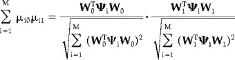
• 3All estimates of per‐voxel power or statistical change can be made sequentially and have no influence on other voxels in the source space [Van Veen et al., 1997]
• 4There is no tendency for sources to drift to the surface (as in typical minimum norm based approaches) [Grave de Peralta‐Menendez and Gonzales‐Andino, 1998]
• 5The solutions depend on data covariance and can therefore be used to image changes in spectral power that are not necessarily phase‐locked to a stimulus, such as ERD and ERS [Pfurtscheller and Lopes da Silva, 1999]
• 6A statistical difference calculation can be made at all points within a 3D volume giving SPMs of activity that, given anatomical information, can be transformed into standard space to produce group statistical maps [Singh et al., 2001, 2002].

The main limitations of using beamformer techniques are that:

• 1Any spatially separate yet covariant sources will be suppressed [Mosher et al., 1992; Mosher and Leahy 1998; Van Veen et al., 1997]. It has been shown, however, that temporal correlation must be relatively high (>0.7) before cancellation takes place [Van Veen et al., 1997]. These effects are further mitigated by using longer stretches of data that are presumably less likely to contain perfectly covariant activity over the whole time window.
• 2The spatial smoothness of the resulting SPMs will be inhomogeneous and anisotropic and will require statistical flattening before any corrections for multiple comparisons can be made. This is complicated by the fact that the beamformer weights are data dependent and therefore the spatial resolution at any region of the source space will depend on the particular dataset analysed.

In this work, this second limitation of beamformer‐based analysis is addressed. Our approach is to split the beamformer design and statistical imaging stages into distinct steps. We show how measures of spatial smoothness can be used to characterize the properties of the beamformer. We present a statistical framework, based on the functional magnetic resonance imaging (fMRI) and positron emission tomography (PET) literature [Andrade et al., 2001; Kiebel et al., 1999; Worsley et al., 1999], to statistically flatten the images and allow for correction of multiple comparisons.

We describe a modification of a standard minimum variance beamformer [Robinson and Vrba, 1999; Van Veen et al., 1997] in which the weight calculation and statistical test stages are treated separately. We point out how the weights, and hence the beamformer properties, are determined entirely by the data window over which the covariance is estimated (the covariance window).

We also derive analytical formulae that describe the underlying image smoothness, or full width half maximum (FWHM) of a Gaussian point spread function, in terms of the beamformer weights. Having calculated image smoothness, we then show how a choice of appropriate contrast windows can be used to calculate a beamformer‐based SPM.

The validity of our approach is demonstrated with simulation studies. We show the effect of source amplitude on the effective FWHM at each point in the resulting SPMs. Given these smoothness estimates, we show how statistical flattening [Worsley et al., 1999], based on the resel count for individual image voxels, can be used to correct for false positive rates across the inhomogeneously smooth SPMs.

MATERIALS AND METHODS

The data processing path for beamformer‐based analysis is outlined in Figure 1. MEG data is collected over a number of epochs, each containing a stimulus or task window and a rest period. Some time, or time‐frequency, range within each epoch is used to define a covariance window (T_cov). The choice of covariance window ultimately determines the spatial filter properties of the beamformer. For each possible source θ a weight vector W _θ, or spatial filter, is calculated. The output of this spatial filter, when applied to the MEG data, gives an estimate of the electrical activity, termed virtual electrode output, at θ. Defining a contrast window to consist of a pair of time (or time‐frequency) segments T_active and T_passive, a statistical parameter at θ can be computed from measures of spectral power change across all pairs of contrast windows. A volumetric SPM is computed from the iteration of the above procedure throughout the source space.

Figure 1.

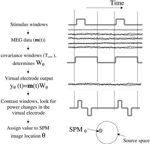
Schematic showing the partitioning of MEG data and the processing steps involved in making the SPM. The MEG data (m(t)) can be divided into epochs, each epoch containing a stimulus or task‐related time period defined by a stimulus window. A data segment of interest, or covariance window (T_cov), is used to calculate the MEG data covariance that in turn will determine the properties of the spatial filter (W _θ). At each source location θ, the spatial filter gives rise to an estimate of the electrical activity (or virtual electrode output y _θ(t)). A SPM value at θ is produced by statistical comparisons made on the virtual electrode output between the time‐frequency ranges specified by the contrast windows (in this case T_active and T_passive).

More formally, let m(t) be a column vector of N MEG channels at a single time instant t. Define a spatial filter centered on dipolar source element θ by the column vector of N coefficients W _θ. Where θ is made up of both dipole location and orientation parameters. In this study, for simplicity, we deal with the case in which all parameters of θ are known; in practice, either orientation is estimated [non‐linear beamformer: Vrba and Robinson, 2001] or calculations are made at orthogonal orientations and summed [linear beamformer: Van Veen et al., 1997] or alternatively, cortical surface information is made use of (work in progress).

The beamformer estimate of activity at element θ is given by:

(1)

For a minimum variance beamformer [Robinson and Vrba, 1999; Van Veen et al., 1997], weights are calculated so as to minimise the projected power at each source location subject to the constraint that the filter maintains a unity passband at this point.

The estimated power at source θ is given by:

(2)

where C is the N × N covariance matrix calculated over the covariance window (T_cov). It should be noted that projected power is only minimized over this window [Capon, 1969].

(3)

Define H _θ to be an N column vector containing the lead field of source θ (the lead field is defined as the signal produced in all sensors by a unit source at that location and orientation).

The linear constrained minimum variance beamformer can be expressed as:

(4)

That is, the weights are chosen so that the power at source θ is minimised subject to the constraint that the spatial filter maintains a unity passband at this point.

The solution to equation (4) is [Van Veen et al., 1997]

(5)

That is, the choice of covariance window completely determines the spatial filter, or weights W _θ, for any source θ. Using equations (2) and (5), the source power within the covariance window can be directly computed:

(6)

One problem with this measure is that noise at the sensors is aliased nonuniformly throughout the source space [Robinson and Vrba, 1999; Van Veen et al., 1997]. For a single sample test statistic therefore it is necessary to compensate for this effect by including a noise term in the denominator.

(7)

where X_θ is the neural activity index [Van Veen et al., 1997] or pseudo‐Z [Robinson and Vrba, 1999] at θ and Σ is the covariance matrix of channel noise.

For a two‐sample test statistic, however, this normalization stage becomes redundant. Rather than use the neural activity index as a metric of source strength, we use a statistical quantity describing the change in power at θ between contrast windows (in this case, T_active vs. T_passive). Although sensor noise will still be non‐uniformly distributed throughout the source space, in any two sample comparison it will be a constant (given that the sensor noise is stationary) affecting the magnitude of the two power measures at θ, but not the statistical difference between them. Let the estimated source power in any time‐frequency interval at source θ be given by

(8)

For each epoch i, divided into active and passive time portions of a contrast window, these power estimates can be expressed as:

(9)

(10)

where Y_θ ^act(i) is a measure of the power in the ith active time window over frequency band f_test. For example, the power in the 8–10 Hz band (f_test) over time 0–2 sec (T_active).

For a total of I_act and I_pass individual contrast windows, the SPM value for element θ can be obtained from the two‐sample t‐test (with degrees of freedom G = I_act + I_pass − 2) on the change in source power at θ. In this work we do not consider the case where contrast windows overlap, which would reduce the effective degrees of freedom. All power estimates are based on Hanning windowed data and therefore, even when time windows abut, the effect of the temporal correlations at the window edges due to filtering is negligible.

Note that the algorithm implemented by Robinson and Vrba [1999] and Vrba and Robinson [2001] differs from the above in two important respects.

First, Robinson and Vrba assume that the error variance in their pseudo‐Z statistic is due to the sensor noise alone (equation 7) and not variability in the neural signal.

Second, in the algorithms presented by Robinson and Vrba, there is no distinction between covariance and contrast windows. That is, when two time‐frequency windows are defined, the average covariance across both windows determines the beamformer properties and the power difference between the two windows, obtained from equation (6) directly, gives a measure of the statistical difference. In our analysis, there is a decoupling of beamformer design and statistical test stages such that the beamformer weights can be estimated based on broadband data whereas statistical tests can be carried out on narrow time‐frequency ranges within this broad time‐frequency window. In our experience, although narrow (time or frequency) contrast windows are often desirable, narrow covariance windows are not. The reason being that covariance estimates based on low degrees of freedom will tend to overestimate covariance between channels; in this case the beamformer will use these spurious correlations to suppress apparently (but not truly) covariant sources.

Computation of spatial smoothness

Estimates of SPM smoothness are necessary to calculate the number of independent image components or resels. In techniques such as fMRI and PET, image smoothness is generally most robustly computed from local correlations within images of the random elements or residuals [Kiebel et al., 1999] left over from the general linear model (GLM) fit. Correction for false positive error rates can then be based on the number of resels within the source space [Poline et al., 1995; Worsley et al., 1996, 1999].

As mentioned earlier, the characteristics of the MEG beamformer will depend on the data within the covariance window. The SPMs produced by any beamformer‐based algorithm, however, can be thought of as originating from some generic scanner with inhomogeneous spatial passband. For any beamformer based algorithm, if random data is substituted for real data in the contrast windows, random volumetric SPMs will result. These random SPMs will, however, have the same spatial smoothness as the true SPM produced from the real data (the spatial smoothness is governed by the weight vectors that are kept identical for the random and real data). Local spatial gradients in the resulting images then give smoothness estimates within the source space. To present a unified format to the functional imaging literature we shall refer to these projections of random data as ‘residuals’ although this is not strictly true. Note that this method relies on the assumption that source‐space smoothness measures are adequate to estimate the number of independent components within the SPMs (see Discussion ).

More formally, assume that the beamformer has already been designed for a particular covariance window in some real data set, giving weights W _θ for every source element θ.

To generate residuals we substitute white noise in place of the MEG data in the contrast windows.

Let η(t) be a time series of Gaussian white noise in N MEG channels.

The random time series n _θ(t) at virtual electrode θ is given as

(11)

Arbitrarily assigning two sections of η(t) to be T_active and T_passive, the residual (null signal) for any realisation i of η(t) at θ is given

(12)

Setting all residuals from M realisations of T_active and T_passive to have unit norm gives

(13)

where μ_iθ is the normalised residual at θ for noise realisation i.

Following Worsley et al. [1999], we divide the cubic lattice that forms the source space into a tetrahedrally connected mesh (five tetrahedra per voxel). For clarity at this point we introduce a parallel notation and define source element θ to be at location 0 and the connecting vertices of a single tetrahedral element to be at locations 1, 2 and 3. Then μ_i0, μ_i1, μ_i2, μ_i3 are the normalized residuals at element θ (or element 0) and its neighbouring elements (1–3) at realisation i. The image smoothness is estimated from the differences between the normalized residuals Δμ_θ containing M rows, where the ith row can be expressed as:

(14)

The resolution element or resel estimate at point θ, r(θ), is given by [Worsley et al., 1999]

(15)

Converting back into a cubic lattice simply involves summing the resels within each voxel (v), giving r(v). Assuming that the voxels are cubic of side length dx, then the filter FWHM at any voxel v is given by:

(16)

As mentioned above, equation (16) can be evaluated empirically using residuals projected from realisations of random data. A more elegant approach, however, is to use the fact that the correlations between residuals are intrinsically linked to the correlations between weights (see Appendix). Letting c_jk be the Pearson product moment correlation coefficient between weight vectors W _j and W _k

(17)

The elements of Δμ_θ ^TΔμ_θ can be expressed as

(18)

Where the elements of Δμ_θ ^TΔμ_θ are given by

(19)

For the diagonal elements, this simplifies to

(20)

SIMULATION SET‐UP

Smoothness estimates

In the first stage of the analysis we used simulated data to examine our smoothness metric. For all simulations we used the configuration of a 151 channel CTF Omega system [Vrba et al., 1999]. A source space was formed based on a subject's head outline as measured during an experimental recording session. The source space was divided into a regular 3D lattice (0.2 cm side length) of source elements (or potential current dipoles). The orientation of each element was set to be orthogonal to both the line joining it to the sphere centre and the vector defining the posterior–anterior direction. An active dipolar source was simulated at a depth of 3 cm from the scalp surface at 14 different source strengths (ranging from 0.1–200 nAm). The source was given a sinusoidal activation profile lasting for 100 msec and of period 20 msec; 100 epochs of MEG data were simulated with a per‐channel white noise level of 90 fT rms (10fT/√Hz, 81 Hz bandwidth). All forward problem and lead field calculations used the best fitting sphere to the subject's head outline as a volume conductor model. Beamformers were designed for each data set using covariance windows of 200 msec spanning 100 msec of activation and 100 msec of preceding white noise. The time‐frequency contrast windows used were the 100 msec of activation (T_active) and the 100 msec pre‐activation (T_passive) in the 40–60 Hz band (f_test). Estimates of smoothness were either estimated from 50 randomly generated sets of residual data (equations 11, 12) or calculated directly from the neighbouring weight vectors (equations (17), (18), (19), (20)).

False positive rate

We set out to investigate the statistical thresholds necessary to set corrected type‐1 error rates for the SPMs produced by the above simulations. We did this by using a pre‐existing set of beamformer coefficients and simulating a situation in which there was no statistical difference between contrast windows. Any SPM values that crossed a preset threshold would be due to chance alone. The beamformer designed for the data from the 0.2 nAm source in the above simulations was used; however in this simulation, the contrast windows spanned sections of MEG data that contained only Gaussian white noise (and no signal) (equations 11, 12). For each realisation (of 100 epochs of data) a single random volumetric SPM was produced (a two‐ sample t‐statistic with 198 df). For computational efficiency, each SPM was generated on a cubic lattice of side 1cm hence the necessity of choosing a source amplitude (0.2 nAm) known to give a minimum FWHM of greater than 2 cm (see results, Fig. 3). This null‐hypothesis scenario was repeated 3,000 times to produce estimates of the Type 1 error rate for specific choices of t‐statistic threshold. For each image, the error rate count was incremented (by one) if any voxel within the source space exceeded its preset threshold. Only voxels within the head volume were used in the analysis. We calculated false positive rates for both global and voxel‐wise thresholding.

Figure 3.

FWHM at the dipole location vs. source strength for a dipole simulated at approximately 3 cm depth for both analytical (solid) and empirical (dotted) smoothness estimates. As SNR increases the spatial filter becomes increasingly selective. The saturation (here at FWHM = 4 mm) is due to the spatial under‐sampling of the grid (2 mm spacing here). Note also that the analytical and empirical smoothness estimates are in good agreement.

Thresholds were set based on the expected value of the Euler characteristic of the 3D SPM [Worsley et al., 1996]. The expected number of excursion sets (or clusters) m to exceed threshold U is given by

(21)

where R_d are the d‐dimensional resel counts and ρ _d(U) is the d‐dimensional Euler Characteristic density function for a t‐statistic threshold U [Worsley et al., 1996].

The total resel count (or volume) was calculated analytically from the beamformer coefficients, by summing over all the voxels in the head volume. Resel counts for each dimension R_d were calculated given the assumption that this volume was also approximately spherical in resel space [Worsley et al., 1996].

From Friston et al. [1996a], the probability of obtaining at least one cluster of spatial extent r resels or more, exceeding a threshold U is given by

(22)

Where the above probability that the cluster contains at least r resels is given by

(23)

and

(24)

where the dimensionality of the SPM is set by D (=3), R is the total resel volume, Φ is the cumulative density function for the unit Gaussian distribution and Γ denotes the gamma function.

We used two different thresholding approaches: local and global. For local thresholding we treated each SAM voxel as a single cluster of volume r(v) resels. For a given false positive rate we then calculated the threshold level U(v) that one would expect a cluster of this size to exceed. For global thresholding, we looked at the effect of the assumption of uniform SPM smoothness on the false positive rate, and used the mean resel volume r _av to set the same threshold at all voxels, where

(25)

Where r _av is the mean resel volume, R is the total resel volume, and Nvoxels is the total number of voxels. The above measures were computed directly from the SPM matlab function spm_P.m (http://www.fil.ion.ucl.ac.uk/spm, 01/12/2001).

RESULTS

Smoothness estimates

The measure of spatial smoothness derived in the previous section gives an insight into the performance of the algorithm for a given covariance window. For a single simulated source we investigated the effect of SNR on both the spatial smoothness and the resulting SPM.

Figure 2A,C shows roughness (1/FWHM) in the coronal plane of voxels passing through the location of the simulated source at 3 cm depth for current densities of 2 and 10 nAm respectively. The roughness image peaks at the source location showing that voxels in this region have the smallest FHWM, that is, weight vectors relating to adjacent sources are changing the fastest. This is an intuitive property of a minimum variance beamformer, which strives to minimise its spatial passband to minimise estimated source power (equation 4). Comparing Figures 2A and C shows that as the source power increases the rougher the source space, or the more focal the eventual t‐SPM, becomes.

Figure 2.

Plots of spatial roughness (1/FWHM) of residual images (A,C) and subsequent SPM images (B,D) for source strengths 2 and 10 nAm respectively at a fixed dipole location (3 cm depth). The maps are in the coronal (x) plane with the z axis in the inferior‐superior direction passing through the dipole location and 1 cm anterior to the sphere centre. For (A,C), the maps are roughest, or least smooth, at the location of the simulated source. Note the change in smoothness across the images of approximately an order of magnitude. Also observable (A,C) are roughness peaks close to the sphere center, these peaks seem to arise due to numerical instability as the magnitudes of the lead field vectors approach 0. In this case, the minimum FWHMs are 8 mm and 5 mm for source of strengths of 2 and 10 nAm respectively. The SPMs were computed, based on a two‐sample t‐statistic, by using a contrast window in which T_passive and T_active contain data from 100 msec before and during the signal, respectively. The roughness maps depend solely on the choice of covariance window, whereas the t‐maps depend on the choice of contrast window as well.

In Figure 2B,D the SPMs for the optimal contrast windows (comparing the time window containing the signal with a pre‐stimulus baseline period) are shown. As predicted from the smoothness measures, the SPMs are more focal for the higher source strength. The critical difference between the SPMs and the smoothness measures is that the smoothness measures depend uniquely on the choice of covariance window whereas the SPMs depend on both the covariance window and the contrast windows chosen. That is, the smoothness measures describe the properties of the beamformer whereas the SPMs show the changes in estimated source power for a particular experimental hypothesis.

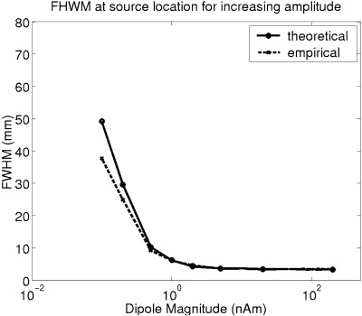
In Figure 3 the relationship between FWHM and source strength, hinted at in Figure 2, is examined in more detail. Both empirical (dotted) and analytical (solid line) estimates of FWHM at the simulated source location are plotted as functions of source strength. It is clear that the analytical estimates based on the correlations between weights (equations (17), (18), (19), (20)) and empirical results from generating pseudo‐residual images (equations 11, 12) are in good agreement. FWHM is clearly inversely related to source strength, however in this case it saturates at 4 mm. This saturation is due to spatial under‐sampling causing a degradation in the measure of resels as FWHM approaches twice the grid spacing (in this case 2 mm) [Friston et al., 1996a].

False positive rate

Using the beamformer designed for the 0.2 nAm source (see Materials and Methods ) we computed the type‐1 error rate in the SPMs for contrast windows consisting of Gaussian white noise for different thresholding strategies. Ideal performance, that is, where required and achieved error rates are identical, is shown as a dotted line in Figure 4. Global measures (dotted line), where the assumption is that the SPMs are uniformly smooth (equation 25), give rise to slightly inflated false positive rates (see discussion). Using local thresholding (solid line), where each voxel is assigned a different threshold level dependent on its extent in resel space, leads to a more accurate prediction of error rate. Figure 4B shows the distribution of per‐voxel threshold levels across the image as compared to the global threshold estimate for a corrected significance level of P < 0.05. The large spread of per‐voxel thresholds (due to variations in image smoothness) helps explain the differences observed in Figure 4A.

Figure 4.

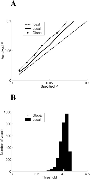
(A) The false‐positive error rate per SPM volumetric image for the beamformer weights designed for the 0. 2 nAm source at 3 cm depth. Ideal false positive rates, where the achieved rate should match the required rate are shown as a dotted line. The use of a global thresholding strategy (circles), where uniform smoothness is assumed, tends to produce over inflated error rates. The use of local thresholding (solid), where the threshold for each voxel is determined from its extent in resel space, is very close to ideal. (B) The distribution of per voxel thresholds (histogram) as compared to the global threshold (point) for corrected significance level P < 0.05. It is clear that there is a wide spread of per voxel thresholds, being lowest around the simulated source, where the images are least smooth (Fig. 2).

DISCUSSION

We have described a method for assessing the spatial smoothness of MEG beamformer based statistical parametric maps. Simple analytical expressions relating correlations between adjacent weight vectors to image smoothness have been derived and are in good agreement with our simulations (Fig. 3). The statistical images produced are least smooth (i.e., have lowest FWHM) around electrical sources and FWHM decreases with increasing source strength as has been previously reported [Gross et al., 2001; Van Veen et al., 1997; Vrba and Robinson, 2001]. The spatial smoothness measure enabled us to derive per voxel threshold levels that account for the inhomogenous smoothness of the images. The accuracy of these estimates depends however on adequate sampling of the source space (Fig. 3). We have shown that using these spatial smoothness measures it is possible to set accurate corrected false‐positive error rates for the SPMs (Fig. 4).

The method we propose differs slightly from that of other beamformer based algorithms such as SAM [Robinson and Vrba, 1999], the critical difference being that one can compute weights based on wide‐band data yet make statistical comparisons on narrow‐band data within this. SAM is a special case of this approach, where the same data is used to compute the weights and make the statistical comparison. The main advantage of our algorithm is that it enables a compromise between the signal suppression implicit in beamformers constructed from narrow‐band data (due to spurious correlations) and the decrease in beamformer spatial resolution when constructed from wide‐band data (due to lower SNR).

Although the Student t‐statistic is used throughout this work, it is a subject for further investigation as to whether it is the most appropriate test given the nature of the MEG data arising from ERD/ERS phenomena in the brain. Further work needs to address whether non‐parametric tests may be more appropriate. In future we anticipate the need to move to more versatile statistical analyses, such as the General Linear Model [Friston et al., 1995] to allow for the incorporation of other variables such as models of habituation [Friston et al., 1996b] or different time‐frequency ranges.

In this study we dealt exclusively with contrast windows that have no temporal overlap and have been considered to be independent. Due to the high temporal resolution of MEG, the time constant of the post‐synaptic potential (∼10 msec) and the fact that even abutting contrast windows are Hanning windowed before analysis, this assumption is reasonable. In selecting distinct analysis windows, however, we have sacrificed the temporal resolution of the statistical comparison for statistical power. Future work should allow for the comparison of overlapping contrast windows and incorporate adjustment of the degrees of freedom estimate to take this into account.

The smoothness estimates used here to calculate the degree of independence between the source space elements clearly rely on the assumption that only local correlations between voxels exist (as in smoothed fMRI and PET images). In MEG data, where each virtual electrode is formed from a linear mixture of the recording channels there is also the possibility of correlations between distant voxels. It is therefore doubtful that this result will generalize to any linear inverse solution (such as minimum norm). The minimum variance beamformer, however, is designed to minimise correlations between sources and this becomes most efficient as the sources become spatially separated [Van Veen et al., 1997]. The algorithm attempts to assign nominally orthogonal components of the signal space to different spatial locations; these orthogonal components can be thought of as the time‐courses within nominally independent (but oddly shaped) voxels. The results are still surprisingly accurate (Fig. 4A), especially given that for N channels there can be at maximum N independent virtual electrodes. Perhaps this last fact accounts for the slightly higher than specified false‐positive rate.

The SPMs are highly inhomogeneous in smoothness, with typical FWHMs varying over at least an order of magnitude (Fig. 2). In our error rate simulations we were forced to use a very low source power to keep the spatial sampling rate at a computationally manageable level (given that there were 3,000 simulations). Thus, although the results show similar error rates for local and global measures (Fig. 4), we predict that the global measures will continue to diverge from ideal as the images become less smooth. In practice, the computational burden of high spatial sampling could be relieved as it need not be regular; we anticipate a scheme whereby spatial sampling is increased locally until the estimated resel volume reaches a constant.

The statistical flattening described can be simply formulated in fewer dimensions [Worsley et al., 1999] and, in a similar manner to that being used in fMRI [Andrade et al., 2001], we anticipate its use with virtual electrode sites that are mapped directly to the cortical surface.

Most importantly, knowledge of both image smoothness and corrected significance levels is essential to make quantitative comparisons of statistical parametric maps across scanning modalities [Barnes et al., 2001; Taniguchi et al., 2000; Singh et al., 2001, 2002].

We show the relationship between the correlation between weights and the correlation between residuals. As an example we derive an expression for the sum of the squares of the differences between normalized residuals (the term a₁₁ in equation 18).

Equation (12), which gives the change in source power (or residual) at source element θ, can be re‐expressed in terms of the weights

(26)

Where N ₁ and N ₂ are the expected covariance matrices of channel noise over time periods T _active and T _passive respectively.

(27)

and m is a constant normalizing for the number of samples in T _active and T _passive. The residual can be expressed as

(28)

or, defining

(29)

gives

(30)

The normalized residual at realization i is given by

(31)

Examining term a₁₁ in equation (18)

(32)

As the sum of the square of the normalized residuals is defined to be unity (equation 13)

(33)

Where the summation term is simply the correlation between the normalized residuals (that is the same as the correlation between residuals).

Evaluating the summation

(34)

As Ψ_i is diagonal, this simplifies to

(35)

and, as the covariance matrix of weight vectors is symmetric

(36)

the correlation between residuals is given by

(37)

that is equivalent to the square of the correlation between the weights (equation 17)

(38)

Hence, (see also equation 20):

(39)

REFERENCES

- Andrade A, Kherif F, Mangin JF, Worsley KJ, Paradis AL, Simon O, Dehaene S, Le Bihan D, Poline JB (2001): Detection of fMRI activation using cortical surface mapping. Hum Brain Mapp 12: 79–93. [DOI] [PMC free article] [PubMed] [Google Scholar]
- Barnes GR, Francis S, Hillebrand A, He J, Furlong PL, Bowtell RW, Singh KD, Holliday IE, Morris PG (2001): The spatial relationship between event‐related changes in cortical synchrony and the haemodynamic response. Neuroimage 13: S71. [Google Scholar]
- Capon J (1969): High‐resolution frequency‐wavenumber spectrum analysis. Proc IEEE 57: 1408–1419. [Google Scholar]
- Cheyne D, Barnes GR, Holliday IE, Furlong PL (2000): Localization of brain activity associated with non‐time‐locked tactile stimulation using synthetic aperture magnetometry (SAM) In: Neonen J, Ilmoniemi T, Katila T, editors. 12th International Conference on Biomagnetism. Espoo, Finland: Helsinki Univ. of Technology; p 255–258. [Google Scholar]
- Friston KJ, Holmes A, Poline JB, Price CJ, Frith CD (1996a): Detecting activations in PET and fMRI: levels of inference and power. Neuroimage 4: 223–235. [DOI] [PubMed] [Google Scholar]
- Friston KJ, Holmes AP, Worsley KJ, Poline J‐B, Frith CD, Frackowiak RS (1995): Statistical parametric maps in functional imaging: a general linear approach. Hum Brain Mapp 2: 189–210. [Google Scholar]
- Friston KJ, Stephan KM, Heather JD, Frith CD, Ioannides AA, Liu LC, Rugg MD, Vieth J, Keber H, Hunter K, Frackowiak RS (1996b): A multivariate analysis of evoked responses in EEG and MEG data. Neuroimage 3: 167–174 [DOI] [PubMed] [Google Scholar]
- Grave de Peralta‐Menendez R, Gonzales‐Andino SL (1998): A critical analysis of linear inverse solutions to the neuroelectromagnetic inverse problem. IEEE Trans Biomed Eng 45: 440–448. [DOI] [PubMed] [Google Scholar]
- Gross J, Kujala J, Hamalainen M, Timmermann L, Schnitzler A, Salmelin R (2001): Dynamic imaging of coherent sources: studying neural interactions in the human brain. Proc Natl Acad Sci U S A 98: 694–699. [DOI] [PMC free article] [PubMed] [Google Scholar]
- Hashimoto I, Kimura T, Iguchi Y, Takino R, Sekihara K (2001): Dynamic activation of distinct cytoarchitectonic areas of the human SI cortex after median nerve stimulation. Neuroreport 12: 1891–1897. [DOI] [PubMed] [Google Scholar]
- Huang M, Aine CJ, Supek S, Best E, Ranken D, Flynn ER (1998): Multi‐start downhill simplex method for spatio‐temporal source localization in magnetoencephalography. Electroencephalogr Clin Neurophysiol 108: 32–44. [DOI] [PubMed] [Google Scholar]
- Kiebel SJ, Poline JB, Friston KJ, Holmes AP, Worsley KJ (1999): Robust smoothness estimation in statistical parametric maps using standardized residuals from the general linear model. Neuroimage 10: 756–766. [DOI] [PubMed] [Google Scholar]
- Mosher JC, Leahy RM (1998): Recursive MUSIC: a framework for EEG and MEG source localization. IEEE Trans Biomed Eng 45: 1342–1354. [DOI] [PubMed] [Google Scholar]
- Mosher JC, Lewis PS, Leahy RM (1992): Multiple Dipole modeling and localization from spatio‐temporal MEG data. IEEE Trans Biomed Eng 39: 541–557. [DOI] [PubMed] [Google Scholar]
- Pfurtscheller G, Lopes da Silva FH (1999): Event‐related EEG/MEG synchronization and desynchronization: basic principles. Clin Neurophysiol 110: 1842–1857. [DOI] [PubMed] [Google Scholar]
- Pfurtscheller G, Stancak A Jr, Neuper C (1996): Event‐related synchronization (ERS) in the alpha band—an electrophysiological correlate of cortical idling: a review. Int J Psychophysiol 24: 39–46. [DOI] [PubMed] [Google Scholar]
- Poline JB, Worsley KJ, Holmes AP, Frackowiak RS, Friston KJ (1995): Estimating smoothness in statistical parametric maps: variability of p values. J Comput Assist Tomogr 19: 788–796. [DOI] [PubMed] [Google Scholar]
- Robinson SE, Rose DF (1992): Current source image estimation by spatially filtered MEG In: Hoke M, Erné SN, Okada YC, Romani GL, editors. Biomagnetism: clinical aspects. Amsterdam: Elsevier Science Publishers; p 761–765. [Google Scholar]
- Robinson SE, Vrba J (1999): Functional neuroimaging by synthetic aperture magnetometry (SAM) In: Recent advances in biomagnetism. Sendai: Tohoku Univ. Press; p 302–305. [Google Scholar]
- Sekihara K, Nagarajan S, Poeppel D, Miyashita Y (1999): Time‐frequency MEG‐MUSIC algorithm. IEEE Trans Med Imaging 18: 92–97. [DOI] [PubMed] [Google Scholar]
- Singh KD, Barnes GR, Hillebrand A (2001): An MEG/fMRI multi‐modality study of biological motion processing: group analysis of “boxcar” MEG data using Synthetic Aperture Magnetometry. Neuroimage 13: S247. [Google Scholar]
- Singh KD, Barnes GR, Hillebrand A, Forde EME, Williams AL (2002): Task‐related changes in cortical synchronisation are spatially coincident with the haemodynamic response. Neuroimage 16: 103–114. [DOI] [PubMed] [Google Scholar]
- Supek S, Aine CJ (1993): Simulation studies of multiple dipole neuromagnetic source localization: model order and limits of source resolution. IEEE Trans Biomed Eng 40: 529–540. [DOI] [PubMed] [Google Scholar]
- Taniguchi M, Kato A, Fujita N, Hirata M, Tanaka H, Kihara T, Ninomiya H, Hirabuki N, Nakamura H, Robinson SE, Cheyne D, Yoshimine T (2000): Movement‐related desynchronization of the cerebral cortex studied with spatially filtered magnetoencephalography. Neuroimage 12: 298–306. [DOI] [PubMed] [Google Scholar]
- Van Veen BD, van Drongelen W, Yuchtman M, Suzuki A (1997): Localization of brain electrical activity via linearly constrained minimum variance spatial filtering. IEEE Trans Biomed Eng 44: 867–880. [DOI] [PubMed] [Google Scholar]
- Vrba j, Anderson G, Betts K, Burbank MB, Cheung T, Cheyne D, Fife AA, Govorkov S, Habib F, Haid G, Haid V, Hoang T, Hunter C, Kubik PR, Lee S, McCubbin J, McKay J, McKenzie D, Nonis D, Paz J, Reichl E, Ressl D, Robinson SE, Schroyen C, Sekatchev I, Spear P, Taylor B, Tillotson M, Sutherling W (1999): 151‐Channel whole‐cortex MEG system for seated or supine positions In: Recent advances in biomagnetism. 11th International Conference on Biomagnetism. Sendai: Tohoku Univ. Press. [Google Scholar]
- Vrba J, Robinson SE (2001): Differences between synthetic aperture magnetometry (SAM) and linear beamformers In: Neonen J, Ilmoniemi T, Katila T, editors. 12th International Conference on Biomagnetism. Espoo, Finland: Helsinki Univ. of Technology; p 681–684. [Google Scholar]
- Worsley KJ, Marrett S, Neelin P, Vandal AC, Friston KJ, Evans AC (1996): A unified statistical approach for determining significant signals in images of cerebral activation. Hum Brain Mapp 4: 58–73. [DOI] [PubMed] [Google Scholar]
- Worsley KJ, Andermann M, Koulis T, MacDonald D, Evans AC (1999): Detecting changes in nonisotropic images. Hum Brain Mapp 8: 98–101. [DOI] [PMC free article] [PubMed] [Google Scholar]