

Abstract
We have applied the eigenspace‐based beamformer to reconstruct spatio‐temporal activities of neural sources from MEG data. The weight vector of the eigenspace‐based beamformer is obtained by projecting the weight vector of the minimum‐variance beamformer onto the signal subspace of a measurement covariance matrix. This projection removes the residual noise‐subspace component that considerably degrades the signal‐to‐noise ratio (SNR) of the beamformer output when errors in estimating the sensor lead field exist. Therefore, the eigenspace‐based beamformer produces a SNR considerably higher than that of the minimum‐variance beamformer in practical situations. The effectiveness of the eigenspace‐based beamformer was validated in our numerical experiments and experiments using auditory responses. We further extended the eigenspace‐based beamformer so that it incorporates the information regarding the noise covariance matrix. Such a prewhitened eigenspace beamformer was experimentally demonstrated to be useful when large background activity exists. Hum. Brain Mapping 15:199–215, 2002. © 2002 Wiley‐Liss, Inc.
Keywords: magnetoencephalography, biomagnetism, MEG inverse problems, beamformer, functional neuroimaging, neuromagnetic signal processing
INTRODUCTION
Among the various kinds of functional neuroimaging methodologies, magnetoencephalography (MEG) has the the major advantage that it can provide fine time resolution of the millisecond order [Hämäläinen et al., 1993]. Neuromagnetic imaging can thus be used to visualize neural activities with such a fine time resolution and to provide functional information about brain dynamics [Roberts et al., 1998]. Toward this goal, a number of algorithms for reconstructing spatio‐temporal source activities have been investigated.
In our study, we explore the possibility of applying a class of techniques referred to as the adaptive beamformer to this spatio‐temporal reconstruction of the neural‐source activities. The adaptive beamformer provides a versatile form of spatial filtering, and it has been originally developed in the fields of array signal processing, including radar, sonar, and seismic exploration [van Veen and Buckley, 1988]. One well‐known technique of this kind, the minimum‐variance beamformer, has already been successfully applied to solve the MEG/EEG source‐localization problem [Gross and Ioannides, 1999; Robinson and Vrba, 1999; Spencer et al., 1992; van Veen et al., 1997]. We found, however, that the minimum‐variance beamformer generally is very sensitive to errors in the forward modeling or errors in estimating the data covariance matrix when it is applied to the reconstruction of source activities at each instant in time. Because such errors are almost inevitable in neuromagnetic measurements, the minimum‐variance beamformer generally provides noisy spatio‐temporal reconstruction results, as is demonstrated later in this study.
One technique has been developed to overcome the poor performance of the minimum‐variance‐based technique caused by the forward modeling errors [Cox et al., 1987] and covariance‐matrix estimation errors [Carlson, 1988]. The technique, referred to as the diagonal loading, uses the regularized inverse of the measurement covariance matrix, instead of its direct matrix inverse, when calculating the weight vector. Although this technique has been applied to the MEG source localization problem [Gross and Ioannides, 1999; Robinson and Vrba, 1999], it has been known that the regularization leads to a trade‐off between the spatial resolution and the SNR of the beamformer output. The results from our experiments demonstrate this trade‐off relationship.
We propose to apply the eigenspace‐based beamformer [Feldman and Griffiths, 1991; van Veen, 1988] to reconstructing spatio‐temporal activities of neural sources. The weight vector of the eigenspace‐based beamformer is obtained by projecting the weight vector of the minimum‐variance beamformer onto the signal subspace of the measurement covariance matrix. This projection removes a residual noise‐subspace component that considerably degrades the signal‐to‐noise ratio (SNR) of the beamformer output when the above‐mentioned errors exist. Therefore, the eigenspace‐based beamformer produces a SNR significantly higher than that from the minimum‐variance beamformer; thus, it is a suitable method for spatio‐temporal reconstruction of the neural source activities.
After a brief introduction to the minimum‐variance beamformer, we describe the principle of the eigenspace‐based beamformer. We also present a theoretical comparison between these beamformer techniques and numerical experiments that validate our arguments. We also describe the application of the beamformer techniques to auditory‐evoked responses. The results demonstrate that the eigenspace‐based beamformer techniques are highly effective for the spatio‐temporal reconstruction of source activities.
MATERIALS AND METHODS
Definitions and Fundamental Relationships
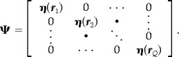
Let us define the magnetic field measured by the mth detector coil at time t as b m(t), and a column vector b(t) = [b 1(t), b 2(t),…, b M(t)]T as a set of measured data where M is the total number of detector coils and the superscript T indicates the matrix transpose. A spatial location is represented by a 3D vector r:r = (x,y,z). A total of Q current sources are assumed to generate the neuromagnetic field, and the locations of these sources are denoted as r 1, r 2,…, r Q. The moment magnitude of the qth source at time t is denoted as s(r q, t), and the source magnitude vector is defined as s(t) = [s(r 1, t), s(r 2, t)…, s(r Q, t)]T. The orientation of the qth source is defined as a 3D column vector η(r q, t) = [ηx (r q, t), ηy (r q, t), ηz (r q, t)]T whose ζ component (where ζ equals x, y, or z in this study) is equal to the cosine of the angle between the direction of the source moment and the ζ direction. We assume that the orientation of each source is time independent. Omitting the time notation t, we define a 3Q × Q matrix that expresses the orientations of all Q sources as Ψ such that
 |
Let us define l ( r) as the mth sensor output induced by the unit‐magnitude source located at r and directed in the ζ direction. The column vector l ζ(r) is defined as l ζ(r) = [l (r), l (r),…,l (r)]T. We define the lead field matrix, which represents the sensitivity of the whole sensor array at r, as L(r) = [l x(r), l y(r), l z(r)]. We define, for later use, the lead‐field vector in the source‐moment direction as l(r); it is obtained by using l(r) = L(r)η(r). The composite lead field matrix for the entire set of Q sources is defined as
| (1) |
The relationship between b(t) and s(t) is then expressed as
| (2) |
where n(t) is the additive noise.
Let us define the measurement covariance matrix as R b; i.e., R b = 〈b(t)b T(t)〉, where 〈 · 〉 indicates the ensemble average (this ensemble average is usually replaced with the time average over a certain time window). Let us also define the covariance matrix of the source‐moment activity as R s; i.e., R s = 〈s(t)s T(t)〉. Then, using equation (2), we get the relationship between the measurement covariance matrix and the source‐activity covariance matrix such that
| (3) |
where the noise in the measured data is assumed to be the white Gaussian noise with the variance of σ2 and I is the unit matrix.
Let us define the jth eigenvalue and eigenvector of R b as λj and e j, respectively. Unless some source activities are perfectly correlated with each other, the rank of R s is equal to the number of sources Q. Therefore, according to equation (3), R b has Q eigenvalues greater than σ2 and M–Q eigenvalues that are equal to σ2. Let us define the matrices E S and E N as E S = [e 1,…,e Q] and E N = [e Q + 1, …, e M]. The column span of E S is the maximum‐likelihood estimate of the signal subspace of R b and the span of E N is that of the noise subspace [Scharf, 1991]. Using equation (3), it can be shown that, at source locations, the lead field matrix with the correct source orientation is orthogonal to the noise subspace of the measurement covariance matrix [Schmidt, 1981], i.e.,
| (4) |
Minimum‐Variance Beamformer
To estimate the source moment, we have focused on using the class of techniques referred to as the spatial filter. The spatial filter techniques use the following simple linear operation for estimating the source moment,
| (5) |
where ŝ(r,t) is the estimated magnitude of the source‐moment at r and time t. In this equation, w(r) is a column vector characterizing the filter weight. Note that because this weight vector is calculated for any spatial location r, the source‐moment distribution can be reconstructed by scanning the output of the spatial filter over a region of interest in a perfectly post‐processing manner. One well‐known spatial filter of this kind is the minimum‐variance distortion‐less beamformer originally developed for seismic‐array signal processing [Capon, 1969]. In this technique, the filter weight vector w m(r) is obtained by minimizing w (r)R b w m(r) under the constraint of l T(r)w m(r) = 1. The explicit form of the weight vector for the minimum‐variance beamformer is known to be
| (6) |
This minimum variance beamformer has been one of the most popular spatial‐filter techniques in various signal‐processing fields. It has also been applied to neuromagnetic source localization [Robinson and Vrba, 1999; Spencer et al., 1992; van Drongelen et al., 1996; van Veen et al., 1997].
Eigenspace‐Based Beamformer
The eigenspace‐based beamformer [Feldman and Griffiths, 1991; van Veen, 1988; Yu and Yeh, 1995] provides an output SNR much higher than that of the minimum‐variance beamformer in practical situations. Let us decompose the measurement covariance matrix R b into its signal and noise subspace components; i.e.,
| (7) |
Here, we define the matrices ΛS and ΛN as
| (8) |
where diag[…] indicates a diagonal matrix whose diagonal elements are equal to the entries in the parenthesis. Using equations (6) and (7), and defining μ = 1/[l T(r)R b −1 l(r)], we express the weight vector for the minimum‐variance beamformer as
| (9) |
where
In equation (9), the second term on the right side, μΓ Nl(r), should ideally be equal to zero because the lead‐field vector l(r) is orthogonal to E N at the source locations as indicated by equation (4). Various factors, however, prevent this term from being zero, and a non‐zero μΓ Nl(r) seriously degrades SNR as explained in the next section. Therefore, the eigenspace‐based beamformer uses only the first term of equation (9) to calculate its filter weight vector w e(r); i.e.,
| (10) |
Note that w e(r) is equal to the projection of w m(r) onto the signal subspace of R b. The following relationship holds [Feldman and Griffiths, 1991]:
| (11) |
Comparison Between Minimum‐Variance and Eigenspace Beamformers
Although the minimum‐variance beamformer ideally has exactly the same SNR as that of the eigenspace‐based beamformer, the SNR of the eigenspace beamformer is significantly higher in practical applications, as demonstrated in the following sections. The reason of this high SNR can be understood as follows.
Let us assume that a signal source with a moment magnitude equal to s(t) exists at r. Then, the estimate of s(t), ŝ(t), is derived by ŝ(t) = w Tb(t) = w Tl(r)s(t) and the average power of ŝ(t), P̂ s, is expressed as
| (12) |
where P s is the average power of s(t) defined by P s = 〈s(t)2〉. Similarly, the average noise power contained in the estimated results, P̂n is given by
| (13) |
where we again assume that 〈n(t)n T(t)〉 = σ2 I. Thus, the output SNR of the minimum‐variance beamformer, SNR(MV), is expressed as [Chang and Yeh, 1992, 1993],
| (14) |
The SNR for the eigenspace‐based beamformer, SNR(ES), is obtained as
| (15) |
The only difference between equations, namely (14) and (15) is the existence of the second term l T(r)Γ l(r) in the denominator of the right‐hand side of equation (14). It is readily apparent that SNR(MV) and SNR(ES) are equal if we can use an accurate noise subspace estimate and an accurate lead‐field vector, because the term l T(r)Γ l(r) is exactly equal to zero in this case. It is, however, generally difficult to attain the relationship, l T(r)Γ l(r) = 0. One obvious reason for this difficulty is that when calculating Γ in practice, instead of using R b, the sample covariance matrix R̂ b must be used; R̂ b is calculated from R̂ b = Σ b(t k)b T(t k) where K is the number of time points. Use of the sample covariance matrix inevitably makes l T(r)Γ l(r) have a non‐zero value and causes SNR of the minimum‐variance beamformer to degrade [Richmond, 1998].
Another factor that is specific to MEG and causes l T(r)Γ l(r) to have a non‐zero value is that it is almost impossible to use a perfectly accurate lead‐field vector. This is because a conductivity distribution in the brain usually be approximated by using some kind of conductor model, such as the spherically homogeneous conductor model [Sarvas, 1987], to calculate the lead field matrix. Although this error may be reduced to a certain extent by using a realistic head model, the error cannot be perfectly avoided. Let us define the overall error in estimating l(r) as ϵ. Assuming that ∥l(r)∥2≫∥ε∥2, we can get
| (16) |
Note that, in the denominator of the right‐hand side of this equation, the norm of the matrix εTΓε has an order of magnitude proportional to ∥ε∥2/λ2, where λN represents one of the noise‐level eigenvalues of R b. The eigenvalue λN is usually significantly smaller than the signal‐level eigenvalues. Therefore, equation (16) indicates that even when the error ∥ε∥ is very small, the term εTΓε may not be negligibly small compared to the first term in the denominator.
Extension to Prewhitened Eigenspace Beamformer
Real‐life MEG data often contain interference arising from background brain activities [Sekihara et al., 1997]. Such interference does not affect the final reconstruction results if the sources of interference are spatially well separated from the signal source of interest. The influence, however, may not be negligible if the interference source is located close to the signal source (within the range of the spatial resolution). Such interference is known to cause spatially non‐white noise in neuromagnetic measurements, and if the information regarding the noise covariance matrix is obtained, the effect of such interferences can be significantly reduced by using the prewhitened eigenspace beamformer technique described below.
When the noise is nonwhite, equation (3) becomes
| (17) |
where R n is the noise covariance matrix obtained from R n = 〈n(t)n T(t)〉. Let us denote ẽ j as an eigenvector obtained by solving the generalized eigenvalue problem,
| (18) |
In this case, it is easy to show that the following orthogonality relationship holds,
| (19) |
where Ẽ N = [ẽ Q′ + 1,…,ẽ M] and Q′ is the number of sources. Thus, the signal subspace projector can be formed by using Ẽ S Ẽ , where Q̃ S = [ẽ 1,…,ẽ′ Q] and the weight vector for the prewhitened eigenspace beamformer, w̃ e(r), is obtained from
| (20) |
The effectiveness of the beamformer based on this equation in removing background interferences is demonstrated in the following sections.
NUMERICAL EXPERIMENTS
Data Generation
We conducted a series of numerical experiments to test the effectiveness of the eigenspace‐based beamformer techniques. The coil alignment of the 37‐channel Magnes™ biomagnetic measurement system (Biomagnetic Technologies Inc., San Diego) was used in these experiments. The coordinate origin was defined as the center of the detector coil located at the center of the coil alignment. Three signal sources were assumed to exist on a plane defined as x = 1.0 cm; their locations were (1, −1, −6), (1, 1, −6), and (1, 1.6, −7.2) cm. The source and detector configuration is shown schematically in Figure 1. The spherically homogeneous conductor model with the origin set at (1, 0, −11) (cm) was used. The magnetic field was generated at 1‐msec intervals from −300 to 400 msec. The time courses of the three source activities assumed in our numerical experiments are shown in Figure 2. The first and second sources were the sources of interest, and the third source simulated background interference. Gaussian noise was added to the generated magnetic field so that the SNR was set at 8 and the SNR was defined by the ratio of the Frobenius norm of the signal‐magnetic‐field data matrix to that of the noise matrix. The generated 37‐channel magnetic‐field recordings are also shown in Figure 2.
Figure 1.
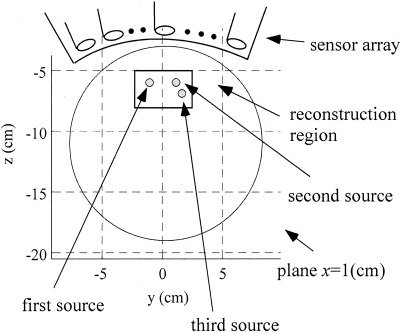
The source and detector configuration used in the numerical experiments. The circle shows the cross section of the sphere used for the forward calculation. The square shows the reconstruction region used for our numerical experiments.
Figure 2.
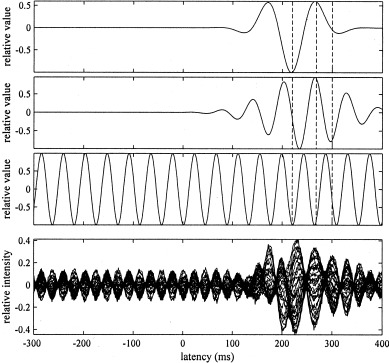
The moment time courses of the three sources assumed in the numerical experiments. Time courses from the first to the third sources are shown from the top to the third row, respectively. Each waveform is normalized by its maximum value and the three vertical broken lines show the three time points 220, 268, and 300 msec. The simulated 37‐channel magnetic field recordings are shown in the bottom row.
Spatio‐Temporal Reconstruction Experiments
The reconstruction region was set as an area defined by −2 ≤ y ≤ 2 and −8 ≤ z ≤ −5 (cm) (as indicated by the square in Fig. 1), and the interval of the reconstruction grid was 1 mm in both directions. In our experiments, when applying beamformer techniques, we first used the method described in the Appendix for estimating the optimum source orientation ηˆ opt and we then estimated the lead field vector l(r) = L(r)ηˆ opt at each scanning grid point. To display the results of the spatio‐temporal reconstruction, three time instants at 220, 268, and 300 msec (marked by three vertical broken lines in Fig. 2) were selected. The amplitude of the second source was zero at 220 msec, all the sources had non‐zero amplitudes at 268 msec, and only the second source had a non‐zero amplitude at 300 msec (Fig. 2). The measurement covariance matrix was calculated by using a time window between 0–400 msec. The power, averaged over this time window, of the second source is 1.5 times stronger than that of the first source.
Results From Minimum‐Variance Beamformer
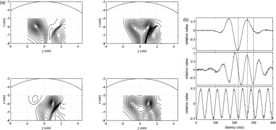
We first applied the minimum‐variance beamformer to the generated data set in Figure 2. The results of the spatio‐temporal reconstruction are shown in Figure 3a. Contour maps in the upper‐left, upper‐right and lower‐left positions indicate the distributions of the source‐moment power ŝ(r, t)2 at the three time instants of 220, 268, and 300 msec, respectively. The lower‐right contour map shows the time‐averaged reconstruction, obtained by averaging ŝ(r, t)2 over the time window from 0–400 msec. The estimated time courses at the pixels nearest to the three source locations are shown in Figure 3b. These results show that the spatio‐temporal reconstruction obtained by using the minimum variance beamformer was fairly noisy; that is, the estimated time courses contained a considerable amount of noise, and the three snapshots of the source activity contained the influence of this noisy reconstruction. The time‐averaged results, however, did not contain this influence and clearly detected the three sources.
Figure 3.
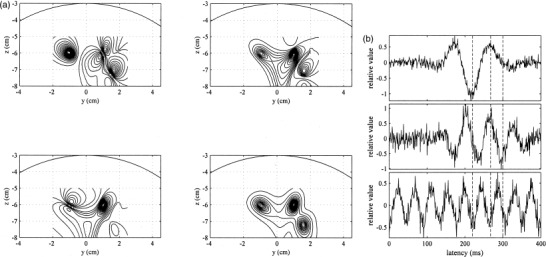
The results obtained using the minimum‐variance beamformer. (a) Snapshots of source activities at 220 msec (upper left), 268 msec (upper right), and 300 msec (lower left). The time‐averaged reconstruction is shown in the lower‐right position. The reconstructed region is indicated by the square in Figure 1. (b) Estimated time courses of the first source (top), the second source (middle), and the third source (bottom). The three vertical broken lines show the three time points 220, 268, and 300 msec.
Results From Minimum‐Variance Beamformer With Regularized Inverse
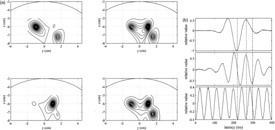
We next tested the minimum‐variance weight vector together with the use of the regularized inverse (R b + γI)−1. The regularization parameter was set at 0.003λ1 1 where λ1 is the largest eigenvalue of R b. The results of the reconstruction are shown in Figure 4a,b. The time course estimation in Figure 4b shows that the SNR of the beamformer output was greatly improved, but the contour maps in Figure 4a indicate that a considerable amount of blur was introduced. Our results here confirm the trade‐off relationship between the spatial resolution and the output SNR.
Figure 4.
The results obtained using the minimum‐variance beamformer with the regularized inverse. (a) Snapshots of source activities at 220 msec (upper left), 268 msec (upper right), and 300 msec (lower left). The time‐averaged reconstruction is shown in the lower‐right position. (b) Estimated time courses of the first source (top), the second source (middle), and the third source (bottom). The three vertical broken lines show the three time points 220, 268, and 300 msec.
Results From Eigenspace‐Based Beamformer
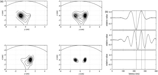
We applied the eigenspace‐based beamformer given by equation (10) to the same computer‐generated data set. The reconstructed source distributions are shown in Figure 5a, and the estimated time courses are shown in Figure 5b. These figures show that this beamformer technique considerably improved the output SNR with almost no sacrifice of spatial resolution.
Figure 5.
The results obtained using the eigenspace‐based beamformer. (a) Snapshots of source activities at 220 msec (upper left), 268 msec (upper right), and 300 msec (lower left). The time‐averaged reconstruction is shown in the lower‐right position. (b) Estimated time courses of the first source (top), the second source (middle), and the third source (bottom). The three vertical broken lines show the three time points 220, 268, and 300 msec.
Results From Prewhitened Eigenspace Beamformer
We tested the effectiveness of the prewhitened eigenspace beamformer proposed earlier in reducing the background interference; namely the influence from a third source. First, we estimated the noise covariance matrix using the prestimulus time window from −300–0 msec. We then applied the prewhitened eigenspace beamformer (equation (20)) with this estimated noise covariance matrix to reconstruct the source‐moment distribution (Fig. 6a). The estimated time courses are shown in Figure 6b. These results show that the influence of the third source was nearly completely removed. Also, the results in Figure 6b show that the time courses of the first and the second sources were not affected by the prewhitening procedure.
Figure 6.
The results obtained using the prewhitened eigenspace‐based beamformer. (a) Snapshots of source activities at 220 msec (upper left), 268 msec (upper right), and 300 msec (lower left). The time‐averaged reconstruction is shown in the lower‐right position. (b) Estimated time courses of the first source (top), the second source (middle), and the third source (bottom). The three vertical broken lines show the three time points 220, 268, and 300 msec.
APPLICATION TO AUDITORY‐EVOKED RESPONSES
Data acquisition Condition
To further demonstrate the superiority of the eigenspace‐based beamformer over the minimum‐variance beamformer, we applied these beamformer techniques to auditory‐evoked responses. Auditory‐evoked fields were measured by using the 37‐channel Magnes™ magnetometer installed at the Biomagnetic Imaging Laboratory, University of California, San Francisco. Healthy male volunteers participated in the MEG measurements. Their written informed consents were obtained and the MEG measurements were approved by the Committee on Human Research, University of California, San Francisco. All measurements were done in a magnetically‐shielded room. Auditory stimuli were presented to a subject's right ear. The sensor array was placed above a subject's left hemisphere with the position adjusted to optimally record the N1m auditory‐evoked field. The inter‐stimulus interval randomly varied between 1.75 sec and 2.25 sec, and the average interval was 2 sec. The sampling frequency was set at 1 kHz. An on‐line filter with a bandwidth from 1–400 Hz was used, and no post‐processing digital filter was applied. To express the results of reconstructing source activities in this section, we used the head coordinates illustrated in Figure 7.
Figure 7.
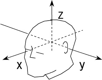
The x, y, and z coordinates used to express the reconstruction results in the application to auditory‐evoked responses. The midpoint between the left and right pre‐auricular points is defined as the coordinate origin. The axis directed away from the origin toward the left pre‐auricular point is defined as the +y axis and that from the origin to the nasion is the +x axis. The +z axis is defined as the axis perpendicular to both these axes and is directed from the origin to the vertex.
Results From Minimum‐Variance and Eigenspace Beamformer
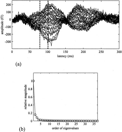
The auditory stimulus was a 1,000‐Hz pure tone, and we measured 256 epochs. The auditory‐evoked response averaged across these epochs is shown between 0–300 msec in Figure 8a. We applied the eigenspace‐based beamformer to reconstruct the spatio‐temporal source activities from this auditory data set. The time window ranging from 0–300 msec was used for calculating the covariance matrix R b. The eigenvalue spectrum of R b is shown in Figure 8b. The dimension of the signal subspace was set at 1 because the eigenvalue spectrum contained one distinctly large eigenvalue. Three time instants, 87, 90, 101 msec, were selected near the peak vertex of N100m. These instants are shown by three vertical broken lines in Figure 8a. The reconstructed source‐magnitude maps at these three latencies are shown in Figure 9a. These three snapshots of the source activities contain a single, sharply‐localized activity in the left temporal‐lobe, probably near the primary auditory cortex area. The time course in the maximum point in these contour maps is shown in Figure 9b. The time course has a clear negative peak near the latency of 50 msec and a large positive peak near the latency of 100 msec.
Figure 8.
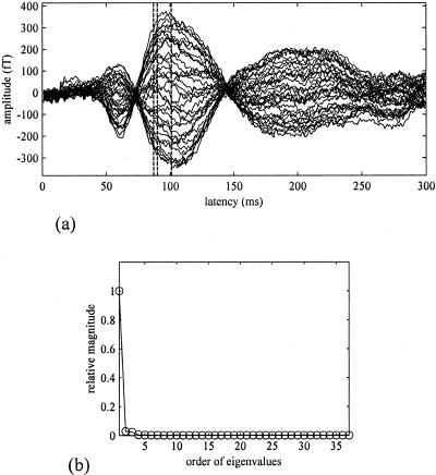
(a) Thirty‐seven channel recordings of auditory evoked magnetic field measured using a 1‐kHz pure tone. A total of 256 epochs were averaged. Three vertical broken lines indicate time instants at 87, 90, 101 msec, at which the snapshots of the source activity are shown in Figures 9a, 10a, and 11a. (b) Eigenvalue spectrum of R b obtained from the time window between 0 and 300 msec of the data set shown in (a).
Figure 9.
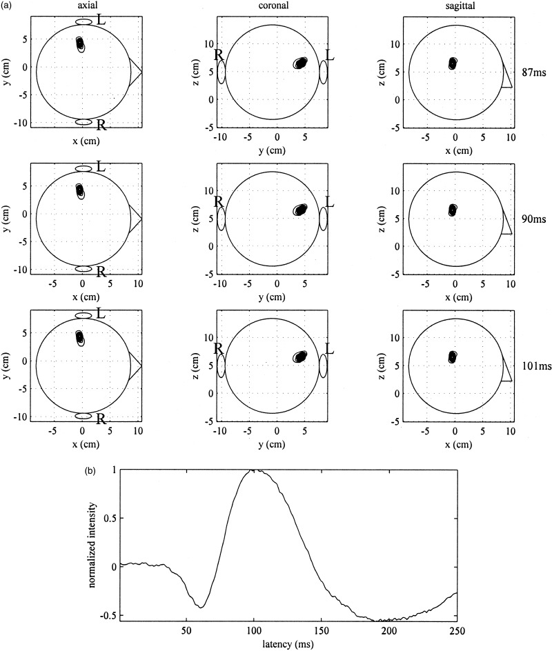
Results of applying the eigenspace‐based beamformer to the data shown in Figure 8. (a) Reconstructed source magnitude distributions at 87 msec (top row), 90 msec (middle row), and 101 msec (bottom row). The maximum‐intensity projections onto the axial (left column), coronal (middle column), and sagittal (right column) directions are shown. The upper‐case letters L and R indicates the left and right hemispheres. (b) Estimated time course obtained at a location where the intensity in the results in (a) has the maximum value.
We next applied the minimum‐variance beamformer to the same data set, and the results are shown in Figure 10a,b. These results are very noisy. The snapshots at 87 msec and 90 msec contain false sources in addition to the source near the primary auditory area. The time course of the auditory source in Figure 10b is so noisy that the N100m can hardly be identified. We then applied the minimum‐variance beamformer with the regularized inverse. The results are shown in Figure 11a,b. Here, the regularization parameter γ was set at 0.04λ1. This value was chosen so that the SNR of the time course in Figure 11b was nearly equal to that of the time course in Figure 9b. The results in Figures 9, 10, 11 demonstrate that the regularization causes a spatial blur although it improves the SNR in the time course estimate.
Figure 10.
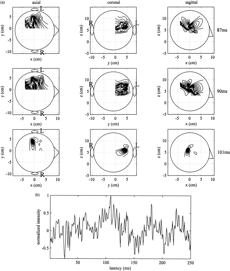
Results of applying the the minimum‐variance beamformer to the data shown in Figure 8. (a) Reconstructed source magnitude distributions at 87 msec (top row), 90 msec (middle row), and 101 msec (bottom row). (b) Estimated time course obtained at a location where the intensity in the results in Figure 9a has the maximum value.
Figure 11.
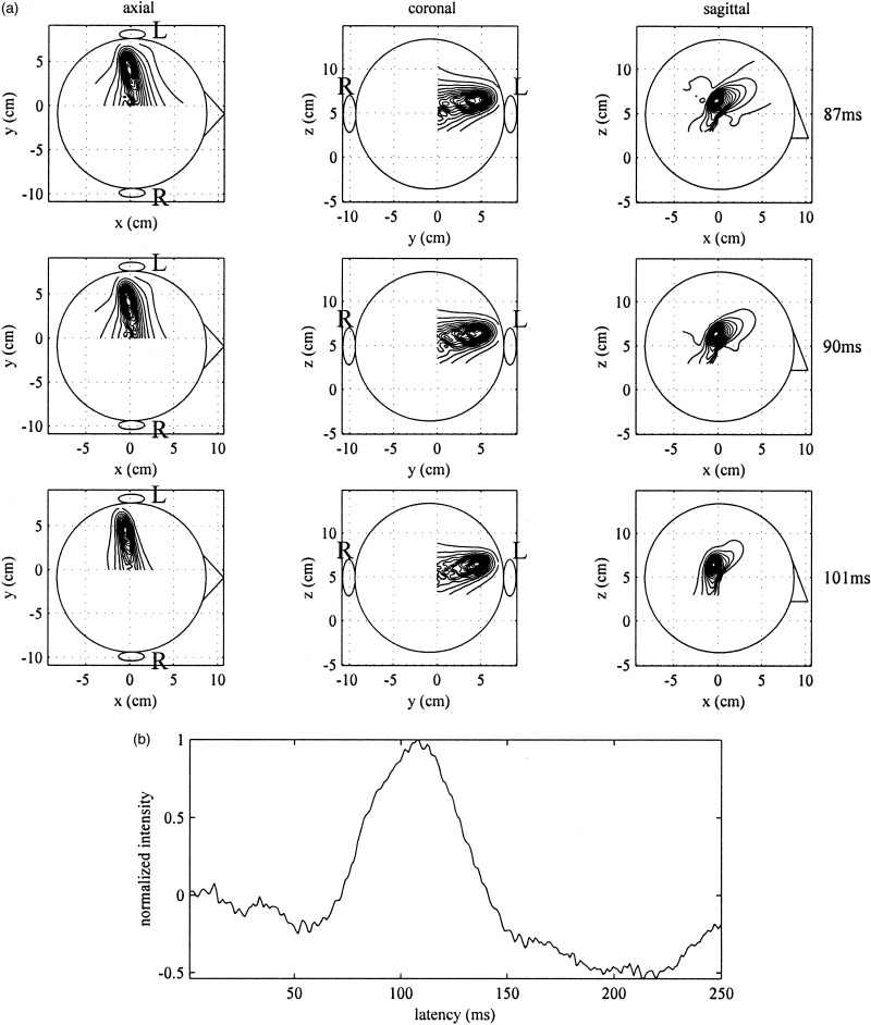
Results of applying the the minimum‐variance beamformer with the regularized inverse to the data shown in Figure 8. (a) Reconstructed source magnitude distributions at 87 msec (top row), 90 msec (middle row), and 101 msec (bottom row). (b) Estimated time course obtained at a location where the intensity in the results in (a) has the maximum value.
Results From Prewhitened Beamformer
We applied the prewhitened beamformer to the data set shown in Figure 12a. The data set was one of the 100‐epoch selectively averaged results obtained in a series of syllable‐discrimination experiments. The auditory stimuli used in the experiments were four kinds of syllables /dae/, /bae/, /pae/, and /tae/. The subject was asked to discriminate the voiced syllables /dae/ and /bae/ from the voiceless syllables /pae/ and /tae/. The subject pressed one response button when perceiving a /dae/ or /bae/ and pressed another button when perceiving a /pae/ or /tae/. Stimuli were presented to the subject's right ear, and the sensor array was placed above the subject's left hemisphere. The subject used his left fingers to press the response buttons. The four syllables were presented in a pseudo random order at a variable inter‐stimulus interval ranging from 1–1.5 sec. The averaged response for the particular syllable /bae/ are shown in Figure 12a. The activity in the motor area elicited by button pressing was roughly time locked to the stimulus and thus the influence from such a motor activity was contained to some extent in this auditory response despite that the subject used his epsi‐lateral fingers.
Figure 12.
Thirty‐seven channel recordings of an auditory magnetic field evoked by the voiced syllable /bae/. A total of 100 epochs were averaged. The two vertical broken lines indicate time instants at 78, 101 msec, at which the snapshots of the source activity are shown in Figures 13 and 14. (b) Prewhitened eigenvalue spectrum of R b obtained from the time window between 0 and 200 ms of the data set shown in (a).
We applied the prewhitened eigenspace beamformer to test its effectiveness in removing the influence of the motor activities. The measurement covariance matrix was calculated from the time window between 0–200 msec, and the noise covariance matrix was calculated from the time window between −100–0 msec (the whole prestimulus portion). The dimension of the signal subspace was set at 1 because the prewhitened eigenvalue spectrum (shown in Fig. 12b) contained one large eigenvalue. The reconstructed source‐magnitude maps for two time instants, 78 and 101 msec, are shown in Figure 13a; these time instants are shown by two vertical lines in Figure 12a. At both time instants, the activation in the primary auditory area was clearly detected by the proposed prewhitened beamformer. The results from the non‐prewhitened eigenspace‐based beamformer are shown in Figure 13b for comparison. The source reconstruction at 101 msec contains a single localized activity in the left primary auditory area. At the latency of 78 msec, however, the non‐prewhitened beamformer failed to detect the auditory source due, probably, to the existence of the background motor activity.
Figure 13.
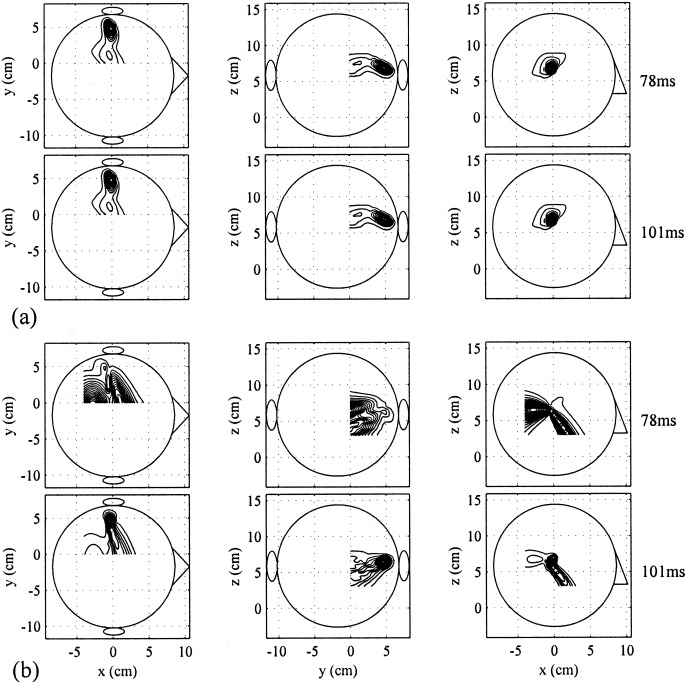
(a) Results of applying the prewhitened eigenspace‐based beamformer to the data shown in Figure 12a. Reconstructed source magnitude distributions at 78 msec (upper row) and 101 msec (bottom row). (b) Results of applying the non‐prewhitened eigenspace beamformer to the same data. Reconstructed source magnitude distributions at 78 msec (upper row) and 101 msec (bottom row).
DISCUSSION
In our numerical experiments the results of the spatio‐temporal reconstruction obtained by using the minimum variance beamformer was fairly noisy. In these experiments, the spherically homogeneous conductor model was used for both procedures: the generation of the simulated magnetic field and the forward calculation in the reconstruction. Therefore, the cause of such noisy reconstruction was primarily because of the use of the sample covariance matrix R̂ b. In our auditory experiments, because the spherically homogeneous conductor model was used for the forward calculation, the lead field matrix was not perfectly accurate and the primary cause of the noisy reconstruction is probably the use of such an inaccurate lead field in addition to the use of the sample covariance matrix. Therefore, these auditory experiments had very noisy results. A comparison among Figures 9, 10, 11 suggests that the use of the eigenspace‐based beamformer is highly effective for the spatio‐temporal reconstruction of source activities.
We emphasize, though, that the effectiveness of the eigenspace‐based beamformer becomes evident only when we perform spatio‐temporal reconstruction. For time‐averaged reconstruction, the results obtained using either the minimum variance or the eigenspace‐based beamformer were more or less the same (as shown by the time‐averaged reconstruction in Figs. 3 and 5). This is probably the reason why the poor performance of the minimum‐variance beamformer has been somewhat overlooked in the previous investigations [Robinson and Vrba, 1999; van Drongelen et al., 1996; van Veen et al., 1997]. In these investigations, the spatio‐temporal reconstruction of source activities was not emphasized; instead, a time‐averaged reconstruction of the source activities was obtained.
The signal subspace dimension Q in equation (8) is in principle determined by separating distinctly large eigenvalues from the small eigenvalues. This separation, however, may not be easy if there is no clear threshold in the eigenvalue spectrum. For example, the results in Figure 13a were obtained by setting the signal subspace dimension to one. This determination, however, is somewhat ambiguous because, as can be seen in Figure 12b, there are two more eigenvalues that are much smaller than the first eigenvalue but still greater than the noise‐level eigenvalues. The results obtained by setting the signal‐subspace dimension at three are shown in Figure 14. The comparison between Figures 13a and 14 shows that when the signal subspace dimension was determined differently, the final results were not significantly different.
Figure 14.
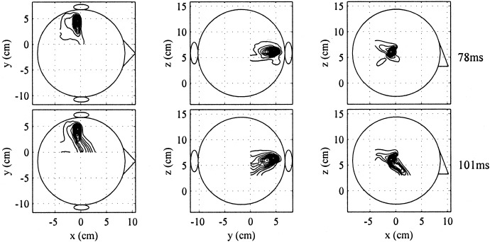
Results of applying the prewhitened eigenspace‐based beamformer to the data shown in Figure 12a with the signal subspace dimension set at 3.
In general, the overestimation of the signal subspace dimension gives intermediate results between those from the minimum‐variance beamformer and those from the eigenspace beamformer with a correct signal‐subspace dimension. Let us consider the case where the signal subspace dimension is overestimated at Q + Δ. Then, the SNR of such an eigenspace beamformer, SNRΔ is expressed as,
| (21) |
where
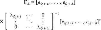 |
Because the relationship εTΓε<εTΓε holds, the relationship SNR(ES) > SNRΔ > SNR(MV) always holds true. Moreover, if εTΓε is small compared to εTΓε, the eigenspace‐based beamformer with an overestimated signal‐subspace dimension gives nearly the same SNR as that from the eigenspace‐based beamformer with a correct signal‐subspace dimension. The results in Figure 14 exactly show this case.
In summary, we have applied the eigenspace‐based beamformer to reconstruct spatio‐temporal activities of neural sources. This beamformer attains a SNR significantly higher than that of the minimum‐variance beamformer, particularly when errors in estimating the sensor lead field exist. We further extended the eigenspace beamformer so that it incorporates the information regarding the noise spatial correlation. The effectiveness of these eigenspace‐based beamformer techniques was validated in our numerical experiments and experiments using auditory responses.
Acknowledgements
The authors wish to thank Ms. Susanne Honma and Dr. Timothy Roberts for their help in performing auditory MEG measurements. This work was carried out as part of the MIT‐JST International Cooperative Research Project “Mind Articulation”. The work was also funded by a grant from the Whitaker Foundation to SN.
This appendix describes the method of obtaining a reasonable estimate of the source orientation. This method was used in our experiments. The source orientations can be obtained by utilizing the orthogonality relationship in equation (4). The optimum estimate of η is one that minimizes the following measure of this orthogonality;
| (22) |
This minimization problem can be solved by using the generalized‐eigenproblem formulation. The optimum orientation ηˆ opt ( r) satisfies the relationship,
| (23) |
where λmin indicates the minimum eigenvalue of this generalized eigenvalue problem. Therefore, the optimum estimate of the source‐moment orientation is obtained by finding the eigenvector corresponding to the minimum eigenvalues of equation (23).
When noise is non‐white and has a known covariance matrix, the orthogonality relationship is expressed in equation (19). The optimum orientation ηˆ opt(r) should therefore be obtained solving
| (24) |
That is, the eigenvector corresponding to the miminum eigenvalue λ˜min in the above equation gives the optimum estimate of the source‐moment orientation. The method presented in this appendix was originally developed for estimating the polarization of wavefronts received by an array of antennas in radar‐signal processing [Ferrara and Parks, 1983; Li, 1994; Schmidt, 1981], and its application to estimating an orientation of neuromagnetic sources has been reported [Mosher et al., 1992; Mosher and Leahy, 1998; Sekihara and Scholz, 1996].
Footnotes
REFERENCES
- Capon J (1969): High‐resolution frequency wavenumber spectrum analysis. Proc IEEE 57: 1408–1419. [Google Scholar]
- Carlson BD (1988): Covariance matrix estimation errors and diagonal loading in adaptive arrays. IEEE Trans Aerospace Electronic Syst 24: 397–401. [Google Scholar]
- Chang L, Yeh CC (1992): Performance of DMI and eigenspace‐based beamformers. IEEE Trans Antenn Propagat 40: 1336–1347. [Google Scholar]
- Chang L, Yeh CC (1993): Effect of pointing errors on the performance of the projection beamformer. IEEE Trans Antenn Propagat 41: 1045–1056. [Google Scholar]
- Cox H, Zeskind RM, Owen MM (1987): Robust adaptive beamforming. IEEE Trans Signal Process 35: 1365–1376. [Google Scholar]
- Feldman DD, Griffiths LJ (1991): A constrained projection approach for robust adaptive beamforming. Proceedings of the International Conference on Acoustics, Speech, and Signal Processing, Toronto. p 1357–1360.
- Ferrara ER, Parks TM (1983): Direction finding with an array of antennas having diverse polarizations. IEEE Trans Antenn Propagat 31: 231–236. [Google Scholar]
- Gross J, Ioannides AA (1999): Linear transformations of data space in MEG. Phys Med Biol 44: 2081–2097. [DOI] [PubMed] [Google Scholar]
- Hämäläinen M, Hari R, IImoniemi RJ, Knuutila J, Lounasmaa OV (1993): Magnetoence‐phalography‐theory, instrumentation, and applications to noninvasive studies of the working human brain. Rev Mod Phys 65: 413–497. [Google Scholar]
- Li J (1994): On polarization estimation using a crossed‐dipole array. IEEE Trans Signal Process 42: 977–983. [Google Scholar]
- Mosher JC, Lewis PS, Leahy RM (1992): Multiple dipole modeling and localization from spatio‐temporal MEG data. IEEE Trans Biomed Eng 39: 541–557. [DOI] [PubMed] [Google Scholar]
- Mosher JC, Leahy RM (1998): Recursive music: a framework for EEG and MEG source localization. IEEE Trans Biomed Eng 45: 1342–1354. [DOI] [PubMed] [Google Scholar]
- Richmond CD (1998): Response of sample covariance based MVDR beamformer to imperfect look and inhomogeneities. IEEE Signal Process Let 5: 325–327. [Google Scholar]
- Roberts TPL, Poeppel D, Rowley HA (1998): Magnetoencephalography and magnetic source imaging. Neuropsychiatry Neuropsychol Behav Neurol 11: 49–64. [PubMed] [Google Scholar]
- Robinson SE, Vrba J (1999): Functional neuroimaging by synthetic aperture magnetometry (SAM) In: Yoshimoto T, et al., editors. Recent advances in biomagnetism. Sendai: Tohoku University Press; p 302–305. [Google Scholar]
- Sarvas J (1987): Basic mathematical and electromagnetic concepts of the biomagnetic inverse problem. Phys Med Biol 32: 11–22. [DOI] [PubMed] [Google Scholar]
- Scharf LL (1991): Statistical signal processing: detection, estimation, and time series analysis, New York: Addison‐Wesley Publishing Co. 252 p. [Google Scholar]
- Schmidt RO (1981): A signal subspace approach to multiple emitter location and spectral estimation. PhD thesis. Stanford, CA: Stanford University.
- Sekihara K, Scholz B (1996); Generalized Wiener estimation of 3D current distribution from biomagnetic measurements In: Aine CJ, et al., editors. Biomag 96: Proceedings of the Tenth International Conference on Biomagnetism. New York: Springer‐Verlag; p 338–341. [Google Scholar]
- Sekihara K, Poeppel D, Marantz A, Koizumi H, Miyashita Y (1997): Noise covariance incorporated MEG‐MUSIC algorithm: a method for multiple‐dipole estimation tolerant of the influence of background brain activity. IEEE Trans Biomed Eng 44: 839–847. [DOI] [PubMed] [Google Scholar]
- Spencer ME, Leahy RM, Mosher JC, Lewis PS (1992): Adaptive filters for monitoring localized brain activity from surface potential time series. Conference record for 26th Annual Asilomer Conference on Signals, Systems, and Computers. p 156–161.
- van Drongelen W, Yuchtman M, van Veen BD, van Huffelen AC (1996): A spatial filtering technique to detect and localize multiple sources in the brain. Brain Topogr 9: 39–49. [Google Scholar]
- van Veen BD (1988): Eigenstructure based partially adaptive array design. IEEE Trans Antenn Propagat 36: 357–362. [Google Scholar]
- van Veen BD, Buckley KM (1988): Beamforming: a versatile approach to spatial filtering. IEEE ASSP Magazine 5: 4–24. [Google Scholar]
- van Veen BD, van Drongelen W, Yuchtman M, Suzuki A (1997): Localization of brain electrical activity via linearly constrained minimum variance spatial filtering. IEEE Trans Biomed Eng 44: 867–880. [DOI] [PubMed] [Google Scholar]
- Yu JL, Yeh CC (1995): Generalized eigenspace‐based beamformers. IEEE Trans Signal Process 43: 2453–2461. [Google Scholar]