

Abstract
This study aimed to characterize the neural generators of the early components of the visual evoked potential (VEP) to isoluminant checkerboard stimuli. Multichannel scalp recordings, retinotopic mapping and dipole modeling techniques were used to estimate the locations of the cortical sources giving rise to the early C1, P1, and N1 components. Dipole locations were matched to anatomical brain regions visualized in structural magnetic resonance imaging (MRI) and to functional MRI (fMRI) activations elicited by the same stimuli. These converging methods confirmed previous reports that the C1 component (onset latency 55 msec; peak latency 90–92 msec) was generated in the primary visual area (striate cortex; area 17). The early phase of the P1 component (onset latency 72–80 msec; peak latency 98–110 msec) was localized to sources in dorsal extrastriate cortex of the middle occipital gyrus, while the late phase of the P1 component (onset latency 110–120 msec; peak latency 136–146 msec) was localized to ventral extrastriate cortex of the fusiform gyrus. Among the N1 subcomponents, the posterior N150 could be accounted for by the same dipolar source as the early P1, while the anterior N155 was localized to a deep source in the parietal lobe. These findings clarify the anatomical origin of these VEP components, which have been studied extensively in relation to visual‐perceptual processes. Hum. Brain Mapping 15:95–111, 2001. © 2001 Wiley‐Liss, Inc.
Keywords: VEP, dipoles, MRI, fMRI, retinotopic mapping, V1, ERP, C1, co‐registration
INTRODUCTION
The neural generators of the early components of the pattern‐onset visual evoked potential (VEP) are not fully understood. Since the original observations of Jeffreys and Axford (1972a), many studies have obtained evidence that the first major VEP component (C1), with an onset latency between 40 and 70 msec and peak latency between 60 and 100 msec, originates from primary visual cortex (Brodmann's area 17, striate cortex). Several authors, however, have questioned this proposal and concluded that the C1 arises from extrastriate areas 18 or 19. Table I lists the conclusions of previous studies regarding the generators of the C1 component. Evidence that C1 is generated in the striate cortex within the calcarine fissure comes from studies showing that the C1 reverses in polarity for upper vs. lower visual‐field stimulation (e.g., Jeffreys and Axford, 1972a,b; Butler et al., 1987; Clark et al., 1995; Mangun, 1995). This reversal corresponds to the retinotopic organization of the striate cortex, in which the lower and upper visual hemifields are mapped in the upper and lower banks of the calcarine fissure, respectively. According to this “cruciform model” (Jeffreys and Axford, 1972a), stimulation above and below the horizontal meridian of the visual field should activate neural populations with geometrically opposite orientations and hence elicit surface‐recorded evoked potentials of opposite polarity. Such a pattern would not be observed for VEPs generated in other visual areas that lack the special retinotopic organization of the calcarine cortex, although it cannot be excluded that some degree of polarity shift for upper versus lower field stimuli might be present for neural generators in V2 and V3 as well (Schroeder et al., 1995; Simpson et al., 1994, 1995).
Table I.
Conclusions of previous studies regarding the cortical visual areas that generate the first (C1) and second (C2/P1) component of pattern‐onset VEP
| Authors | C1 | C2/P1 |
|---|---|---|
| Jeffreys and Axford, 1972a,b | 17 | 18 |
| Biersdorf, 1974 | 17 | 17 |
| Lesevre and Joseph, 1979 | 19 | 18 |
| Darcey and Arj, 1980 | 17 | 17 or 18 |
| Kriss and Halliday, 1980 | 17 | |
| Lesevre, 1982 | 17 | 18 |
| Parker et al., 1982 | 17 | |
| Butler et al., 1987 | 17 | |
| Maier et al., 1987 | 18 or 19 | 17 and 18 |
| Srebro, 1987 | 17 | |
| Edwards and Drasdo, 1987 | 18 | |
| Ossenblok and Spekreijse, 1991 | 18 | 19 |
| Bodis‐Wollner et al., 1992 | 17 | |
| Manahilov, et al., 1992 | 17 | 19 |
| Mangun et al., 1993 | 17 | 18 and 19 |
| Gomez Gonzalez, et al., 1994 | 17 | 18 and 19 |
| Clark et al., 1995 | 17 | 18 and 19 |
| Mangun, 1995 | 17 | 18 and 19 |
| Clark and Hillyard, 1996 | 17 | 18 and 18 |
| Miniussi et al., 1998 | 17 | 18 or 19 |
| Martinez et al., 1999 | 17 | 18 and 19 |
| Martinez et al., 2001a,b | 17 | 18 and 19 |
The second VEP component is a positivity termed P1 (called C2 by Jeffreys) with an onset latency between 65 and 80 msec and a peak latency of around 100 and 130 msec. There is evidence that this component, which does not show a polarity reversal for upper vs. lower visual‐field stimulation (Clark et al., 1995; Mangun, 1995), is mainly generated in extrastriate visual areas, although no clear consensus has yet been reached regarding the exact location of its sources (see Table I).
This lack of agreement among previous studies may be due to the low spatial resolution of the electrophysiological techniques employed and to methodological differences such as number of recording sites and type of stimuli used. In particular, a sparse electrode array may not able to differentiate concurrent activities in neighboring visual areas nor obtain an accurate picture of the voltage topography produced by a given source. Furthermore, the use of relatively large stimuli extending over wide visual angles in some studies might have activated widespread cortical areas, thereby reducing the possibility of identifying the exact generator locations. Finally, individual differences in the position and extent of the striate cortex with respect to the calcarine fissure (Rademacher et al., 1993) might have lead to variation among subjects in VEP topography.
The point of departure for the present research is the study of Clark et al. (1995), which used dipole modeling to localize the C1 component to the striate cortex and the P1 component to extrastriate areas 18/19. Clark et al. (1995) observed systematic changes in the orientation of the dipole corresponding to the C1 as function of stimulus polar angle (elevation) in the visual field that were in good agreement with the cruciform model. For stimuli in the lower visual field, however, they found it difficult to separate the voltage topography of the surface‐positive C1 from that of overlapping P1, perhaps due to the limited mapping resolution achieved with only a 32‐channel recording array. Accordingly, Clark et al. (1995) found it necessary to constrain the position of the C1 and P1 dipoles to observe the retinotopic polarity inversion of the C1.
The purpose of the present study was to separate the early C1 and P1 components and test their retinotopic properties with greater precision by using a denser electrode array (64‐channels recordings) and dipole modeling with no position constraints. In addition, the VEP sources localized by the dipole modeling were projected onto anatomical MRI sections and then compared to loci of cortical activations revealed by fMRI in response to the same stimuli. The stimuli used were flashed checkerboard patterns of relatively high spatial frequency to evoke a large C1 component (e.g., Martínez et al., 2001b; Rebaï et al., 1998). The stimuli were presented asymmetrically in the upper and lower quadrants of the visual fields to verify the polarity reversal of the C1 in light of evidence that the reversal point is not exactly at the horizontal meridian but rather at 10–20° (polar angle) below it (Aine et al., 1996; Clark et al., 1995). Thus, the overall goal was to determine the component structure and source localization of the early (60–160 msec) VEP using combined electrophysiology and fMRI techniques.
MATERIALS AND METHODS
Subjects
Twenty‐three paid volunteer subjects (12 female, mean age 26.1, range 18–36 years) participated in the VEP recordings. A subset of 13 of these subjects (8 female, mean age 26.8 range 23–35 years) additionally received anatomical MRI scans. Of the latter group, a subset of five subjects (3 female, mean age 27.3, range 19–35 years) also participated in the fMRI study. All subjects were right‐handed and had normal or corrected‐to‐normal visual acuity.
Stimuli
The stimuli consisted of circular checkerboards sinusoidally modulated in black and white; each stimulus had a diameter of 2° of visual angle and a spatial frequency modulation of 4 cycles per degree. These stimuli were flashed for 50 msec duration against a gray background (20 cd/m2) that was isoluminant with the mean luminance of the checkerboard pattern, which itself was modulated at a contrast of 80%. In the VEP experiment, stimuli were presented binocularly one at a time in randomized sequences to the four quadrants of the left and right visual fields at a fast rate (SOAs varying between 250 and 550 msec). Stimulus positions were centered along an arc that was equidistant (4°) from a central fixation point and located at polar angles of 25° above and 45° below the horizontal meridian (Fig. 1). These asymmetrical positions were chosen so that the upper and lower field stimuli would stimulate approximately the opposite zones of the lower and upper banks of the calcarine fissure, respectively, based on findings that the horizontal meridian its actually represented on the lower bank rather than at the lateral recess of the calcarine fissure (Aine et al., 1996; Clark et al., 1995).
Figure 1.
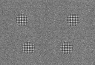
Stimuli used in this experiment. Circular sinusoidal checkerboards were flashed one at time in random order to the four locations.
In the fMRI experiment the same stimuli were presented at the same locations and rate, but the stimuli were delivered in 20‐sec blocks to one quadrant a time instead of in random order.
Procedure
In the VEP experiment, the subject was comfortably seated in a dimly lit sound‐attenuated and electrically shielded room while stimuli were presented on a video monitor at a viewing distance of 70 cm. Subjects were trained to maintain stable fixation on a central dot (0.2°) throughout stimulus presentation. Each run lasted 100 sec followed by a 30 sec rest, with longer breaks interspersed. A total of 24 runs were carried out to deliver 1,400 stimuli to each quadrant. To maintain alertness during stimulation, in both the VEP and fMRI experiments subjects were required to press a button upon detection of an infrequent and difficult to detect brightness change of the fixation dot. The subjects were given feedback on their behavioral performance and their ability to sustain fixation. The fMRI experiment consisted of five runs of 6 min each, with each quadrant receiving stimulation in successive 20 sec intervals.
Electrophysiological Recording and Data Analysis
The EEG was recorded from 62 scalp sites using the 10‐10 system montage (Nuwer et al, 1999). Standard 10‐20 sites were FP1, FPz, FP2, F7, F3, Fz, F4, F8, T7, C3, Cz, C4, T8, P7, P3, Pz, P4, P8, O1, Oz, O2, and M1. Additional intermediate sites were, AF3, AFz, AF4, FC5, FC3, FC1, FCz, FC2, FC4, FC6, C5, C1, C2, C6, TP7, CP5, CP3, CP1, CPz, CP2, CP4, CP5, TP8, P5, P1, P2, P6, PO7, PO3, POz, PO4, PO8, I5, I3, Iz, I4, I6, SI3, SIz, and SI4. All scalp channels were referenced to the right mastoid (M2). Horizontal eye movements were monitored with a bipolar recording from electrodes at the left and right outer canthi. Blinks and vertical eye movements were recorded with an electrode below the left eye, which was also referenced to the right mastoid.
The EEG from each electrode site was digitized at 250 Hz with an amplifier bandpass of 0.1 to 80 Hz (half amplitude low‐ and high‐frequency cutoffs, respectively) together with a 60 Hz notch filter and was stored for off‐line averaging. Computerized artifact rejection was performed before signal averaging to discard epochs in which deviations in eye position, blinks, or amplifier blocking occurred. In addition, epochs that were preceded by a target stimulus (fixation point task) within 1,000 msec or followed within 500 msec were eliminated to avoid contamination of the average by VEPs related to target detection and motor response. On average, about 12% percent of the trials were rejected for violating these artifact criteria. Blinks were the most frequent cause for rejection.
VEPs to the checkerboards stimuli were averaged separately according to stimulus position in each of the four quadrants. To further reduce high‐frequency noise, the averaged VEPs were low‐pass filtered at 46 Hz by convolving the waveforms with a gaussian function.
fMRI Scanning
Subjects were selected for participation in fMRI scanning on the basis of their ability to maintain steady visual fixation as assessed by electro‐oculographic recordings during the VEP recording sessions. Stimuli were back‐projected onto a screen inside the magnet bore and were viewed via a mirror.
Functional imaging was carried out on a Siemens VISION 1.5T clinical scanner equipped with gradient echo‐planar capabilities and a standard‐equipment polarized flex surface coil optimized for brain imaging. Blood oxygen level dependent (BOLD) images were acquired with an echo planar imaging sequence (TR = 2,500 msec, TE = 64 msec, flip angle = 90°) in the coronal plane (4 × 4 mm in‐plane resolution). One hundred forty repetitions on each of 15 4 mm slices were acquired during each six‐minute run; the first two repetitions were not used in the data analysis. Imaging began at the occipital pole and extended anteriorly.
For anatomical localization, high‐resolution (1 × 1 × 1 mm) T1‐weighted images of the whole brain were acquired using a 3‐D magnetization prepared rapid gradient echo sequence (TR = 11.4 msec, TE = 4.4 msec, flip angle = 10°). Both anatomical and BOLD‐weighted images were transformed into the standardized coordinate system of Talairach and Tournoux (1988).
Time‐dependent echo‐planar images were post‐processed with AFNI software (Cox, 1996). After 3D motion correction, the raw time series data from each run were averaged within each individual. Group data were obtained by averaging the raw time series data over all subjects. A series of phase‐shifted trapezoids representing the periodic alternation of conditions in the block design of the experiment (i.e., stimulus presentation at the four positions) was used as the reference waveform. Each trapezoid function was correlated on a pixel‐by‐pixel basis with the averaged (individual or group) signal strength time series by a least squares fit to generate a functional activation map. Gram‐Schmitt orthogonalization was used to remove linear drift in the time series.
Retinotopic visual areas were mapped in three subjects using the method of Sereno et al. (1995). Polar angle (angle from the center‐of‐gaze) was mapped on the cortical surface using a rotating wedge of flickering checks; eccentricity (distance from the center‐of‐gaze) was mapped using an expanding ring of flickering checks. From these paired scans field‐sign maps were generated to delineate the borders of retinotopically organized visual areas based on whether they contain a mirror‐image, or non‐mirror image representation of the visual field. In the present study, the retinotopic maps for each subject were based on the average of at least four scans (two mapping polar angle and two mapping eccentricity; 12,480 functional images in total).
Modeling of VEP Sources
A Polhemus spatial digitizer was used to record the 3D coordinates of each electrode and of three fiducial landmarks (the left and right preauricular points and the nasion). A computer algorithm was used to calculate the best‐fit sphere that encompassed the array of electrode sites and to determine their spherical coordinates. The mean spherical coordinates for each site averaged across all subjects were used for the topographic mapping and source localization procedures. In addition, individual spherical coordinates were related to the corresponding digitized fiducial landmarks and to fiducial landmarks identified on the whole‐head MRIs of 13 subjects. In this manner, the locations of the estimated dipoles could be related to individual brain‐skull anatomy.
Maps of scalp voltage were obtained (Perrin et al., 1989) for the VEPs to stimuli at each of the four spatial positions. Estimation of the dipolar sources of early VEP components was carried out using Brain Electrical Source Analysis (BESA version 2.1) The BESA algorithm estimates the location and the orientation of multiple equivalent dipolar sources by calculating the scalp distribution that would be obtained for a given dipole model (forward solution) and comparing it to the original VEP distribution. Interactive changes in the location and in the orientation in the dipole sources lead to minimization of the residual variance (RV) between the model and the observed spatio‐temporal VEP distribution (Scherg, 1990). The energy criterion of the BESA was set at 15% to reduce the interaction among dipoles and the separation criterion was set at 10% to optimize the separation of the source waveforms that differ over time. In these calculations, BESA assumed an idealized three‐shell spherical head model with the radius obtained from the average of the twenty‐three subjects (89.6 mm), and the scalp and skull thickness of 6 and 7 mm, respectively. Single dipoles or pairs were fit sequentially over specific latency ranges (given below) to correspond with the distinctive components in the waveform. Dipoles accounting for the earlier portions of the waveform were left in place as additional dipoles were added. The reported dipole fits were found to remain consistent as a function of starting position.
To estimate the positions of the dipole sources with respect to brain anatomy and fMRI activations, the dipole coordinates calculated from the group average VEP distributions were projected onto the MRIs of individual subjects (Anllo‐Vento et al., 1998; Clark and Hillyard, 1996; Giard et al., 1994; Pantev et al., 1995). The line between the anterior (A) and the posterior (P) commissures was identified on each subject's MRI scan as the principal A‐P axis for the Talairach and Tournoux (1988) system, and the 3D coordinates of each dipole in the group average BESA model were determined on the MRI with respect to the Talairach axes, scaled according to brain size. The mean values of these individual Talairach coordinates of each dipole were calculated over the 13 subjects and were taken as estimate of the average anatomical position of each dipole generator source across the group (Clark and Hillyard, 1996).
RESULTS
VEP Waveforms
The spatio‐temporal structure of the VEPs to stimuli in each of the four quadrants is shown in Figures 2 and 3. The major components are shown in expanded waveforms in Figure 4, and their amplitudes, latencies and topographic properties are listed in Table II.
Figure 2.
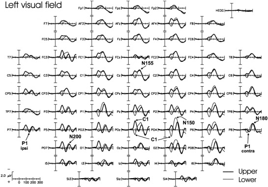
Grand average VEPs to stimuli located in the upper (thick line) and lower (thin line) quadrants of the left visual field.
Figure 3.
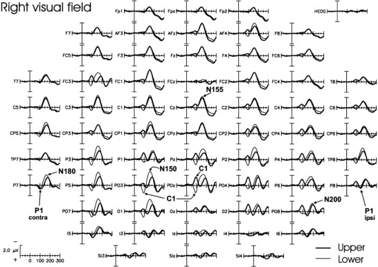
Same as in Figure 2 for the right visual field.
Figure 4.
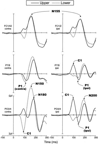
Grand average VEPs in response to upper (solid line) and lower hemifield (dashed line) stimuli. Waveforms are collapsed across VEPs to left and right hemifield stimuli and are plotted separately for scalp sites contralateral (left) and ipsilateral (right) to the side of stimulation.
Table II.
Topography, amplitudes (μV) and latencies (ms) of VEP components observed in this study*
| Component | Stimulus position | Topography | Electrodes used for measurement | Peak amplitude | Peak latencya | Dipole |
|---|---|---|---|---|---|---|
| C1 | Upper | Ipsilateral | PO3/PO4 | −1.6 | 92 (93) | 1 |
| Lower | Contralateral | PO3/PO4 | 1.9 | 90 (88) | 1 | |
| Early P1 | Upper | Contralateral | PO7/PO8 | 0.9 | 110 (108) | 2‐3 |
| Lower | Contralateral | P7/P8 | 1 | 98 (95) | 2‐3 | |
| Late P1 | Upper | Ipsilateral | PO3/PO4 | 0.8 | 146 (142) | 3‐2 |
| Lower | Ipsilateral | PO3/PO4 | 0.6 | 136 (137) | 3‐2 | |
| N150 | Lower | Contralateral | PO3/PO4 | −3.3 | 148 (148) | 2‐3 |
| N155 | Upper | Contralateral | FC1/FC2 | −1.5 | 156 (155) | 6‐7 |
| Lower | Contralateral | FC1/FC2 | −1.6 | 154 (156) | 6‐7 | |
| N180 | Upper | Contralateral | P7/P8 | −1.4 | 182 (178) | 2‐3‐4‐5 |
| Lower | Contralateral | P7/P8 | −1.6 | 178 (179) | 4‐5 | |
| N200 | Upper | Ipsilateral | PO3/PO4 | −1.3 | 200 (198) | 3‐2 |
| Lower | Ipsilateral | PO3/PO4 | −1.6 | 192 (194) | 3‐2 |
Measurements were made at indicated recording sites for VEPs to contralateral or ipsilateral stimuli. Peak latencies and amplitudes were averaged over VEPs to stimuli in left and right visual fields.
Latencies in parentheses refer to mean latency of peaks in source waveforms of indicated dipoles.
The earliest component (C1) had an average onset latency of about 55 msec and a peak latency of 90–92 msec. For upper field stimuli the C1 was most prominent at midline and ipsilateral occipito‐parietal sites, and for lower field stimuli the C1 was largest at midline and contralateral occipito‐parietal sites. In all subjects, the C1 varied systematically in polarity as a function of stimulus position, being negative for stimuli in the upper fields and positive for the stimuli in the lower fields.
Overlapping in time with the C1, the early phase of the P1 component was elicited at contralateral occipito‐temporal sites. This component had an average onset latency of 72–80 msec and peak latency of 110 msec for the upper fields (98 msec for the lower fields). These latency differences are most likely attributable to overlap with the polarity inverting C1. The P1 did not change in polarity and varied little in amplitude for stimuli in the upper versus lower hemifields. A later phase of the P1 was elicited at ipsilateral occipito‐temporal sites with a mean onset latency of 110–120 msec and peak latency of 146 msec for the upper fields (136 msec for the lower fields). This component did not vary appreciably in polarity or amplitude between the four spatial positions.
In the interval between 140 and 200 msec, several negative waves were elicited concurrently at different scalp locations. This complex of spatially and temporally overlapping waves is often referred to collectively as the N1 component, but here the subcomponents will be labeled according to their approximate peak latencies. The first negative peak (N150) was elicited primarily by lower field stimuli at contralateral occipito‐parietal sites. A second negative component (N155) was prominent at contralateral frontal‐central sites, while a third component (N180) was distributed over contralateral temporo‐parietal sites. Finally, a fourth negative component (N200) was present at ipsilateral occipito‐parietal sites. These latter three components did not change appreciably in latency or amplitude for stimuli at the four spatial positions.
VEP Topography
Figures 5 and 6 show the voltage topographies of the five major components in the first 160 msec of the VEP waveform. In the 70–85 msec interval the C1 was negative and maximal in amplitude between the occipito‐parietal midline and the ipsilateral sites for the upper field stimuli. For the lower field stimuli, C1 amplitude was positive and maximal between the occipito‐parietal midline and the contralateral sites. The contralateral P1 at 95–115 msec was largest over occipito‐temporal sites; its polarity remained positive for upper and lower quadrant stimuli, although its focus was situated more superiorly for stimuli in the lower fields. During the interval 120–140 msec the ipsilateral P1 focus can be seen, and both the ipsilateral and contralateral P1 positivity during this interval was more broadly and inferiorly distributed than in the 95–115 msec range. The beginning of the occipito‐parietal N150 was also evident during this interval in response to lower field stimuli. Finally, the N155 was broadly distributed over the frontal‐central scalp with a contralateral predominance during the 140–160 msec interval.
Figure 5.
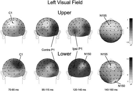
Spline‐interpolated voltage maps of VEP components elicited by LVF stimuli in the latency range of C1 (70–85 msec), early P1 (95–115 msec), late P1 (120–140) and N1 (140–160 msec) components.
Figure 6.
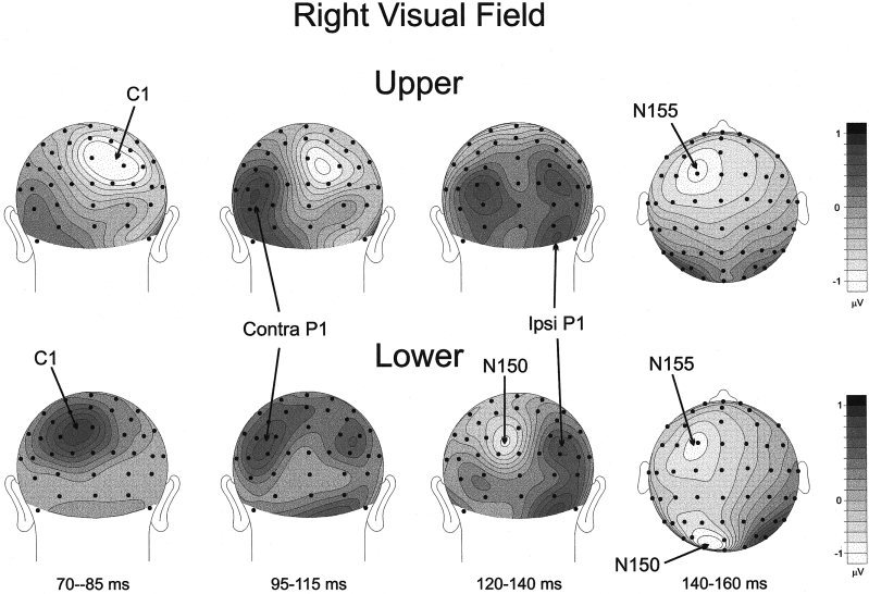
Same as in Figure 5 except for the RVF.
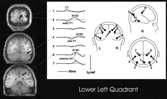
Dipole Modeling
Inverse dipole modeling of the early VEP components in the time range 64–160 msec was carried out on the grand average waveforms using the BESA algorithm. Separate dipole models were calculated for each of the four quadrants (Fig. 7). The C1 distributions were fit in the 64–84 msec time interval with a single dipole (1) that was located in medial occipital cortex, slightly contralateral to the midline; the dipoles for the upper quadrants were situated slightly lower than for the lower quadrants. For the upper quadrants, the C1 dipoles had their negative poles oriented superiorly, posteriorly and ipsilaterally. In contrast, for the lower quadrants the C1 dipoles were oriented with their negative poles pointing inferiorly, anteriorly and ipsilaterally. In the saggital plane, the C1 dipoles for the upper and lower quadrants showed an inversion in orientation of about 180°.
Figure 7.
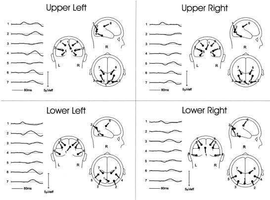
BESA dipole models fitted to the grand‐average VEPs to stimuli in the four visual field quadrants. Waveforms at the left of each model show the time course of source activity for each of the modeled dipoles. Dipole 1 corresponds to the C1 component, dipole pair 2‐3 to the early P1, dipole pair 4‐5 to the late P1, and dipole pair 6‐7 to the N155.
The early, contralateral phase of P1 was fit over 80–110 msec with a pair of symmetrical dipoles (2, 3) that were situated in dorsal occipital cortex; dipoles for the upper quadrants were slightly inferior to those for the lower quadrants. The positive pole of the P1 dipoles was oriented contralaterally for the upper quadrants. For the lower quadrants, the positive pole was oriented more posteriorly and superiorly. The source waveforms in Figure 7 show that the contralateral early P1 dipole accounts for the positivity in the 80–110 msec range whereas the ipsilateral dipole accounts for a later positivity. In addition, the contralateral dipole well accounts for the N150 elicited by lower field stimuli
The later phase of P1 that included both ipsilateral and contralateral foci was fit over the interval 110–140 msec with a pair of symmetrical dipoles (4, 5) that were located in ventral occipital cortex. The dipoles were situated more laterally and orientated more contralaterally for lower than for upper quadrant stimuli.
The anteriorly distributed N155 was fit over the interval 130–160 msec with a pair of symmetrical dipoles (6, 7) that were situated deep in the parietal lobe, medial to the intraparietal sulcus and lateral to the cingulate sulcus. The negative poles of the N155 dipoles were oriented contralaterally, anteriorly and superiorly for all quadrants.
These multi‐dipole models each accounted for more than 98% of the variance in scalp voltage topography for each quadrant over the time range 64–160 msec (see Table III for residual variance values and dipole coordinates). Because of the multiplicity of dipoles needed to fit the 64–160 msec range, no attempt was made here to add additional dipoles to account for the later N180 and N200 subcomponents. It can be seen in the source waveforms of Figure 7, however, that N180 and N200 activity is accounted for by both the early and late P1 dipoles.
Table III.
Locations and orientations of BESA fitted dipoles expressed in Talairach coordinates*
| X | Y | Z | |
|---|---|---|---|
| Upper Left | |||
| C1 | 7 | −81 | 10 |
| Early P1 | ±29 | −84 | 7 |
| Late P1 | ±35 | −46 | −15 |
| N155 | ±17 | −39 | 38 |
| RV = 1.79% | |||
| Upper Right | |||
| C1 | −6 | −82 | 10 |
| Early P1 | ±30 | −85 | 8 |
| Late P1 | ±35 | −44 | −13 |
| N155 | ±20 | −36 | 38 |
| RV = 1.28% | |||
| Lower Left | |||
| C1 | 9 | −86 | 14 |
| Early P1 | ±34 | −85 | 14 |
| Late P1 | ±37 | −41 | −10 |
| N155 | ±18 | −36 | 37 |
| RV = 1.81% | |||
| Lower Right | |||
| C1 | −7 | −92 | 12 |
| Early P1 | ±35 | −83 | 13 |
| Late P1 | ±39 | −40 | −18 |
| N155 | ±20 | −33 | 40 |
| RV = 1.97% | |||
Values are in mm. Residual variance (RV) is the percentage of variability not explained by the model.
Anatomical Localization
Sensory‐evoked fMRI activations were observed in multiple visual cortical areas in the hemisphere contralateral to the stimulated visual field (see Table IV). These areas included the calcarine fissure, the lingual and fusiform gyri, the middle occipital gyrus and its neighboring sulci, and the parietal cortex. There was a close correspondence between the fMRI activations in the calcarine and middle occipital areas and the dipole coordinates of the C1 and early P1 components, respectively (compare Tables III and IV). For the late P1 the correspondence was less precise, with the dipole positions situated from 13–19 mm anterior to the center of the mean fMRI activations in the fusiform gyrus. These fusiform activations generally extended from 10–20 mm along the anterior‐posterior axis, however, and hence the anterior borders of the active zones were closely adjacent to the late P1 dipole position (e.g., see Fig. 11 below). The correspondence between the dipoles fit to the N155 and the neighboring fMRI activations in the parietal cortex varied among the quadrants, with separations ranging from 10–25 mm. It should be noted, however, that the N155 dipole positions were situated slightly anteriorly to the most anterior plane imaged with fMRI in some subjects, so that more anterior sites of activation may have contributed to N155 generation.
Table IV.
Mean values (over 5 subjects) of three‐dimensional Talairach coordinates of the striate and extrastriate activation sites in the fMRI experiment*
| X | Y | Z | |
|---|---|---|---|
| Upper Left | |||
| Striate | 10 | −78 | 3 |
| Mid. occ. | 31 | −82 | 11 |
| Fusiform | 29 | −59 | −16 |
| Parietal | 11 | −36 | 45 |
| Upper Right | |||
| Striate | −4 | −81 | 5 |
| Mid. occ. | −30 | −86 | 7 |
| Fusiform | −28 | −62 | −9 |
| Parietal | −8 | −46 | 46 |
| Lower Left | |||
| Striate | 13 | −85 | 10 |
| Mid. occ. | 31 | −82 | 17 |
| Fusiform | 33 | −56 | −8 |
| Parietal | 30 | −48 | 47 |
| Lower Right | |||
| Striate | −8 | −90 | 6 |
| Mid. occ. | −29 | −81 | 17 |
| Fusiform | −34 | −59 | −14 |
| Parietal | −8 | −48 | 56 |
Values are in mm.
Figure 11.
Spatial correspondence between dipole models fitted to the grand average VEP and fMRI activations in a single subject (KD). fMRI activations and retinotopic mappings of visual areas for upper and lower right field stimuli were projected onto a flattened cortical representation of the left hemisphere. Dashed white lines represent the boundaries of visual areas traced from visual field sign maps (sulcal cortex, dark gray; gyral cortex, light gray). Coronal and saggital sections display the same activations before flattening. The circles with pointers indicate the fitted dipoles from the grand‐average VEP model in response to the same stimuli.
Figure 8 shows areas of significant activation in the image planes corresponding to the C1 dipole for upper field stimuli in two representative subjects. Note that a zone of activation in the calcarine fissure corresponds closely to the location of the C1‐fitted dipole. The individual variation (across subjects) in the correspondence between the calcarine activations and the grand average C1 dipoles is shown in Figure 9 in Talairach space. For each quadrant of stimulation, the centers of fMRI activations (small circles) were found to cluster around the calculated position of the corresponding C1 dipole (large circle with pointer).
Figure 8.
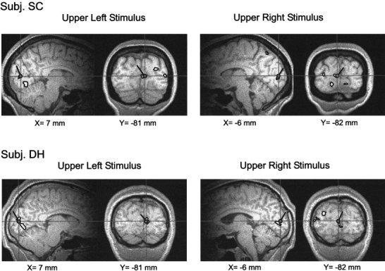
Spatial correspondence between dipole models fitted to the grand average VEP for the C1 component (circle with pointer) and sites of activation in calcarine fissure shown by fMRI in response to the same stimuli in two individual subjects.
Figure 9.
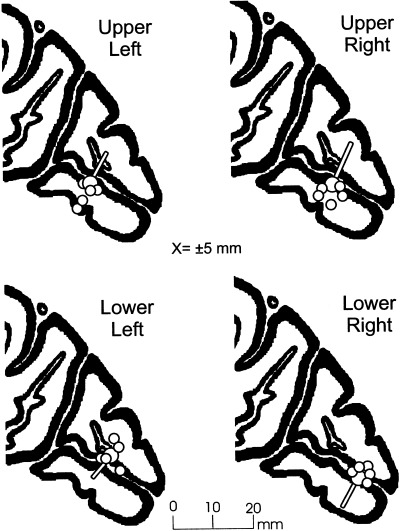
Anatomical correspondence between the modeled dipoles for the C1 component (large circles with pointers) and sites of activation in the calcarine fissure shown by fMRI (small circles) in response to the same stimuli in 5 individual subjects. In these saggital views both the dipole positions and the centers of calcarine activation are shown in Talairach space.
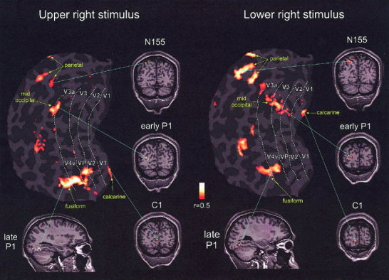
Figure 10 illustrates for one quadrant the generally good correspondence between the mean fMRI activations in several cortical areas and the modeled dipoles, as follows: calcarine, C1; lateral mid‐occipital, early P1; ventral fusiform, late P1; deep parietal, anterior N155.
Figure 10.
Spatial correspondence between dipole models fitted to the grand‐average VEP and sites of activation in the grand‐average fMRI in response to stimuli in the lower left quadrant. For the late P1 and N155 the dipole locations were situated anteriorly to the plane of the MRI/fMRI section by 15 and 8 mm, respectively. See Tables III and IV for data from all 4 quadrants.
To localize the stimulus‐evoked fMRI activations with respect to the retinotopically organized visual areas, the visual area boundaries were defined on the basis of their calculated field signs (Sereno et al., 1995). Using this method, the borders of retinotopically organized visual areas (V1, V2, V3, VP, V3a, and V4v) were identified in three subjects, and activations in striate and adjacent extrastriate visual areas could be distinguished despite their close proximity and despite individual differences in cortical anatomy. Figure 11 shows the fMRI activations in one subject in response to upper and lower right field stimulation superimposed on the flattened cortical surface. These same activations and the corresponding fitted dipoles are also shown on coronal and saggital sections. The C1 dipole corresponds closely with the V1 activation, whereas the early P1 dipole is colocalized with activations in areas V3/V3a and adjacent middle‐occipital gyrus. The late P1 dipole corresponds with the anterior portion of the extended V4v/fusiform gyrus activations. The N155 dipole was localized medially with respect to a site of activation in the intraparietal sulcus. These relationships were consistently observed across the four quadrants in the three subjects studied with retinotopic mappings: for upper field stimuli there were loci of activation in the ventral mappings of V1 and V2, in VP, V4v, and in an anterior adjacent region of the fusiform gyrus that may correspond to the upper field representation of area V8 (Hadjikhani et al., 1998; Tootell et al., 2001; Wandell, 1999); for lower field stimuli activations were found in the upper mappings of V1 and V2, in V3, V3a, and in an anterior adjacent area that may correspond the lower field representation of V7 (Tootell et al., 1998, 2001). For both upper and lower field stimuli there were similar loci of activation in parietal sites adjacent to or within the intraparietal sulcus.
DISCUSSION
The present results provide strong support for the hypothesis that the first major component of the VEP elicited by a pattern onset stimulus (C1) arises from surface‐negative activity in the primary visual cortex (human analogue of V1, area 17). The scalp topography of the C1, its short onset latency (55 msec), retinotopic polarity inversion, and dipole source modeling in conjunction with structural and functional MRI all point to a neural generator in area V1 within the calcarine fissure. This conclusion is in accordance with the findings of a number of previous studies (see Table I), but the present experiment is the first to our knowledge to provide converging evidence from functional neuroimaging in support of a striate cortex generator.
The scalp distribution of the C1 component showed maximal amplitudes at parieto‐occipital sites and could be distinguished from the spatially and temporally overlapping P1 component by its more medial distribution and its greater sensitivity to the retinotopic position of the stimuli. For all subjects, the C1 showed an inversion in polarity in response to changes in stimulus position between upper and lower quadrants in accordance with the cruciform model of primary visual cortex. This inversion was verified by dipole modeling that showed a near 180° rotation of the C1's dipole for upper vs. lower field stimuli.
The present dipole modeling also found the C1 source to be localized within the calcarine fissure for both upper and lower field stimuli. In a previous modeling study (Clark et al., 1995), the dipole representing the C1 was localized to the calcarine area for upper field stimuli, but for lower field stimuli an anomalous ventral occipital localization was obtained. This was evidently a consequence of failure to separate the overlapping positive C1 and P1 distributions during modeling with a limited electrode array (30 scalp sites). Thus, to demonstrate a retinotopic polarity inversion of the C1, Clark et al. (1995) had to constrain the position of the C1 dipole to the same location for upper and lower field stimulation. In the present study, however, the 64‐channel array was evidently adequate to separate the C1 and P1 distributions, and the C1 was localized to calcarine cortex for stimuli in all quadrants without any need for position constraints.
Further evidence supporting a striate generator for the C1 component came from projecting its estimated dipole locations on high‐resolution structural MRI images along with corresponding fMRI activations. Anatomical localization of the C1 dipole corresponded closely with the sites of fMRI activation in the calcarine fissure elicited by the same stimuli positioned at the same locations of the visual field. Retinotopic mapping of individual subject's visual areas using the method of Sereno et al. (1995) confirmed that both dipolar sources of the C1 component and the fMRI activation loci were located within primary visual cortex (area V1).
The source modeling carried out here separated the subsequent positive deflection (P1) into early (80–110 msec) and late (110–140 msec) phases, based on differences in timing and scalp distribution. For stimuli in all quadrants, the early P1 dipole was localized to lateral extrastriate cortex (area 18), whereas the late P1 dipole was estimated to lie in ventral occipito‐temporal cortex. These dipole positions correspond well with fMRI activations in and adjacent to the middle occipital gyrus and the posterior fusiform gyrus, respectively. By placing these fMRI activations for individual subjects on mappings of their retinotopic visual‐cortical areas, the early P1 dipole was found to correspond with activations in areas V3, V3a, and adjacent middle occipital gyrus and the late P1 dipole with activations anterior to area V4 in the fusiform gyrus. These dipole positions for P1 are in general agreement with those of previous VEP (Clark et al., 1995; Clark and Hillyard, 1996; Martínez et al., 2001) and MEG (Aine et al., 1995; Portin et al., 1999; Supek et al., 1999) studies. Although it is difficult to match components between VEP and MEG studies, Supek et al. (1999) found the visual‐evoked MEG activity between 80–170 msec could be modeled by three sources; one in the calcarine area and two extrastriate sources in dorsal occipito‐parietal and ventral occipito‐temporal areas, respectively. These sources may overlap with those proposed here for the C1, early P1, and late P1 components, respectively.
The N1 complex of negative components in the 150–200 msec range arises from a multiplicity of generators that has proven difficult to analyze. Previous attempts to account for the N1 complex with only one or two pairs of dipoles (e.g., Clark et al., 1995; Clark and Hillyard, 1996) resulted in obvious oversimplifications. In the present analysis the N1 was decomposed into four temporally overlapping subcomponents (N150, N155, N180, and N200). The occipital N150 was well accounted for by the contralateral early P1 dipole for lower field stimuli, and the anterior N155 by a pair of centro‐parietal dipoles. No attempt was made here to fit dipoles to the time intervals of the N180 and N200 components due to the burgeoning complexity of the model for the earlier components, but it is evident from the sources waveform of Figures 7 and 10 that much N180 activity is accounted for by the contralateral early and late P1 dipoles and N200 activity by the ipsilateral P1 dipoles. The present analysis cannot be regarded as definitive, however, and future studies should examine the possibility of more anterior sources beyond the fMRI planes that were examined here.
It should be noted that the use of hemodynamic imaging to substantiate the estimated locations of ERP sources, as was done in the present and previous (Heinze et al., 1994; Mangun et al., 2001; Martínez et al., 1999, 2001a; Snyder et al., 1995) studies, is subject to certain caveats. First and foremost is the assumption that the hemodynamic response obtained with fMRI or PET is colocalized with the same neural activity that gives rise to the ERP. With regard to visual‐evoked activity, such colocalization appears to be optimal for human medial occipital cortex (including the calcarine fissure) and is less clear for extrastriate visual areas (Gratton et al., 2001). These observations may help explain why the colocalizations observed here between the C1 dipole and fMRI activations in area V1 were more precise than those between P1/N1 dipoles and the extrastriate activations. Other factors may also play a role, however, such as a more accurate dipole model for the initial C1 component than for subsequent VEP components that receive contributions from multiple temporally and spatially overlapping cortical generators.
CONCLUSION
The present analysis combined VEP recording with structural and functional MRI and retinotopic mapping of visual cortical areas to support the hypothesis that the initial VEP component (C1) arises from neural generators in primary visual cortex whereas the subsequent P1 and N1 components are generated in multiple extrastriate cortical areas. These findings extend previous studies of the multiple sources of the pattern‐onset VEP and provide more precise information about the anatomical origins of cortical activity patterns that have been related to visual perception and attention in previous reports. For example, the present data linking the C1 to a striate cortex generator, together with previous findings that this component is not modulated as function of selective attention (Clark and Hillyard, 1996; Gomez‐Gonzales et al., 1994; Mangun, 1995; Martínez et al., 1999, 2001a, 2001b; Wijers et al., 1997), considerably strengthen the hypothesis that attentional mechanisms first influence visual processing at a level beyond the initial evoked response in area V1. These results also lend support to proposals that neural activity in area V1 is not sufficient to produce conscious visual experience (e.g., Crick and Koch, 1995). On the other hand, the present results, together with evidence that the later P1 and N1 components are modulated as function of visual attention and perception (e.g., Heinze et al., 1990; Hillyard and Anllo‐Vento, 1998; Luck et al., 1994; Mangun, 1995; Mangun and Hillyard, 1990), provide a basis for linking these perceptual processes with neural activity in specific extrastriate visual areas.
REFERENCES
- Aine CJ, Supek S, George JS (1995): Temporal dynamics of visual‐evoked neuromagnetic sources: effects of stimulus parameters and selective attention. Int J Neurosci 80: 79–104. [DOI] [PubMed] [Google Scholar]
- Aine CJ, Supek S, George JS, Ranken D, Lewine J, Sanders J, Best E, Tiee W, Flynn ER, Wood CC (1996): Retinotopic organization of human visual cortex: departures from the classical model. Cereb Cortex 6: 354–361. [DOI] [PubMed] [Google Scholar]
- Anllo‐Vento L, Luck SJ, Hillyard SA (1998): Spatio‐temporal dynamics of attention to color: evidences from human electrophysiology. Hum Brain Mapp 6: 216–238. [DOI] [PMC free article] [PubMed] [Google Scholar]
- Biersdorf WR (1974): Cortical evoked responses from stimulation of various regions of the visual field. Doc Ophthalmol Proc 3: 247–259. [Google Scholar]
- Bodis‐Wollner I, Brannan JR, Nicoll J, Frkovic S, Mylin LH (1992): A short latency cortical component of the foveal VEP is revealed by hemifield stimulation. Electroencephalogr Clin Neurophysiol 84: 201–208. [DOI] [PubMed] [Google Scholar]
- Butler SR, Georgiou GA, Glass A, Hancox RJ, Hopper JM, Smith KR (1987): Cortical generators of the C1 component of the pattern‐onset visual evoked potential. Electroencephalogr Clin Neurophysiol 68: 256–267. [DOI] [PubMed] [Google Scholar]
- Clark V, Hillyard SA (1996): Spatial selective attention affects early extrastriate but not striate components of the visual evoked potential. J Cogn Neurosci 8: 387–402. [DOI] [PubMed] [Google Scholar]
- Clark VP, Fan S, Hillyard SA (1995): Identification of early visually evoked potential generators by retinotopic and topographic analysis. Hum Brain Mapp 2: 170–187. [Google Scholar]
- Cox RW (1996): AFNI: software for analysis and visualization of functional magnetic resonance neuroimages. Comput Biomed Res 29: 162–173. [DOI] [PubMed] [Google Scholar]
- Crick F, Koch C (1995): Are we awake of neural activity in primary visual cortex? Nature 375: 121–123. [DOI] [PubMed] [Google Scholar]
- Darcey TM, Arj JP (1980): Spatio‐temporal visually evoked scalp potentials in response to partial‐field patterned stimulation. Electroencephalogr Clin Neurophysiol 50: 348–355. [DOI] [PubMed] [Google Scholar]
- Edwards L, Drasdo N (1987): Scalp distribution of visual evoked potentials to foveal pattern and luminance stimuli. Doc Ophthalmol 66: 301–311. [DOI] [PubMed] [Google Scholar]
- Giard MH, Perrin F, Echallier JE, Thevenet M, Froment JC, Pernier J (1994): Dissociation of temporal and frontal components in the human auditory N1 wave: a scalp current density and dipole model analysis. Electroencephalogr Clin Neurophysiol 92: 238–252. [DOI] [PubMed] [Google Scholar]
- Gomez‐Gonzalez CM, Clark VP, Fan S, Luck SJ, Hillyard SA (1994): Sources of attention‐sensitive visual event‐related potentials. Brain Topogr 7: 41–51. [DOI] [PubMed] [Google Scholar]
- Gratton G, Goodman‐Wood MR, Fabiani M (2001): Comparison of neuronal and hemodynamic measures of the brain response to visual stimulation: an optical imaging study. Hum Brain Mapp 13: 13–25. [DOI] [PMC free article] [PubMed] [Google Scholar]
- Hadjikhani N, Liu AK, Dale AM, Patrick Cavanagh P, Tootell R (1998): Retinotopy and color sensitivity in human visual cortical area V8. Nat Neurosci 1: 235–241. [DOI] [PubMed] [Google Scholar]
- Heinze HJ, Mangun GR, Hillyard SA (1990): Visual event‐related potentials index perceptual accuracy during spatial attention to bilateral stimuli In: Brunia C, Gallard A, Kok A, editors. Psychophysiological brain research. The Netherlands: Tilburg University Press; p 196–202. [Google Scholar]
- Heinze HJ, Mangun GR, Burchert W, Hinrichs H, Scholz M, Münte TF, Gös A, Johannes S, Scherg M, Hundeshagen H, Gazzaniga MS, Hillyard SA (1994): Combined spatial and temporal imaging of spatial selective attention in humans. Nature 392: 543–546. [DOI] [PubMed] [Google Scholar]
- Hillyard SA, Anllo‐Vento L (1998): Event‐related brain potentials in the study of visual selective attention. Proc Natl Acad Sci USA 95: 781–787. [DOI] [PMC free article] [PubMed] [Google Scholar]
- Jeffreys DA, Axford JG (1972a): Source locations of pattern‐specific component of human visual evoked potentials. I. Component of striate cortical origin. Exp Brain Res 16: 1–21. [DOI] [PubMed] [Google Scholar]
- Jeffreys DA, Axford JG (1972b): Source locations of pattern‐specific component of human visual evoked potentials. II. Component of extrastriate cortical origin. Exp Brain Res 16: 22–40. [DOI] [PubMed] [Google Scholar]
- Kriss A, Halliday AM (1980): A comparison of occipital potentials evoked by pattern onset, offset, and reversal In: Barber C, editor. Evoked potentials. Lancaster, UK: UMP Press; p 205–212. [Google Scholar]
- Lesevre N (1982): Chronotopographical analysis of the human evoked potential in relation to the visual field (data from normal individuals and hemianopic patients). Ann NY Acad Sci 388: 156–182. [DOI] [PubMed] [Google Scholar]
- Lesevre N, Joseph JP (1979): Modifications of pattern‐evoked potential (PEP) in relation to the stimulated part of the visual field (clues for the most probable origin of each component). Electroencephalogr Clin Neurophysiol 47: 183–203. [DOI] [PubMed] [Google Scholar]
- Luck SJ, Hillyard SA, Mouloua M, Woldorff MG, Clark VP, Hawkins HL (1994): Effect of spatial cuing on luminance detectability: psychophysical and electrophysiological evidence for early selection. J Exp Psychol Hum Percept Perform 20: 1000–1014. [DOI] [PubMed] [Google Scholar]
- Maier J, Dagnelie G, Spekreijse H, van Dijk BW (1987): Principal component analysis for source localization VEPs in man. Vision Res 27: 165–177. [DOI] [PubMed] [Google Scholar]
- Manahilov V, Riemslag FC, Spekreijse H (1992): The Laplacian analysis of the pattern onset response in man. Electroencephalogr Clin Neurophysiol 82: 220–224. [DOI] [PubMed] [Google Scholar]
- Mangun GR, Hillyard SA (1990): Allocation of visual attention on spatial locations: tradeoff function for event‐related brain potential and detection performance. Percept Psychophys 47: 532–550. [DOI] [PubMed] [Google Scholar]
- Mangun GR, Hillyard SA, Luck SJ (1993): Electrocortical substrates of visual selective attention In: Meyer DE, Kornblum S, editors. Attention and performance XIV: synergies in experimental psychology, artificial intelligence, and cognitive neuroscience. Cambridge, MA: MIT Press; p 219–243. [Google Scholar]
- Mangun GR (1995): Neural mechanisms of visual selective attention. Psychophysiology 32: 4–18. [DOI] [PubMed] [Google Scholar]
- Mangun GR, Hinrichs H, Scholz M, Mueller‐Gaertner HW, Herzog H, Krause BJ, Tellman L, Kemna L, Heinze HJ (2001): Integrating electrophysiology and neuroimaging of spatial selective attention to simple isolated visual stimuli. Vision Res 41: 1423–1435. [DOI] [PubMed] [Google Scholar]
- Martínez A, Anllo‐Vento L, Sereno MI, Frank LR, Buxton RB, Dubowitz DJ, Wong EC, Hinrichs H, Heinze HJ, Hillyard SA (1999): Involvement of striate and extrastriate visual cortical areas in spatial attention. Nat Neurosci 2: 364–369. [DOI] [PubMed] [Google Scholar]
- Martínez A Di Russo F, Anllo‐Vento L, Sereno MI, Buxton RB, Hillyard SA (2001a): Putting spatial attention on the map: timing and localization of stimulus selection processes in striate and extrastriate visual areas. Vision Res 41: 1437–1457. [DOI] [PubMed] [Google Scholar]
- Martínez A, Di Russo F, Anllo‐Vento L, Hillyard SA (2001b): Electrophysiological analysis of cortical mechanisms of selective attention to high and low spatial frequencies. Clin Neurophysiol. [DOI] [PubMed] [Google Scholar]
- Miniussi C, Girelli M, Marzi CA (1998): Neural site of redundant target effect: electrophysiological evidence. J Cogn Neurosci 10: 216–230. [DOI] [PubMed] [Google Scholar]
- Nuwer MR, Lehmann D, da Silva FL, Matsuoka S, Sutherling W, Vibert JF (1999): IFCN guidelines for topographic and frequency analysis of EEGs and EPs. The International Federation of Clinical Neurophysiology. Electroencephalogr Clin Neurophysiol 52(Suppl): 15–20. [PubMed] [Google Scholar]
- Ossenblok P, Spekreijse H (1991): The extrastriate generators of EP to checkerboard onset. A source localization approach. Electroencephalogr Clin Neurophysiol 80: 181–193. [DOI] [PubMed] [Google Scholar]
- Pantev C, Bertrand O, Eulitz C, Verkindt C, Hampson S, Schuierer G, Elbert T (1995): Specific tonotopic organizations of different areas of the human auditory cortex revealed by simultaneous magnetic and electric recordings. Electroencephalogr Clin Neurophysiol 94: 26–40. [DOI] [PubMed] [Google Scholar]
- Parker DM, Salzen EA, Lishman JR (1982): The early wave of the visual evoked potential to sinusoidal gratings: responses to quadrant stimulation as a function of spatial frequency. Electroencephalogr Clin Neurophysiol 53: 427–435. [DOI] [PubMed] [Google Scholar]
- Perrin F, Pernier J, Bertrand O, Echallier JE (1989): Spherical splines for scalp potentials and current density mapping. Electroencephalogr Clin Neurophysiol 72: 184–187. [DOI] [PubMed] [Google Scholar]
- Portin K, Vanni S, Virsu V, Hari R (1999): Stronger occipital cortical activation to lower than upper visual field stimuli. Exp Brain Res 124: 287–294. [DOI] [PubMed] [Google Scholar]
- Rademacher J, Caviness VS Jr, Steinmetz H, Galaburda AM (1993): Topographical variation of the human primary cortices: implications for neuroimaging, brain mapping, and neurobiology. Cereb Cortex 3: 313–329. [DOI] [PubMed] [Google Scholar]
- Rebaï M, Bernard C, Lannou J, Jouen F (1998): Spatial frequency and right hemisphere: an electrophysiological investigation. Brain Cogn 36: 21–29. [DOI] [PubMed] [Google Scholar]
- Scherg M (1990): Fundamental of dipole source analysis In: Grandori F, Hoke M, Romani GL, editors. Auditory evoked magnetic fields and electric potentials. Basel: Karger; p 40–69. [Google Scholar]
- Schroeder CE, Steinschneider M, Javitt DC, Tenke CE, Givre SJ, Mehta AD, Simpson GV, Arezzo JC, Vaughan HG Jr (1995): Localization of ERP generators and identification of underlying neural processes. Electroencephalogr Clin Neurophysiol 44(Suppl): 55–75. [PubMed] [Google Scholar]
- Sereno MI, Dale AM, Reppas JB, Kwong KK, Belliveau JW, Brady TJ, Rosen BR, Tootell RB (1995): Borders of multiple visual areas in humans revealed by functional magnetic resonance imaging. Science 268: 889–893. [DOI] [PubMed] [Google Scholar]
- Simpson GV, Foxe JJ, Vaughan HG Jr, Mehta AD, Schroeder CE (1994): Integration of electrophysiological source analyses MRI and animal models in the study of visual processing and attention. Electroencephalogr Clin Neurophysiol 44(Suppl) 76–93. [PubMed] [Google Scholar]
- Simpson GV, Pflieger ME, Foxe JJ, Ahlfors SP, Vaughan HG Jr, Hrabe J, Ilmoniemi RJ, Lantos G (1995): Dynamic neuroimaging of brain function. J Clin Neurophysiol 12: 432–449. [DOI] [PubMed] [Google Scholar]
- Srebro R (1987): The topography of scalp potentials evoked by pattern pulse stimuli. Vision Res 6: 901–914. [DOI] [PubMed] [Google Scholar]
- Snyder AZ, Abdullaev YG, Posner MI, Raichle ME (1995): Scalp electrical potentials reflect regional cerebral blood flow responses during processing of written words. Proc Natl Acad Sci USA 92: 1689–1693. [DOI] [PMC free article] [PubMed] [Google Scholar]
- Supek S, Aine CJ, Ranken D, Best E, Flynn ER, Wood CC (1999): Single vs. paired visual stimulation: superposition of early neuromagnetic responses and retinotopy in extrastriate cortex in humans. Brain Res 830: 43–55. [DOI] [PubMed] [Google Scholar]
- Talairach J, Tournoux P (1988): Co‐planar stereotaxic atlas of the human brain. New York, NY: Thieme. [Google Scholar]
- Tootell RB, Mendola JD, Hadjikhani NK, Ledden PJ, Liu AK, Reppas JB, Sereno MI, Dale AM (1997): Functional analysis of V3A and related areas in human visual cortex. J Neurosci 17: 7060–7078. [DOI] [PMC free article] [PubMed] [Google Scholar]
- Tootell RB, Hadjikhani N, Hall EK, Marrett S, Vanduffel W, Vaughan JT, Dale AM (1998): The retinotopy of visual spatial attention. Neuron 21: 1409–1422. [DOI] [PubMed] [Google Scholar]
- Tootell RB, Hadjikhani NK (2001): Where is ‘dorsal V4’in human visual cortex? Retinotopic, topographic and functional evidence. Cereb Cortex 11: 298–311. [DOI] [PubMed] [Google Scholar]
- Wandell BA (1999): Computational neuroimaging of human visual cortex. Ann Rev Neurosci 22: 145–173. [DOI] [PubMed] [Google Scholar]
- Wijers AA, Lange JJ, Mulder G, Mulder LJ (1997): An ERP study of visual spatial attention and letter target detection for isoluminant and nonisoluminant stimuli. Psychophysiology 34: 553–565. [DOI] [PubMed] [Google Scholar]