

Abstract
Commonly used frameworks for spatial normalization of brain imaging data (e.g., Talairach‐space) are based on one or more adult brains. As pediatric brains are different in size and shape from adult brains and continue to develop through childhood, we aimed to assess the influence of age on various spatial normalization parameters. One hundred forty‐eight healthy children aged 5–18 years were included in this study. The linear scaling parameters and the deformations from the non‐linear spatial normalization to both a standard adult and a custom pediatric template were analyzed within SPM99. The effect of using a brain mask on the linear and of using different levels of constraint on the non‐linear spatial normalization was assessed. Of the linear scaling factors, only the X‐dimension (left–right) showed a significant age‐correlation when based on brain tissue, whereas the overall scaling was not correlated with age. When based on the whole head, a very strong age‐effect can be found in all dimensions. Non‐linear deformations also show localized correlations with age, most pronounced in parietal and frontal areas. The total amount of volume change is significantly lower when using a pediatric template. It is also substantially influenced by the degree of regularization that is exerted on the spatial normalization parameters. Our results suggest that in the cortical areas showing a strong correlation of deformation with age, caution should be used in assigning imaging results in children to a specific morphological structure. Also, to minimize the amount of deformation during non‐linear spatial normalization, a pediatric template should be used. Further implications of our findings on developmental neuroimaging studies are discussed. Hum. Brain Mapping 17:48–60, 2002. © 2002 Wiley‐Liss, Inc.
Keywords: spatial normalization, template, stereotaxic space, functional imaging, developmental neuroimaging
INTRODUCTION
Due to the individual variability in brain morphology, imaging data has to be spatially normalized to allow for inter‐individual comparison. This is achieved by transforming the individual image into a standardized stereotaxic space [Toga and Thompson, 2001]. This procedure provides a common spatial framework for describing functional activation or morphological changes. It makes group comparisons possible, which not only increases signal to noise ratio and statistical power, but also allows for the extrapolation of findings to the population as a whole [Grachev et al., 1999; Woods et al., 1998]. There have been several different approaches to spatial frameworks, the most widely used being the one described by Talairach and Tournoux [1988], based on data from one 60‐year‐old female. Later approaches used larger collections of normal brains and suggested other spatial dimensions [Collins et al., 1998; Mazziotta et al., 1995].
Normalization procedures can be divided into two main categories. Linear approaches do a purely affine transformation by finding the best combination of global translation, rotation, and scaling factors to transform a brain into a standardized stereotaxic space (global spatial normalization). In addition, higher‐order, non‐linear approaches may be used to match the source image to a template (or target) image on a regional level (regional spatial normalization), using different mathematical approaches [Thompson et al., 2000b]. Their common goal is to apply algorithms that minimize the differences between the source and the target image(s). Although spatial normalization was initially achieved by only a global transformation, recent approaches suggested additional regional non‐linear transformations to achieve a better fit of image and template [Ashburner and Friston, 1999; Kochunov et al., 2000; Thompson et al., 2000b].
There is some controversy about the applicability of a common framework in general and the most widely used framework, Talairach‐space [Talairach and Tournoux, 1988], in particular [Ashburner and Friston, 1999; Brett et al., 2001]. Despite the increasingly widespread use of spatial normalization, however, surprisingly few attempts have been made to assess the accuracy of this procedure. These include studies in which the authors manually defined landmarks and compared the “normalized” locations after applying spatial normalization procedures [Arndt et al., 1996; Dzemidzic et al., 1999]. Grachev et al. [1999] manually defined 256 landmarks and compared two different spatial normalization algorithms. Due to the lack of a gold standard in spatial transformation, however, the assessment of the actual registration accuracy is highly difficult [Woods et al., 1998]. This is especially true as the observed differences are “a combination of inter‐subject variations in identification of the landmark by the neuroradiologist and those from spatial registration error.” [Dzemidzic et al., 1999].
Spatial normalization in children poses special problems [Muzik et al., 2000; Toga and Thompson, 2001] as pediatric brains differ in size, composition and shape from adult brains [Casey et al., 2000; Courchesne et al., 2000]. This is especially relevant because the most widely used spatial normalization schemes incorporate information based on adult brain data. The question of the applicability of adult brain templates for the spatial normalization of pediatric brain image data is of great importance to those doing neuroimaging studies in children. One recent study already tried to address this question within SPM96 in a group of 13 children with epilepsy. Muzik et al. [2000] determined the deviation of children's outer brain contours compared to adult's brains after spatial normalization to a standard adult template. The authors found more variable outer contours in children than in adults; this effect was age‐dependent. They concluded that spatial normalization to an adult template is feasible in children 6 years or older [Muzik et al., 2000]. Apart from using a small group of patients with a neurological disorder, however, only a global measure of “deviation from adult contours” is given, and thus no inference about the location of changes can be made. Also, the spatial normalization algorithms and templates underwent major revisions and improvements for the current version of SPM (SPM99) used here and elsewhere [Ashburner and Friston, 1999, 2000; Gaser et al., 1999, 2001], making comparisons with recent and future publications difficult. Only one spatial normalization procedure was applied in all patients, precluding inferences on the possible influence of different spatial normalization procedures or on the contributions of linear and non‐linear components.
We address the question of a possible age‐dependence of different spatial normalization strategies in normal children. Due to the variability in determining landmarks and the ensuing uncertainties in ascribing the results, we chose to apply an almost completely automated image analysis procedure using SPM99. We aimed to assess a possible influence of age on both the affine and the non‐linear spatial normalization. The effect of the respective main regulatory influences (using a brain mask for the affine transformation and constraining the energy cost function of the non‐linear deformation) and the effect of using a custom‐made pediatric vs. a standard adult template should also be evaluated.
MATERIALS AND METHODS
Subject selection
Healthy children were recruited as part of an ongoing study on normal language development [Holland et al., 2001]. Institutional review board approval and informed consent were obtained for all subjects. Subjects were recruited from the community via television broadcasts and information flyers. Exclusion criteria were: history of previous neurological illness, head trauma with loss of consciousness, current or past psychostimulant medication, learning disability, IQ less than 80 (measured by the Wechsler Intelligence Scale for Children, Third Edition), birth at 37 weeks or less of gestational age, pregnancy, abnormal findings on clinical neurological examination, and clinical or technical contraindications to an MRI‐examination (including orthodontic braces). A qualified pediatric neuroradiologist read all MRI scans for structural abnormalities.
Image acquisition
Children were imaged with a Bruker Biospec 30/60 3T MRI scanner equipped with a head gradient insert (Bruker SK330). A whole‐brain, T1‐weighted modified driven‐equilibrium Fourier transform (MDEFT) [Ugurbil et al., 1993] image was acquired (TR = 15 msec, TE = 4.3 msec, τ‐time = 550 msec, flip angle = 20°, matrix = 128 × 256 × 96, FOV = 19.2 × 25.6 × 14.4 cm, resolution = 1.5 × 1 × 1.5 mm).
Data pre‐processing
All of the automated image processing was done using statistical parametrical mapping software (SPM99, Wellcome Department of Cognitive Neurology, University College London, UK) [Friston et al., 1995] running in MATLAB (MathWorks, Natick, MA) unless otherwise stated. Further calculations were done using stand‐alone MATLAB‐scripts and customized IDL‐programs (Research Systems International, Boulder, CO).
As the single manual step in image preparation and analysis, determination of the anterior commissure was performed by a single investigator for all images. During this procedure, images were also carefully aligned along the main axes to correct for grossly different head positions in the scanner, providing optimal starting estimates for the subsequent spatial normalization procedures. In addition to the manual alignment, the effect of differing head positions (pose) was subsequently further minimized in the original deformation using a Procrustes procedure [Bookstein, 1997] as described in Ashburner [2000]. The procedure yields a transformation matrix, which was processed as described below. The scans were rated (regarding the presence of arterial blood flow‐artifacts and motion artifacts) on a scale from 0 (no flow or motion artifact) to 4 (strong flow or motion artifact). Images with a rating of 3 or 4 were excluded from further analysis. The remaining high‐quality images (n = 148) were reoriented in the axial plane and resliced to 1 × 1 × 1 mm isotropic voxels to reduce partial volume effects in further processing and to achieve a better fit with the axially oriented templates. As in all of the other processing steps within SPM99, a sinc‐interpolation algorithm was used when possible. Images were in neurological orientation, thus avoiding flipping during spatial normalization.
Construction of a pediatric template
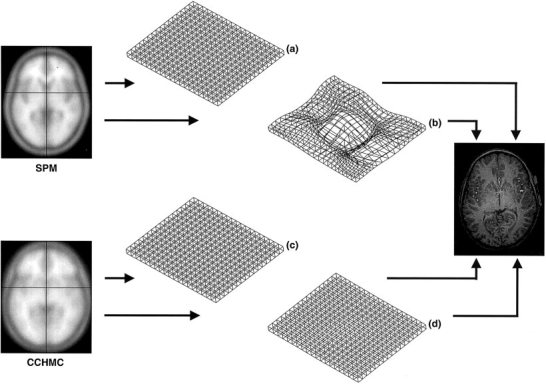
To address the possible difference pertaining to the use of a standard adult template during non‐linear transformation, a custom pediatric template was constructed first from all high‐quality images. These were automatically transformed into stereotaxic space within SPM99 by a 12‐parameter affine‐only, linear transformation to avoid regional distortion of the images ([1] in Fig. 1). All images were then averaged and written out as one template image. A corresponding, pediatric brain mask was also created. By modeling smoothly varying intensity changes, residual image inhomogeneities were removed [Ashburner and Friston, 2000]. This procedure involves the estimation of an intensity nonuniformity field, which is then applied to the image to remove these nonuniformities, yielding an image corrected for these nonuniformities. The function modulating the nonuniformity is forced to be smooth to avoid fitting higher‐frequency variations caused by tissue type differences rather than field nonuniformities. The image was (according to SPM‐template specifications) smoothed with an 8 mm Gaussian kernel to facilitate fitting [Ashburner et al., 1997]. This template will be referred to as the CCHMC‐template (Cincinnati Children's Hospital Medical Center; ([2] in Fig. 1).
Figure 1.

Steps in data processing and analysis.
The affine transformation into a standard stereotaxic space [Mazziotta et al., 1995] was done twice, once with and once without using a brain mask that weighs the spatial normalization parameters on brain tissue as opposed to simply scaling the whole head. Because it was found that omitting brain masking introduced a strong age effect (see Results), a brain mask was used in the template construction and all following spatial normalization procedures.
Data processing
Images were also spatially normalized using the full‐scale automated spatial normalization procedure integrated in SPM99. In two separate procedures, either the standard T1‐weighted SPM99‐template ([3] in Fig. 1) or the custom CCHMC‐template ([2] in Fig. 1) was used as the target for non‐linear transformations. Here, the initial 12‐parameter affine transformation was followed by 16 non‐linear iterations using 8 × 8 × 8 discrete cosine transform basis functions. These aim at minimizing both the sum of squared differences between image and template and the energy cost function of this transformation [Ashburner and Friston, 1999, 2000]. To further describe the characteristics of these deformations, the parameter responsible for the constraint of this energy cost function was set to two values (“high” or “low regularization”). The parameters of these four transformations (SPMLOW, SPMHIGH, CCHMCLOW and CCHMCHIGH) were automatically saved and used in further analyses ([4] in Fig. 1). See Figure 1 for all the steps in data processing and analyses.
Determination of affine parameters
The linear scaling factors of the affine transformation were determined from the 12‐parameter affine transformation matrix. The three parameters in the transformation resulting from simple translation were discarded, leaving a 3 × 3 matrix whose eigenvalues are equal to the linear scaling factors. A combined scaling factor was obtained from the product of the three scaling factors. This factor is equivalent to the overall volume change attributable to linear scaling.
Determination of non‐linear deformations
The processed deformation was then presented as one image volume by computing and displaying the Jacobian determinants for each voxel. Images were written out in 2 × 2 × 2 mm resolution. In these images, the pixel intensity corresponds to the volume change this pixel underwent during spatial normalization (>1 = volume enlargement or <1 = volume reduction, with values closer to 1 indicating a smaller volume change) [Gaser et al., 1999]. Consequently, the volume of a region is decreased during spatial normalization for determinants greater than one, which means that the region is larger than the corresponding region in the template. This deformation maps from the spatially normalized to the un‐normalized image, it therefore represents the effect of both linear scaling and nonlinear deformations. The Jacobian determinant of an affine transformation will be a constant value over the whole volume as all voxels are scaled by the same factor, however, and thus undergo the same volume change. This fact was taken advantage of when removing the effect of the affine transformation from the original deformation, which was achieved by modulating the deformation with the individual (combined) linear scaling factor (including the [very small] scaling that occurred during the Procrustes procedure). This procedure yields images that represent the effect of non‐linear deformations only ([4] in Fig. 1).
The final images were smoothed with a Gaussian kernel (full width at half maximum [FWHM] = 8 mm) to create a local weighted average of the surrounding pixels. Due to the matched filter theorem, the width of the smoothing kernel determines the scale at which changes are most sensitively detected [White et al., 2001]. This step also renders the data more normally distributed, which increases the validity of the following statistical tests [Ashburner and Friston, 2000].
Image analysis and statistics
The processed images from all four datasets (SPMLOW, SPMHIGH, CCHMCLOW, and CCHMCHIGH) were analyzed within SPM99, employing the framework of the general linear model [Friston et al., 1995]. A model was designed in which age (in months at date of examination) was used as the covariate of interest, whereas gender (due to its significant influence on brain structure) [Giedd et al., 1996] was used as a covariate of no interest. Two contrasts were calculated, testing for a positive or negative correlation of the value of the Jacobean determinant with the parameter of interest (age). Significance was set at a P‐value of P = 0.05, corrected for multiple comparisons, and an additional extent threshold of 25 voxels. Although the strictness of the P‐value‐correction has been questioned and less rigid corrections were recently proposed [Genovese et al., 2001], this level of significance was chosen to ensure the display of only very strong, age‐related differences. Significance was not based on spatial extent as this (at least in the analysis of structural data) has been shown to increase the rate of false positives [Ashburner and Friston, 2000].
Data visualization
The linear scaling factors were plotted versus age to show their correlation with age. Significant results from the analysis of the non‐linear deformations were rendered on the standard SPM‐surface or on the CCHMC‐brain surface, excluding data from >10 mm outside of the brain. This pediatric brain surface was derived from segmentation data from the dataset used in making the CCHMC‐template.
To further characterize and visualize the total amount of volume change during non‐linear spatial normalization, the image intensity attributable to volume increases and volume decreases was determined separately for all pixels in the brain. This number represents the overall amount of (negative or positive) volume change in the brain during non‐linear spatial normalization.
To assess the distortions three‐dimensionally, the transformation of one child (the one with the median age, a boy of 131.38 months) was visualized for a single slice of 10 mm thickness (Z: −5/5). This was intended as a visualization tool to demonstrate the different effects of the non‐linear transformations in a specific example. Also, one cluster that was found to be present in all of the SPM/CCHMC‐datasets (parietal; * in Fig. 3) was analyzed in all datasets to exemplify its spatial extent.
Figure 3.

Correlation of volume change during non‐linear spatial normalization with age: significant positive (red, indicating an increase of the Jacobean Determinant in older children) and negative correlation (green, indicating a decrease of the Jacobean Determinant in older children) in the SPM‐ and CCHMC‐datasets. Results are rendered on the corresponding brain surfaces. P = 0.05, corrected for multiple comparisons. Extent threshold = 25 voxels. *Cluster summarized in Table II.
RESULTS
Subjects and scans
Overall, 200 children were examined. Data from 52 children was rejected due to insufficient quality, technical failure, or pathological findings, leaving data from 148 children (79 girls, 53.4%; 69 boys, 46.6%). Average age was 135.87 ± 41.9 months (11.32 ± 3.49 years), median = 131 months (10.92 years), range 60–226.5 months (5–18.87 years) at the date of the MR‐exam. The age and gender breakdown of this sample is given in Table I. Ethnic origin: Caucasian, 132; African‐American, 6; Asian, 5; Multi‐Ethnic, 2; Hispanic, 2; and Native American, 1. All but 15 children were right‐handed.
Table I.
Subject age and gender breakdown
| Age | |||||||
|---|---|---|---|---|---|---|---|
| 5–6 | 7–8 | 9–10 | 11–12 | 13–14 | 15–16 | 16–17 | |
| Female | 5 | 15 | 19 | 11 | 13 | 8 | 8 |
| Male | 8 | 16 | 13 | 14 | 9 | 3 | 6 |
Affine scaling parameters
When using a brain mask, only the scaling in the X‐dimension (left–right) showed a correlation with age (P = 0.03), whereas the other scaling factors showed no correlation with age (P = 0.12 [Y], P = 0.70 [Z]; solid symbols, solid trendlines in Fig. 2). No correlation could be found between the combined scaling factor and age (P = 0.25 [X * Y * Z]). In contrast to this, basing the affine transformation on the whole head introduced a severe age‐correlation into all scaling factors, which were higher in younger children and showed a strong decline with age (P < 0.0001 [X], P = 0.0004 [Y], P = 0.01 [Z]; open symbols, dashed trendline in Fig. 2). The combined scaling factor's correlation with age consequentially is very strong (P << 0.0001 [X * Y * Z]).
Figure 2.

Linear scaling in the (a) X‐, (b) Y‐, and (c) Z‐dimension during the affine transformation with (solid symbols, solid trendline) and without (open symbols, dashed trendline) using a brain mask; absolute value (y‐axis) vs. age (x‐axis, in months) during spatial normalization to the SPM‐template in all 148 subjects. d: Distribution of scaling parameters.
Non‐linear deformations
The analyses of the non‐linear deformations showed similar areas with a strong age‐correlation in all datasets, especially in parietal and frontal areas. Both significant–positive (Fig 3, red) and significant–negative correlations with age (Fig. 3, green) were found. Changes were slightly less widespread in the CCHMC‐dataset when compared to the SPM‐dataset, especially in frontal areas. The correlations became more prominent when the degree of regularization was lowered.
Analysis of the total amount of volume change showed a substantial difference both between the datasets and within the datasets as a function of the energy constraint. The SPM‐datasets show a stronger deformation even at the high level of constraint; this difference becomes even more evident with a low constraint. This data (in arbitrary units) is plotted vs. age in Figure 4. Volume increase and volume decrease refer to the volume changes occurring during spatial normalization (from the image to the template).
Figure 4.

Overall volume change of brain pixels (y‐axis, logarithmic scaling) vs. age (x‐axis, in months) during non‐linear spatial normalization in all 148 subjects; volume decreases (top: a: high energy constraint, c: low energy constraint) and volume increases (bottom: b: high energy constraint, d: low energy constraint); SPM‐datasets (blue diamonds) and CCHMC‐datasets (pink squares). Note the much stronger effect of lowering the energy constraint on the SPM‐dataset.
The distortion a single slice undergoes in all four procedures is shown in Figure 5. The data from the parietal clusters (Fig. 3) is summarized in Table II.
Figure 5.
Visualization of deformations in a single slice (10 mm thickness, Z: −5/5): SPM, high (a) and low (b) energy constraint, and CCHMC, high (c) and low (d) energy constraint. Note slight bulging of the center in (d) as the effect of non‐linear deformation vs. the severe deformations in (b).
Table II.
Central Talairach coordinates and anatomical location of the selected parietal clusters†
| Coordinates | Location | |
|---|---|---|
| SPMHIGH | −12, −80, 34 | Cuneus and precuneus (L and R), middle temporal gyrus (L), superior occipital gyrus (L), angular gyrus (L) |
| SPMLOW | 12, −64, 52 | Precuneus (L and R), superior parietal lobule (L and R) |
| CCHMCHIGH | −8, −88, 44 | Cuneus and precuneus (L and R), superior parietal lobule (L), inferior parietal lobule (R), supramarginal gyrus (R) |
| CCHMCLOW | −14, −88, 40 | Cuneus and precuneus (L and R), superior parietal lobule (L and R), supramarginal gyrus (R) |
Deformation analyses (*in Figure 3).
DISCUSSION
We investigated three approaches to spatial normalization in a normal pediatric population, all of which are in widespread use. Linear spatial normalizations follow the recommendations of Talairach and Tournoux [1988] and achieves spatial normalization by finding the best combination of global rotation and scaling parameters. The SPM‐dataset was spatially normalized using a standard combination of built‐in features of SPM99, a widespread software solution for the analysis of brain imaging data [Friston et al., 1995]. The CCHMC‐dataset was spatially normalized taking the additional step of creating a custom template. Such a template will represent the anatomical features of a specific population better than templates based on a single brain or on different populations [Thompson et al., 2000a]. By investigating further the effect of weighing the spatial normalization parameters on brain tissue only and by looking at the deformation–energy cost function relation, we hope to provide valuable data for most neuroimaging studies involving children.
It must be borne in mind that the detected changes in the deformation analyses are not necessarily indicative of the greatest difference with age: they only show the strongest correlation of the volume changes with age. Higher volume differences might exhibit a weaker correlation with the parameter of interest (age) and could therefore go undetected. Also, due to the mathematical nature of the Jacobean determinant, positive or negative correlation with age does not necessarily transform into more or less deformation. For example, a decrease of the absolute value with age may indicate both a decrease (e.g., from 2.0 vs. 1.5: less volume decrease [from the template to the image]) or an increase in deformation (e.g., 1.0 to 0.5: more volume increase [from the template to the image]).
Affine scaling parameters
When based on the whole head, all linear scaling parameters showed a decline strongly correlated with age (Fig. 2), as does the overall scaling factor. In contrast to this, a (much weaker) correlation with age could only be found in the X‐dimension (left–right) when a brain mask was used, which weighs the spatial normalization parameters on brain tissue (Fig. 2). In line with previous studies that found no significant increase in overall brain volume in children after age 5 [Casey et al., 2000; Giedd et al., 1996], the overall scaling does not correlate with age. Skull and non‐brain tissue still changes substantially after this age, however, as demonstrated by the ongoing increase in head circumference in late childhood and adolescence [Giedd et al., 1996], very likely explaining the striking age effect when not using a brain mask (Fig. 2). Alternatively to brain masking, a skull stripping procedure could be applied, followed by normalization to a skull‐stripped template. Therefore, a simple affine transformation already introduces a significant age‐effect when applied to children of different ages if the procedure is not heavily weighed toward brain tissue. If this weighting is done, a much weaker correlation with age can be seen only in one dimension.
Our analysis of the distribution of the scaling parameters showed that they nicely follow a normally distributed pattern (Fig. 2d) as shown before for adult data [Ashburner et al., 1997]. The underlying assumption of normality incorporated into the Bayesian maximum a posteriori‐approach within SPM99's spatial normalization routines [Ashburner et al., 1997] also holds valid for pediatric data. If and to what extent the scaling parameters correlate with each other and if this is comparable to what has been shown for adult data, however, has not been investigated here.
Analyses of non‐linear deformations
The analysis of the Jacobean determinant constitutes a simple case of tensor‐based morphometry, making use of the displacement information stored in the deformation [Ashburner et al., 2000] that is translated into volumetric information to analyze shape differences. By removing the effect of pose and linear scaling, our images represent the effect of non‐linear spatial normalization only and allow investigating the influence of both varying the constraint on the energy cost‐function and of using a custom pediatric vs. a standard adult template.
Our analyses show that 1) there are several areas in the brain in which the volume change during non‐linear spatial normalization is strongly correlated with age (Fig. 3); 2) the absolute amount of volume change occurring during non‐linear spatial normalization is considerably higher when using a standard adult brain template compared to a custom pediatric template (Fig. 4); and 3) lowering the energy cost‐constraint on the non‐linear spatial normalization substantially increases the amount of local deformation in the SPM‐dataset, while it has a significantly smaller influence on the CCHMC‐dataset (Figs. 4, 5).
The much weaker volume changes during non‐linear spatial normalization reflect the greater similarity between the source images and the template in the CCHMC‐dataset, as the CCHMC‐template is based on all pediatric source images. Because the non‐linear algorithm within SPM99 tries to simultaneously match similar features between the images and minimize the energy cost function of this displacement [Ashburner and Friston, 1999], this energy cost minimization constraint imposes a limitation on the non‐linear deformation routines. The energy cost function benefits from a greater overall similarity between images, which is influenced in our sample by three main effects: 1) spatially normalizing a population to an average of themselves will in and of itself lead to an overall better match between template and source image [Meyer et al., 1999; Thompson et al., 2000a]; 2) in contrast to the standard SPM‐template, our CCHMC‐template is based entirely on pediatric brains, again providing a closer match with the (pediatric) source images; and 3) T1‐contrast in our images and thus our template is different than the contrast in the standard SPM‐template because our data was acquired on a 3T‐scanner [Duewell et al., 1996]. Which one of these factors is decisive in determining the degree of similarity between the CCHMC‐template and the source data is at present unclear.
In this context, it seems important to point out that although the similarity between the source images and the CCHMC‐template would in general facilitate regional volume changes by “allowing” a more energy cost‐efficient displacement, this is not the case. Instead, the “more expensive” displacement in the SPM‐dataset remains on the order of magnitudes stronger, underlining the differences between template and source images. Further supporting this point is the substantial effect the lower energy cost constraint has on the volume changes in the SPM‐dataset. In Figure 5, the difference between the CCHMCHIGH and the CCHMCLOW‐dataset is hardly discernible, as opposed to the very obvious effect in the SPMLOW‐dataset.
Our findings show that even when exploring a wide variety of parameters within SPM99 and choosing the combination that shows the least age‐correlation (enabling brain masking, using a pediatric template and high regularization), several areas in the brain will still exhibit a correlation with age that will interfere with the ascription of developmental changes. Care should be taken when examining developmental processes in children when non‐linear deformations are part of the spatial normalization protocol.
Of course, a difference in the non‐linear spatial normalization result is to be expected. Our imaging data was compared to an adult template in the SPM‐dataset and to a pediatric template in the CCHMC‐dataset. Therefore, if the spatial normalization procedures were perfect, the result in the SPM‐dataset would reflect a between‐group effect (148 children vs. 152 adults contributing to the template), whereas in the CCHMC‐dataset, a within‐group effect (148 children vs. their own average) would be modeled. The latter would be expected to be smaller in most circumstances, especially in a population intrinsically different from the one contributing to the template. Therefore the degree of similarity in the distribution of age‐correlated areas between the SPM‐ and the CCHMC‐dataset is especially interesting (and reassuring). Although the use of the pediatric template dramatically reduces the absolute amount of deformation, deformation will still be correlated with age in overall very similar areas. This makes studies using a pediatric template comparable to adult studies with regard to where the changes are occurring, while they will be far superior in terms of the deformation they impose on the images during non‐linear spatial normalization.
Many of the significant changes are located on the surface or even slightly outside of the standard brain, whereas intra‐brain findings are less pronounced. Greater variability in cortical compared to subcortical landmarks was found before in spatially normalized images [Dzemidzic et al., 1999], but our findings could also be due to inappropriate filter size (3–5 mm might be more adequate to preserve subcortical structures) [White et al., 2001] or poorer gray‐white differentiation due to the T1‐contrast at high field strengths [Duewell et al., 1996]. The age‐dependent deviation of cortical contours from adult brains is in line with earlier findings [Muzik et al., 2000] and particularly relevant as the most abundant use of spatial normalization is in functional imaging studies. Here, cortical activation patterns are interpreted by use of the Talairach atlas [Talairach and Tournoux, 1988] or the Talairach daemon [Lancaster et al., 2000] in terms of Brodmann areas (BA) on the surface of the brain. Given our findings, significant age‐dependent misregistration must be expected in the areas detected in our analyses. Even in adults, the applicability of BA's has been questioned because their determination in the original Talairach brain was based on macroscopic features and not on cytoarchitectonic data [Amunts et al., 2000]. The situation is aggravated in pediatric neuroimaging as cortical topography in children is different from adults [Blanton et al., 2001], making an “anatomically correct” fit even harder (or impossible) to achieve.
With regard to the underlying mechanism, it is likely that our findings are due mostly to shape changes as: 1) head shape is explicitly modeled by the low‐frequency basis functions used in this approach [Ashburner, 2000; Ashburner and Friston, 1999]; 2) global differences in size (where existent) were removed during the affine transformation; and 3) the effect of differing head positions was removed from the data. Other contributing factors might be changes in the relative composition of pediatric brains during development, like gray matter decreases and white matter increases [Casey et al., 2000; Courchesne et al., 2000]. The areas we could show to have a strong age‐correlation strongly resemble the areas shown by Blanton et al. [2001] to exhibit a higher degree of cortical complexity in older children, and cortical shape changes and displacements have been seen in children examined longitudinally [Chung et al., 2001]. Our findings could very well reflect a combination of the above‐mentioned factors.
Apart from the implications for functional imaging studies in pediatrics, our findings are of major relevance for all neuroimaging studies of human development. This relevance is exemplified by the exemplary analysis of the parietal cluster in all datasets (Fig. 4, Table II). The inclusion of several distinct areas of eloquent cortex like the supramarginal or the angular gyrus in these clusters hints at the problems in ascribing structural or functional changes related to age in these areas. As the deformations during non‐linear spatial normalization reflect the underlying shape [Ashburner, 2000; Ashburner and Friston, 1999], these areas will not likely occupy the same spatial coordinates in a younger vs. an older child or even an older child and an adult. Functional activation would be misascribed depending on the degree of difference.
As age‐related differences between the brains of our subjects are (at least in part) already reflected in the individual deformations, further effects on a regional level might not be detectable using a region of interest‐ or voxel‐based approach [Ashburner and Friston, 2000]. The analyses of deformations and voxel‐based morphometry have been suggested to complement each other [Ashburner, 2000; Ashburner et al., 2000], and our results suggest that if not used in conjunction, the true amount or nature of changes might not be revealed. In fact, recent approaches have tried to combine these methods and take into account local volume changes during non‐linear spatial normalization when doing volumetric studies [Ashburner and Friston, 2001]. This seems especially relevant for the study of developmental processes.
Possible limitations of this study
While the aim of this study was to detect, locate, and describe age‐related differences during spatial normalization, no attempt was made to determine the ensuing “anatomical correctness” of the transformation or the direct implications for overlaying functional imaging data on pediatric brains. Although the presented methodology might help in bringing about answers to these questions, we felt it was beyond the scope of this study to address specific points of interest in brain. Such an approach is complicated by the lack of a gold standard to determine this putative “anatomical appropriateness” [Woods et al., 1998], the mere existence of which must be questioned for technical [Ashburner and Friston, 1999] and developmental [Thompson et al., 2000b] reasons.
It should be noted that the automated 12‐parameter affine transformation, although not using information based on a specific template, relies on a priori information derived from the spatial transformation parameters obtained in a large number of (adult) subjects. The parameters in a given individual transformation are compared to previously obtained values using a maximum a posteriori Bayesian‐approach [Ashburner et al., 1997]. The introduction of the Bayesian approach has been shown to be especially advantageous when poor starting estimates were given, which particularly strengthens the approach for the use with “unusual” images [Ashburner et al., 1997], like pediatric brains. Therefore, we are confident that our data is both valid and reliable.
Another possible limitation of this study includes data acquisition, which was done using a T1‐weighted sequence on a 3T‐scanner, yielding a rather weak GM/WM‐contrast. With the trend toward (especially functional) imaging at higher field strengths, our results are all the more relevant.
CONCLUSIONS
Our data leads us to draw the following conclusions. As the affine scaling parameters show a strong correlation with age when not primarily based on brain tissue, a brain masking procedure should be employed when pediatric imaging data is spatially normalized. Even with this in place, scaling in the X‐dimension (left–right) must be expected to show a correlation with age. In all examined spatial normalization procedures, the non‐linear deformations show several areas where the volume change is strongly correlated with age, hinting at underlying shape changes. Caution should be used when describing functional activations in children on the basis on adult data (e.g., Talairach coordinates or Brodmann areas) in these areas. The extent of the deformations during non‐linear spatial normalization was much less pronounced when using a custom‐made pediatric template, indicating that a pediatric template should be used during non‐linear spatial normalization. If an adult template is used, the constraint on the energy cost‐function should be increased to avoid heavy deformations. Further research is necessary to exactly define the spatial translations occurring at specific points in the brain that are implicated in functional or structural brain development to define if and to what extent spatial normalization procedures interfere with the detection of these developmental changes in spatially normalized images.
Acknowledgements
We thank A.M. Weber Byars, PhD, and R.H. Strawsburg, MD, for performing the neuropsychological and neurological examinations and W.S. Ball, Jr., MD, for reading the structural scans. We are also indebted to J. Ashburner for providing some of the deformation algorithms and to P. Fox and P. Kochunov for useful discussions that helped us to formulate our approach. The pediatric template constructed in this study is available for download from our website [http://www.irc.chmcc.org]. This work would not have been possible without the outstanding cooperation of all the children and parents who participated in this study.
REFERENCES
- Amunts K, Malikovic A, Mohlberg H, Schormann T, and Zilles K (2000): Brodmann areas 17 and 18 brought into stereotaxic space‐where and how variable? Neuroimage 11: 66–84. [DOI] [PubMed] [Google Scholar]
- Arndt S, Rajarethinam R, Cizadlo T, O'Leary D, Downhill J, and Andreasen NC (1996): Landmark‐based registration and measurement of magnetic resonance images: a reliability study. Psychiatry Res 67: 145–154. [DOI] [PubMed] [Google Scholar]
- Ashburner J (2000): Morphometry. Computational neuroanatomy. University College London: Doctor of Philosophy Thesis (http://www.fil.ion.ucl.ac.uk/spm/dox.html).
- Ashburner J, Friston KJ (1997): Multimodal image coregistration and partitioning—a unified framework. Neuroimage 6: 209–217. [DOI] [PubMed] [Google Scholar]
- Ashburner J, Friston KJ (1999): Nonlinear spatial normalization using basis functions. Hum Brain Mapp 7: 254–266. [DOI] [PMC free article] [PubMed] [Google Scholar]
- Ashburner J, Friston KJ (2000): Voxel‐based morphometry—the methods. Neuroimage 11: 805–821. [DOI] [PubMed] [Google Scholar]
- Ashburner J, Friston KJ (2001): Why voxel‐based morphometry should be used Neuroimage 14: 1238–1243. [DOI] [PubMed] [Google Scholar]
- Ashburner J, Good C, Friston KJ (2000): Tensor‐based morphometry. Neuroimage 11: 465. [DOI] [PubMed] [Google Scholar]
- Blanton RE, Levitt JG, Thompson PM, Narr KL, Capetillo‐Cunliffe L, Nobel A, Singerman JD, McCracken JT, Toga AW (2001): Mapping cortical asymmetry and complexity patterns in normal children. Psychiatry Res 107: 29–43. [DOI] [PubMed] [Google Scholar]
- Bookstein FL (1997): Landmark methods for forms without landmarks: morphometrics of group differences in outline shape. Med Image Anal 1: 225–243. [DOI] [PubMed] [Google Scholar]
- Brett M (1999): The MNI brain and the Talairach atlas. Cambridge, England: MRC Cognition and Brain Sciences Unit; (http://www.mrc-cbu.cam.ac.uk/Imaging/contents.html). [Google Scholar]
- Brett M, Christoff K, Cusack R, Lancaster J (2001): Using the Talairach atlas with the MNI template. Neuroimage 14: 85. [Google Scholar]
- Casey BJ, Giedd JN, Thomas KM (2000): Structural and functional brain development and its relation to cognitive development. Biol Psychol 54: 241–257. [DOI] [PubMed] [Google Scholar]
- Chung MK, Worsley KJ, Paus T, Cherif C, Collins DL, Giedd JN, Rapoport JL, Evans AC (2001): A unified statistical approach to deformation‐based morphometry. Neuroimage 14: 595–606. [DOI] [PubMed] [Google Scholar]
- Collins DL, Zijdenbos AP, Kollokian V, Sled JG, Kabani NJ, Holmes CJ, Evans AC (1998): Design and construction of a realistic digital brain phantom. IEEE Trans Med Imaging 17: 463–468. [DOI] [PubMed] [Google Scholar]
- Courchesne E, Chisum HJ, Townsend J, Cowles A, Covington J, Egaas B, Harwood M, Hinds S, Press GA (2000): Normal brain development and aging: quantitative analysis at in vivo MR imaging in healthy volunteers. Radiology 216: 672–682. [DOI] [PubMed] [Google Scholar]
- Duewell S, Wolff SD, Wen H, Balaban RS, Jezzard P (1996): MR imaging contrast in human brain tissue: assessment and optimization at 4 T. Radiology 199: 780–786. [DOI] [PubMed] [Google Scholar]
- Dzemidzic M, Lowe MJ, Mathews VP (1999): Estimation of spatial registration errors for Talairach‐transformed MR images. Proc Int Soc Magn Res Med 7: 1679. [Google Scholar]
- Friston KJ, Holmes AP, Worsley KJ, Poline JP, Frith CD, Frackowiak RSJ (1995): Statistical parametric maps in functional imaging: a general linear approach. Hum Brain Mapp 2: 189–210. [Google Scholar]
- Gaser C, Nenadic I, Buchsbaum BR, Hazlett EA, Buchsbaum MS (2001): Deformation‐based morphometry and its relation to conventional volumetry of brain lateral ventricles in MRI. Neuroimage 13: 1140–1145. [DOI] [PubMed] [Google Scholar]
- Gaser C, Volz HP, Kiebel S, Riehemann S, Sauer H (1999): Detecting structural changes in whole brain based on nonlinear deformations‐application to schizophrenia research. Neuroimage 10: 107–113. [DOI] [PubMed] [Google Scholar]
- Genovese CR, Lazar N, Nichols TE (2002): Thresholding of statistical maps in functional neuroimaging using the false discovery rate. Neuroimage 15: 870–878. [DOI] [PubMed] [Google Scholar]
- Giedd JN, Snell JW, Lange N, Rajapakse JC, Casey BJ, Kozuch PL, Vaituzis AC, Vauss YC, Hamburger SD, Kaysen D, Rapoport JL (1996): Quantitative magnetic resonance imaging of human brain development: ages 4–18. Cereb Cortex 6: 551–560. [DOI] [PubMed] [Google Scholar]
- Grachev ID, Berdichevsky D, Rauch SL, Heckers S, Kennedy DN, Caviness VS, Alpert NM (1999): A method for assessing the accuracy of intersubject registration of the human brain using anatomic landmarks. Neuroimage 9: 250–268. [DOI] [PubMed] [Google Scholar]
- Holland SK, Plante E, Weber AM, Strawsburg RH, Schmithorst VJ, Ball WS Jr (2001): Normal brain activation patterns in children performing a verb generation task. Neuroimage 14: 837–843. [DOI] [PubMed] [Google Scholar]
- Kochunov P, Lancaster J, Thompson P, Boyer A, Hardies J, Fox P (2000): Evaluation of octree regional spatial normalization method for regional anatomical matching. Hum Brain Mapp 11: 193–206. [DOI] [PMC free article] [PubMed] [Google Scholar]
- Lancaster JL, Woldorff MG, Parsons LM, Liotti M, Freitas CS, Rainey L, Kochunov PV, Nickerson D, Mikiten SA, Fox PT (2000): Automated Talairach atlas labels for functional brain mapping. Hum Brain Mapp 10: 120–131. [DOI] [PMC free article] [PubMed] [Google Scholar]
- Mazziotta JC, Toga AW, Evans A, Fox P, Lancaster J (1995): A probabilistic atlas of the human brain: theory and rationale for its development—The International Consortium for Brain Mapping. Neuroimage 2: 89–101. [DOI] [PubMed] [Google Scholar]
- Meyer JH, Gunn RN, Myers R, Grasby PM (1999): Assessment of spatial normalization of PET ligand images using ligand‐specific templates. Neuroimage 9: 545–553. [DOI] [PubMed] [Google Scholar]
- Muzik O, Chugani DC, Juhasz C, Shen C, Chugani HT (2000): Statistical parametric mapping: assessment of application in children. Neuroimage 12: 538–549. [DOI] [PubMed] [Google Scholar]
- Talairach J, Tournoux P (1988): Co‐planar stereotaxic atlas of the human brain. Stuttgart: Thieme Medical. [Google Scholar]
- Thompson PM, Mega MS, Narr KL, Sowell ER, Blanton RE, Toga AW (2000a): Brain image analysis and atlas construction In: Fitzpatrick M, Sonka M, editors. Handbook of medical image processing and analysis. SPIE Press: Bellingham, WA; 1066–1132. [Google Scholar]
- Thompson PM, Woods RP, Mega MS, Toga AW (2000b): Mathematical/computational challenges in creating deformable and probabilistic atlases of the human brain. Hum Brain Mapp 9: 81–92. [DOI] [PMC free article] [PubMed] [Google Scholar]
- Toga AW, Thompson PM (2001): The role of image registration in brain mapping. Image Vis Comput 19: 3–24. [DOI] [PMC free article] [PubMed] [Google Scholar]
- Ugurbil K, Garwood M, Ellermann J, Hendrich K, Hinke R, Hu X, Kim SG, Menon R, Merkle H, Ogawa S, Salmi R (1993): Imaging at high magnetic fields: initial experience at 4T. Magn Reson Quart 9: 259–277. [PubMed] [Google Scholar]
- White T, O'Leary D, Magnotta V, Arndt S, Flaum M, Andreasen NC (2001): Anatomic and functional variability: the effects of filter size in group fMRI data analysis. Neuroimage 13: 577–588. [DOI] [PubMed] [Google Scholar]
- Woods RP, Grafton ST, Watson JD, Sicotte NL, Mazziotta JC (1998): Automated image registration: II. Intersubject validation of linear and nonlinear models. J Comput Assist Tomogr 22: 153–165. [DOI] [PubMed] [Google Scholar]