

Abstract
The goal of regional spatial normalization is to remove anatomical differences between individual three‐dimensional (3D) brain images by warping them to match features of a standard brain atlas. Processing to fit features at the limiting resolution of a 3D MR image volume is computationally intensive, limiting the broad use of full‐resolution regional spatial normalization. In Kochunov et al. (1999: NeuroImage 10:724–737), we proposed a regional spatial normalization algorithm called octree spatial normalization (OSN) that reduces processing time to minutes while targeting the accuracy of previous methods. In the current study, modifications of the OSN algorithm for use in human brain images are described and tested. An automated brain tissue segmentation procedure was adopted to create anatomical templates to drive feature matching in white matter, gray matter, and cerebral‐spinal fluid. Three similarity measurement functions (fast‐cross correlation (CC), sum‐square error, and centroid) were evaluated in a group of six subjects. A combination of fast‐CC and centroid was found to provide the best feature matching and speed. Multiple iterations and multiple applications of the OSN algorithm were evaluated to improve fit quality. Two applications of the OSN algorithm with two iterations per application were found to significantly reduce volumetric mismatch (up to six times for lateral ventricle) while keeping processing time under 30 min. The refined version of OSN was tested with anatomical landmarks from several major sulci in a group of nine subjects. Anatomical variability was appreciably reduced for every sulcus investigated, and mean sulcal tracings accurately followed sulcal tracings in the target brain. Hum. Brain Mapping 11:193–206, 2000. © 2000 Wiley‐Liss, Inc.
INTRODUCTION
In medical image processing research, spatial normalization refers to a class of image processing that reduces interindividual anatomical variance by matching homologous spatial features of a “source brain” to those of a “target brain.” Spatial normalization can be broadly classified as global or regional. Global normalization uses a parametric description of the whole brain (position, orientation, and dimensions) to perform affine transformations, with up to 12 parameters in a 4 × 4 homogeneous coordinate transform matrix [Foley et al., 1990]. In most instances of global normalization, only nine parameters are used (three each for rotation, translation, and scaling), and these must be carefully selected [Fox, 1995; Woods, 1996]. Manual global spatial normalization methods require identification of key landmarks, such as the anterior and posterior commissures (AC, PC), to perform appropriate translation, rotation and scaling [Fox et al., 1985; Minoshima et al., 1993; Lancaster et al., 1995]. Automated global spatial normalization methods, matching features such as the brain's convex hull surface, have also been reported [Lancaster et al., 1999; Collins et al., 1994; Roland et al., 1994]. While global spatial normalization methods remove global anatomical differences, they cannot correct for smaller regionalized differences.
Regional spatial normalization methods compute a one‐to‐one nonlinear transformation to register homologous spatial features of two images. A deformation field (DF), a 3D array with 3D displacement vectors stored in each node, encodes regional transformations [Collins et al., 1994; Kochunov et al., 1999]. The 3D displacement vectors in the DF provide a mapping from points in the source brain to corresponding points in the target's volume space, or vice versa. All current regional spatial normalization methods generate the DF using a coarse‐to‐fine multiscale approach. At each processing step the goal is to generate DF components for a given resolution defined by the current scale. Current regional spatial normalization methods can calculate a DF down to the approaching resolution of the images.
The first brain regional spatial normalization methods appeared in the literature in the early eighties [Bajcsy and Broit, 1982; Bajcsy and Kovacic, 1989] and were based on modeling data sets as deformable continuous solids described by the Navier‐Stokes equation. More recently, the group at Washington University used a viscous fluid model [Miller et al., 1993; Christensen et al., 1994, 1996]. In this method, the size of the lattice on which the continuous fluid equations are solved is varied in a multiscale loop to provide the scale control. While this approach is mathematically sound, it requires a tremendous computational effort, because a second order vector nonlinear differential equation is numerically solved for every processing node in the computational grid locale. This would be 2 × 10⁶ simultaneous equations for the 2 × 2 × 2 processing lattice in a 2563 image. It is difficult to compare the performance of these fluid‐model methods because there are few published examples, and these consist of single‐subject studies, which do not have quantitative analysis.
Collins [Collins et al., 1994, 1995, 1999] developed a more computationally conservative method known as ANIMAL (automated nonlinear image matching and anatomical labeling). This method calculates a transformation by estimating local deformations that match regional features between the source and target in a multiscale processing loop [Collins et al., 1995]. The scale is controlled by convolution with a Gaussian kernel that has a variable full width half maximum (FWHM) that is reduced for finer scale steps [Collins et al., 1995]. Because this method is not based on a classic viscous fluid model, the one‐to‐oneness of the deformation was achieved through continuity correction. The continuity correction constrains the deformation such that two distinct points cannot be compressed together or overlapped. This is achieved by tempering the magnitude of a local deformation vector based on the average magnitude of neighboring vectors such that the continuity conditions are satisfied [Collins et al., 1995]. While ANIMAL was shown to reliably process hundreds of studies, its execution time was excessive (many hours, even on a modern multiprocessor server) for routine brain mapping studies.
While high‐resolution regional spatial normalization methods are desirable, long execution time keeps them out of reach of the brain mapping community. Several parametric methods that provide fast regional spatial registration are now available. The statistical parametric mapping (SPM) software package (http://www.fil.ion.ucl.ac.uk/spm/) includes an algorithm developed by Ashburner and Friston [1999], which uses a linear combination of low spatial frequency basis functions to describe the registration. The automated image registration algorithm (AIR) of Roger Woods (http://bishopw.loni.ucla.edu/AIR3/) performs nonlinear registration using higher order polynomial fitting [Woods et al., 1998]. Because parametric methods define deformations using only a small number of parameters (101‐102), they cannot achieve the level of precision inherent in high‐degree‐of‐freedom deformation field based methods (with 106 parameters).
Kochunov et al. [1999] proposed a regional spatial normalization algorithm called octree spatial normalization (OSN) that reduces processing time to minutes while targeting the accuracy of previous methods. The sources of improved performance and several key properties (continuity correction, global translations and scaling, management of nonhomologous features, and regional warping performance) were described and tested on 3D models [Kochunov et al., 1999]. In the current study, modifications of the OSN algorithm for human brain image regional spatial normalization are described and tested. Finally, a method to evaluate the anatomical landmark matching capability of OSN was developed and used to test OSN with several major sulci as anatomical landmarks.
ALGORITHMIC DEVELOPMENT
Template warping
Currently, most published volumetric warping methods (including prior OSN publications) are based on warping gray‐scale MR images [Collins et al., 1994, 1995, 1999; Miller et al., 1990; Christensen, 1999; Christensen et al., 1994, 1996]. The disadvantages include a heavy dependence on the image quality and gray‐scale artifacts which can degrade algorithm performance. The best results are achieved when the same MRI scanner and imaging sequence are used for both target and source to avoid inconsistency between images. While methods to resolve these problems are under continuous development, it is difficult to include them in the processing stream because modification to the warping algorithm is usually required. In the current study, the OSN algorithm was modified to match 3D anatomical templates rather than 3D gray‐scale images. The deformation field, obtained from the template warping, is then applied to the gray‐scale image using linear or sinc interpolation. The anatomical template is an abstraction that contains anatomical features that are necessary to match source and target brain volumes. In this study, anatomical templates were created using automated segmentation of MR images. An intrinsic advantage of the anatomical templates is that additional features, such as major sulci, can be added without modification of the OSN algorithm.
Automated segmentation procedure
Automated segmentation is used to define boundaries of white matter (WM), gray matter (GM), cerebral spinal fluid (CSF), and empty spaces in the source and target brains. A fuzzy brain segmentation procedure developed by Herndon et al. [1996] and validated [Herndon et al., 1998] for quantification of WM, GM, and CSF volumes from a single T1‐weighted 3D MR image was used. This procedure performs tissue segmentation based on average WM, GM, and CSF values and produces voxel‐fraction images for each tissue. Voxel‐fraction values indicate the estimated fraction of a voxel occupied by each segmented tissue. For OSN, the method was modified to classify a voxel according to the dominant tissue (i.e., fraction > 50%) in each voxel (WM, GM, CSF, or empty space). A closing‐opening procedure with 3 × 3 square kernel was used to remove randomly misclassified tissues. Tissue templates were combined into a single 3D image volume, where white matter, gray matter, CSF, and empty space were encoded as 512, 256, 128, and 0, respectively, to uniquely identify them.
Modifications of similarity measurement algorithm
The OSN similarity measurement procedure was modified to support processing using brain tissue templates. During OSN processing, a target dominant feature (TDF) is assigned in every target octant using a histogram (it can be WM, GM, CSF, or empty space). Then, voxels of both target and source octants that contain the dominant tissue are set equal to 1, while voxels not containing the TDF in the source and target octants are set to zero. When there are no voxels of TDF type found in the source octant, the source octant is declared as noncomparable. In this case a cubic analysis region, centered on the current octant, is increased by 50% of the current octant dimension until the feature matching that of the target is found. The deformation (shift) calculated using this larger region is the estimated deformation for the current octant. In all studies to date, a cubic region 50% larger than the current octant was sufficient to find a feature in the source that matched the target dominant feature.
Similarity measurements
The role of similarity measurements is to calculate the displacement vector that best matches the dominant features of the target and source octant by octant. Three similarity measurement procedures were evaluated: geometrical centroids, cross‐correlation, and sum square error (SSE).
Geometrical centroid is the simplest and fastest similarity measurement routine. The 3D displacement vector that matches the center of mass of the TDF in the target with that in the source is calculated [Kochunov et al., 1999].
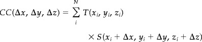
Cross correlation (CC) of target (T) and source (S) is defined for each octant by Eq. (1) [Castleman, 1996]
 |
(1) |
where (x i, y i, z i) ⊂ Octant
and N is the number of voxels in the octant. Fast‐CC is performed using Fourier transforms as follows
| (2) |
where ℑ︁ denotes Fourier transform, ℑ︁‐1 inverse Fourier transform and bar represents complex conjugate [Castleman, 1996]. The 3D displacement vector is then defined as the vector displacement (Δx, Δy, Δz) in the CC array at the point where correlation between the target and source volume is at a maximum (i.e., maximum value of CC).
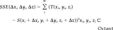
Sum square error (SSE) is defined by Eq. (3) [Christensen et al., 1993, 1995, 1996; Collins et al., 1994, 1995; Schormann and Zilles, 1998].
 |
(3) |
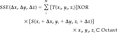
When T and S are binary values (1,0), each term in the sum of (3) yields “1” when source and target voxels are different and “0” when they are the same. Using this characteristics behavior, Eq. (3) can be simplified to an exclusive “OR” operation (XOR) as follows (see Appendix):
 |
(4) |
The 3D displacement vector is the vector with components (Δx, Δy, Δz), where SSE, tested for all possible translations, is minimal. This is the displacement with minimal dissimilarity between the source and target tissue templates.
Mismatch assessment
The progress of the registration during the OSN processing is assessed in three ways: boundary mismatch, the number of source brain octants declared as noncomparable, and the difference between target and source tissue volumes. Boundary mismatch is calculated for each template region by counting the number of mismatched voxels (source brain not matching target brain) in the transformed source brain. Because of its intrinsically high sensitivity to error, the calculated boundary mismatch was used to evaluate the matching performance of the three feature matching schemes (geometrical centroids, CC, and SSE).
The second mismatch measure is the number of source brain octants that do not initially have voxels matching the dominant feature of the target octants. This assessment is not a direct measurement of tissue mismatch but provides insight into the level of feature homology between the source and target brains.
The third assessment, total volume mismatch, uses Eq. (5) to calculate the percent difference in the total volume for each tissue type between source and target regions.
| (5) |
While total volume mismatch does not measure the quality of the regional match between source and target tissues, it is a measure of the global match between target and transformed source tissue volumes.
MATERIAL AND METHODS
Evaluation of similarity measurements procedures
OSN was tested on six MRI brain volumes randomly selected from a group of 11 volumes from a previous study [Kochunov et al., 1999], and a target brain was randomly selected from the same group. All source brains were globally spatially normalized using the Convex Hull method [Lancaster et al., 1999] prior to evaluation. Four feature matching methods were evaluated: geometrical centroids, fast‐CC, SSE, and a combination of fast‐CC and centroid. The similarity measurement performance was monitored at each step of OSN processing by determining the boundary mismatch for GM and WM template regions. The feature matching scheme with best overall matching capabilities was then used for all other testing of OSN.
Multiple iterations of OSN algorithm
Multiple iterations of the OSN algorithm improve the feature matching by continuously modifying displacement vectors in the deformation field (DF). After all seven steps of the first iteration are performed, the second iteration repeats steps 1 through 7 (2563 data) with the DF being updated at every step, and so on. The DF is continuously refined by this iterative process. The best similarity measurement routine (above) was used to evaluate multiple iterations, with the fit quality monitored by boundary mismatch. It was expected that after a certain number of iterations the fit quality would maximize with no improvement obtained with additional iterations. The number of iterations of OSN where the fit quality maximizes was determined and that number was used in subsequent processing tests.
Multiple application of OSN algorithm
The feasibility of applying OSN multiple times (runs) was evaluated. Unlike iteration, each run is performed using the transformed image of the previous run as the source volume. The DF for each run is stored in the file. When an acceptable tissue match is achieved, stored DFs are consequently applied one by one to the MR image volume using sinc or trilinear interpolation. The mismatch was monitored by boundary mismatch. Again it was expected that after several runs the fit quality would maximize with little further improvement.
Lateral ventricle mismatch
Lateral ventricle mismatch between the target and source brains was evaluated following global and OSN normalization to compare with previously published reports [Collins et al., 1994, 1995]. Two mismatch assessments were used: total volume difference and boundary mismatch. Voxels containing lateral ventricles in the target and source volumes were segmented, and the total volumes were measured and compared. To measure the boundary mismatch an XOR operation was performed between the source and target ventricle volumes. Note, that this logical operation approach is identical to that in the sum square error (SSE) similarity measurement approach given by Eq. (4). This operation results in an image with a value of 1 where the ventricle was not present in both the target and source images. Errors along the boundary of the ventricle were generally one‐voxel‐thick and were not considered as failure to match but rather as interpolation artifacts. Therefore a 3 × 3 median filter was used to eliminate these residual interpolation errors for the voxels around the boundary of the ventricle while preserving significant regions of volumetric mismatch.
Assessment of matching of major sulci
Preliminary processing
The ability of OSN to warp cortical sulci to consistent anatomical locations was tested on nine MR brain volumes of healthy volunteers. The data were provided for nonlinear warping algorithm comparison by the ICBM project [Mazziotta et al., 1995]. For each of the brain volumes, manual bilateral tracings of major cortical sulci and fissures were provided as a list of 3D coordinates. A target brain was randomly selected from the group and the remaining eight brain volumes were transformed to mach it. The brain volumes were thresholded at 25% of their mean value to dilate sulcal folds prior to template creation. A single run of OSN processing with three iterations was used to regionally match all volumes to the target. The eight brain volumes and sulcal tracings were individually transformed to the target brain volume using OSN deformation fields.
Evaluation of fit quality
The fit quality for major anatomical features (sylvian fissure, precentral sulci, central sulci and postcentral sulci) was evaluated by calculating the spatial variance of individual tracings of sulci around their mean tracing. This spread was calculated for the eight brains before and after OSN processing. To numerically quantify spatial mean and variance, the curves were parameterized using B‐splines. This parameterization of sulcal tracings provides a method to estimate coordinates at any point along sulci as a function of the parameter t, where t is defined between zero and tmax (locations of the curve's endpoints). We used freeware C++ code from http://www.magic-soft ware.com/ to create parameterized curves. The 3D curve class, provided in this code, takes a list of 3D coordinates and reconstructs smooth 3D curves (where both the first and the second derivatives are continuous) using fourth‐order B‐splines.
Four bilateral tracings in eight subjects were parameterized. The x, y, and z coordinates corresponding to the midpoint of each structure's parameterized curve were averaged across subjects to obtain an average midpoint site for each structure. For each structure's curve we determined tmid as the closest point to the midpoint site as the reference point for calculating spatial spread of the structure. The radial standard deviation of the eight subject's parameterized curves relative to the mean tracing was calculated with 1 mm steps along the mean parameterized curve.
RESULTS
Automated segmentation procedure
Figure 1 shows an axial section image from the target brain at z = 24 (Talairach coordinate) with boundaries of outer GM (red), deep GM (blue), and lateral ventricle (green) as defined in Herndon et al. [1998]. The red outline illustrates the clear separation between WM and cerebral cortex and the boundaries between deep gray and WM and the lateral ventricle. Fine structure in sulci is lost due to the 3 ×3 opening‐closing operation performed to remove nonconnected components. This operation reduces the resolution of the segmented image to the limiting resolution of OSN (2 × 2 × 2 voxels). However, a well‐defined edge that separates major tissues is seen throughout the brain.
Figure 1.
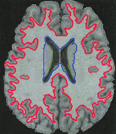
Slice at Z = 24 (Talairach coordinates) with borders of GM and WM (red), deep GM, and WM (blue), and CSF (green).
Evaluation of similarity measurements procedures
Figure 2 shows boundary mismatch at each step of the first iteration of OSN processing. The trend for the SSE and CC curves was similar but differed significantly from that of the centroid curve. The centroid method for GM and WM shows less improvement through step 4 when compared to CC and SSE methods. For GM the situation changes after step four, as the slope of the centroid curve does not change while the SSE and CC curves level off. The CC‐centroid method performed well during the first steps due to the uses of the CC criterion and during latter steps due to the switch to centroid processing. The SSE curve appears similar to the CC curve, but the SSE execution time was excessive when compared with the fast‐CC method (13 hr vs. 10 min). The combined fast‐CC/centroid method was chosen as the most appropriate method based on overall performance and processing time (total OSN execution time is only 7 min).
Figure 2.
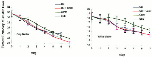
Gray and white matter boundary mismatch with every step of the first iteration of OSN processing for four tested methods: CC (blue), CC + centroid (red), centroid (green), SSE (cyan).
Multiple iteration
A multiple iteration approach was evaluated using the fast‐CC/centroid matching method. The boundary match improved as the number of iterations increased. A significant improvement was seen in the second iteration for both GM and WM regions of the brain template (Table I). In the third iteration, little improvement is seen. This result suggests that two iterations of the OSN algorithm are adequate for matching critical tissues.
Table I.
Percent tissue boundary mismatch improvement by iteration
| Iteration | GM | WM |
|---|---|---|
| 2 vs. 1 | 14.5 ± 5.4% | 9.8 ± 3.0% |
| 3 vs. 2 | −0.8 ± 1.3% | 1.7 ± 2.0% |
n = 5 subjects
Multiple applications of the OSN algorithm
The results of multiple runs of the OSN algorithm are shown in Table II where total tissue volumetric mismatch is shown after applying the OSN algorithm for one, two and three runs. Two iterations were used in each run using the fast‐CC/centroid similarity measurement method.
Table II.
Total boundary mismatch by run
| Run | GM | WM |
|---|---|---|
| Global | 31.6 ± 5% | 19 ± 5.4% |
| Run 1 | 17.5 ± 3.0% | 13.2 ± 2.3% |
| Run 2 | 12.8 ± 2.5% | 11.7 ± 1.8% |
| Run 3 | 9.5 ± 2.3% | 11.2 ± 1.6% |
n = 5 subjects
The most significant improvement was observed for run 1. Improvement for runs 2 and 3 are less substantial (Table II). The standard deviation decreased with each run. Table III shows the absolute volume differences for global spatial normalization for runs 1–3 of the OSN algorithm. The results show that the OSN algorithm significantly reduced the absolute volume difference.
Table III.
GM and WM volume difference between target and OSN transformed brains
| Run | GM | WM |
|---|---|---|
| Global | 8.0 ± 2.1% | 4.2 ± 1.3% |
| Run 3 | 2.5 ± 0.5% | 2.9 ± 0.9% |
n = 5 subjects
Figure 3 shows that the estimated percent of noncomparable octants for each octant size in the source volume gradually decreased with successive runs of OSN. The greatest decrease was observed for the first and second runs. Little improvement was seen for run 3. The estimated number of noncomparable octants was decreased by a factor of six after three runs of the OSN processing.
Figure 3.
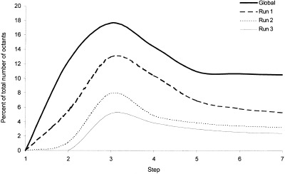
Percent of noncomparable octants encountered for every step of three runs of OSN.
Figure 4 illustrates regional transformation capabilities of OSN when applied to a gray‐scale image. A deformation field, obtained from two runs of OSN with two iterations each, was applied to the source gray‐scale data using trilinear interpolation. Gross failures of global spatial normalization are illustrated for sagittal, axial, and coronal sections by arrows (Fig. 4, top). A significant improvement in regional spatial matching afforded by OSN is illustrated in the paired section images, Figure 4 (bottom). The white matter contours (red outline) also reveal only small residual GM/WM mismatch following the regional warping.
Figure 4.
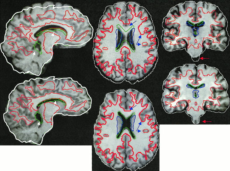
Sagital, axial, and coronal views of a brain before (top) and after (bottom) OSN processing. The arrows show areas of significant improvement.
Lateral ventricle mismatch
Table IV shows the average percent volumetric difference of the lateral ventricle following global SN and 1 and 3 runs of OSN normalization, which corresponds to 15 and 50 min of processing time. Both absolute difference and standard deviation were significantly reduced.
Table IV.
Lateral ventricle volume difference and boundary mismatch by run
| Run | Volume difference | Boundary mismatch |
|---|---|---|
| Global | 60 ± 20% | 55.0 ± 10.0% |
| Run 1 | 20 ± 3% | 22.1 ± 3.0% |
| Run 3 | 5.2 ± 1.5% | 7.1 ± 1.0% |
n = 5 subjects
Table IV shows percentage boundary mismatch following global, OSN run 1, and OSN run 3 normalization steps. Again, both the boundary mismatch and its standard deviation were significantly reduced.
Assessment of matching of major sulci
Figure 5 shows the high degree of residual anatomical variability of the four bilateral sulcal structures in eight brains following global spatial normalization (top row) and the reduction in residual anatomical variability following OSN processing (bottom row).
Figure 5.
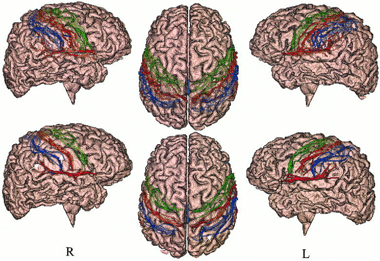
Right (R), top, and left (L) views of sulcal tracings from eight subjects following global spatial normalization (top) and OSN processing (bottom) overlaid on the target brain. White arrows highlight several areas of anatomically poor match.
The radial standard deviation of individual tracings around the mean sulcal curve is shown for all four structures in Figure 6 as a quantitative index of anatomical variability. The discontinuities observed at the ends of the graphs were due to differences in length of individual tracings. The graphs show a reduction of anatomical variability for every cortical tracing following OSN processing. These patterns are consistent with sulci variability illustrated graphically in Figure 6. The spatial variability of the central sulcus following global spatial normalization was higher in the right hemisphere than in the left hemisphere, which is consistent with Ziles et al. [1997]. The most significant reduction was observed in the right central sulcus and left precentral sulcus. Both of these anatomical structures were well isolated from other cortical folds, which made it easier for OSN to track corresponding anatomical features. The least reduction in anatomical variability was observed in the right postcentral sulcus. The residual high variability in that region was due to incorrect anatomical feature pairing in 3 out of 8 right postcentral sulci (Fig. 5, white arrows): two were paired with the parietal‐occipital sulcus of the target, and the third was paired with the target's central sulcus. This failure of feature pairing was attributed to the unusual anatomy of the target (central and parietal occipital sulci are cramped closer on the right than on the left) and high spatial variability of right postcentral sulci following global spatial normalization [Talairach et al., 1988; Thompson et al., 1996, 2000].
Figure 6.
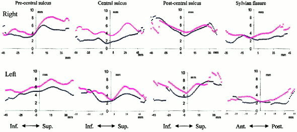
Spatial variance of sulcal tracings plotted along the length of the sulcal tracings (zero point indicates the middle of the tracing) before (x) and after (o) OSN processing.
The mean OSN transformed sulcal tracings and target brain sulcal tracings are overlaid on the target brain surface in Figure 7. This figure demonstrates the accuracy of OSN method showing little transformation bias along any of the four sulci.
Figure 7.
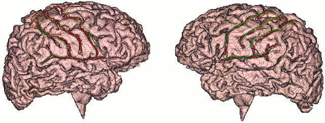
Mean intersubject (green) and target (red) sulcal tracing overlaid on the target's brain surface.
DISCUSSION
Template warping
While one of the reported uses of regional spatial normalization is to perform anatomical segmentation and labeling, Collins and coworkers [1995], acknowledged unsatisfactory performance of the ANIMAL algorithm in matching cortical structures. They also showed that when the anatomical information was more explicit, such as automatically labeled major cortical sulci, the fit was significantly improved. While gray‐scale images contain this information, the extraction and analysis within the warping loop is time prohibitive. The approach to resolve this problem proposed by Collins et al. [1999] was to develop a sidetrack of applications to perform anatomical segmentation and anatomical feature extraction to assist in gray‐scale warping. In the modified OSN presented here, we eliminated gray‐scale warping by creating anatomical templates that represent, but that are not limited to, a collection of anatomical features. The deformation field that is obtained is then used to warp anatomical and/or functional data. Plans to add functional templates are under consideration.
The main argument against this kind of processing is that current segmentation procedures are not sufficiently robust to perform reliable segmentation. While this is true for matching down to single voxels, the automated segmentation routines currently developed perform segmentation of major structures on a par with human observers [Xu et al., 1999; Dastidar et al., 2000]. In fact, even well‐trained humans cannot reliably segment down to the limiting resolution of MRI, partly due to limited SNR and partly due to partial volume averaging artifacts. Thus, any gray‐scale volumetric warping algorithm is susceptible to the same problems and MR artifacts. The use of anatomical templates supports incorporation of newer and more robust segmentation algorithms in a facile way. Also, additional features such as automatically extracted major sulci and even functional data can be included without modification of the warping algorithm.
Automated segmentation procedure
The segmentation procedure of Herndon et al. [1998] was shown to provide fast and reliable definitions of tissue borders with a resolution limited only by the resolution of the MR image. A requirement for this routine is that an operator provide values for WM, GM, and CSF for each individual image volume. This method works well to adapt individual images to a standard segmentation scheme. While there are known limitations to any segmentation process, this method was considered adequate for testing and evaluation during the development of OSN. With minor modification, the OSN algorithm can be used with any brain segmentation routine that produces segmented output (GM, WM, CSF). Brain tissue segmentation is a rapidly developing area of brain image processing with new methods being published on a regular basis [Scholesinger et al., 1997; Xu et al., 1999]. Also, progress in MR imaging should provide better tissue contrast and SNR, which allows for more accurate segmentation at the limiting MR resolution with the current segmentation methods.
Evaluation of similarity measurements procedures
The CC and SSE methods had similar trends, i.e., continual improvement in boundary mismatch during the first steps (1–4) with less improvement in subsequent steps (5–7) (Fig. 2). Both of these similarity measurement methods calculate deformation components that optimize the overlap between target and source template features. This strategy should work well if compared features are similar in shape and size (i.e., geometrically homologous). This is believed to partly account for the good performance of the CC and SSE methods during steps 1–4, which deal with larger structures that are expected to be more geometrically similar. Conversely, the third similarity measurement method, based on centroids, is not sensitive to either size or shape, and it did not perform as well for steps 1–4.
It is believed that as smaller octants are analyzed (steps 5–7) the geometrical similarity of the dominant features begins to fail, and this partly accounts for the poor performance of the CC and SSE methods in that range. It is not clear why the centroid method continued to show improvement for steps 5–7. However, results indicate that when geometrical homology becomes a problem, the centroid method continues to provide meaningful deformations, i.e., to improve boundary matching. Interestingly, switching from the CC method to the centroid method after step 4 performed better than either method did individually. The switch to the centroid method at step 5 was done where the octant dimension fell just below 1 cm (0.8 cm). This observation will be studied more carefully as we continue to develop and optimize the OSN processing algorithm.
Multiple iteration
The boundary mismatch (Table III) was significantly improved after two iterations, but very little improvement was seen for the third iteration. OSN fitting progress appears to reach an equilibrium due to continuity constraints imposed by the continuity correction method. The tight constraints on the allowable voxel shifts relative to neighboring voxels limits the amount of deformation that can be stored in a DF. Current continuity control limits local displacement of each voxel (relative to its neighbors) to 0.3 of a voxel dimension in x, y, and z directions, which ensures that discontinuity is avoided [Kochunov et al., 1999]. In some instances it is overly conservative, especially if a local deformation consists of a single component only (e.g., deformation with a vector [0.5,0,0] will be considered as a threat to the continuity, even though this is not the case and will be replaced by a vector [0.3,0,0] following the continuity correction). Continuity assessment and modulation using the Jacobian [Kochunov et al., 1999] will be evaluated in the future. This could possibly reduce the number of iterations and/or runs needed to achieve the current fit quality.
Multiple applications of the OSN algorithm
Applying OSN multiple times is the current solution to overcome restrictions imposed by continuity correction on the amount of deformation that can be stored in a deformation field (as discussed in the previous section). The boundary mismatch reduces significantly after running OSN two times and levels off after the third run. When acceptable tissue match is achieved, the stored DFs are applied one by one to the MR image volume using sinc or trilinear interpolation. An example of this processing is demonstrated in Figure 4. Two runs of OSN with two iterations were used to warp anatomical templates. The resulting DFs were consequently applied to the original data using trilinear interpolation. The overlaid target's outlines show significant improvement following OSN normalization. This improvement can be seen for the lateral and third ventricle in the sagital view (Fig. 4, white arrows). The blue arrows (axial view) depict an improvement in gray vs. white matter matching. The red arrows (coronal view) depict an improvement in the brain stem match. The total processing time including interpolation was less then 30 min on a Sun Ultra 30, 250 MHz workstation (Sun, Mountain View, CA).
The major disadvantage of this approach lies in the interpolation routine. The trilinear interpolation routine, used in this processing is fast (2 min to transform a 2563 brain image) but introduces spatial smoothing (Fig. 4, bottom vs. top) with each application and thus reduces the spatial resolution of the final image. A sinc interpolation routine preserves the original resolution of a MR image [Hajnal et al., 1995] but it is much slower than trilinear interpolation. In fact, it currently takes about 30 min to perform a sinc‐interpolation‐based transformation. We are investigating an approach to concatenate separate DFs to support using a single interpolation for reconstruction. This will permit using a single transformation with the trilinear interpolation because smoothing artifacts from a single application of trilinear interpolation are minor with isometric high‐resolution MR images, and overall processing time for interpolation can be reduced to 1 min.
Lateral ventricle mismatch
The evaluation of the lateral ventricles shows that OSN can perform extremely well while matching even down to small boundary details. The boundary mismatch and absolute volume differences were reduced to less then 10% of the target ventricle volume, which is consistent with previously reported values [Collins et al., 1995]. The number of runs needed to achieve the low percentage boundary mismatch will hopefully be reduced to one by optimizing regional modulation of continuity correction. Additionally we plan on implementing a regional control of the shift from CC to centroid matching based on measured correlation, which may allow us to reach current level of fit throughout the brain with one iteration and one run.
Assessment of matching of major sulci
OSN processing was shown to significantly decrease the volumetric template tissue mismatch. While volumetric mismatch is a potent mismatch assessment, it does not measure anatomical correctness. Assessment of sulcal warping provides a measure of anatomical fit quality that is familiar for atlas based comparisons. Most of the studies reporting volumetric algorithms did not investigate sulcal match [Bajcsy and Broit, 1982; Bajcsy and Kovacic, 1989; Miller et al., 1993; Christensen, 1999; Christensen et al., 1994, 1996; Collins et al., 1994, 1995]. To date there has been only one publication that illustrated sulcal warping performance of a volumetric regional spatial normalization algorithm [Collins et al., 1999]. In that study, the sulci information was explicitly used to drive the transformation algorithm and major sulci were manually traced in transformed images. In the OSN study sulcal information was not explicit in the template. The sulci were manually traced prior to OSN processing and then transformed from source to target brains using derived deformation fields. While OSN warps an entire volume it does not match sulci explicitly (e.g., central to central); rather, the warp is based on the correspondence between local TDF features of source and target templates. Examples of residual anatomical mismatch in major sulci are seen in Figure 5 (white arrows). In these cases, failed sulcal correspondence following automated global spatial normalization (CHSN) [Lancaster et al., 1999] created a false sulcal features correspondence (e.g., source brain postcentral sulcus was overlaid on the target's parietal‐occipital sulcus), which could not be resolved by OSN. The sulcal mismatch problems can be avoided if more complete anatomical information are included in the brain template (e.g., each sulcal region in the template explicitly identified). Collins et al. [1999] tested this idea and showed that the ANIMAL algorithm driven by gray‐scale data alone performs on par with global spatial normalization for matching cortical sulci. Using sulcal information improved the sulcal fit significantly. In Collins's study the sulci were automatically identified with a new processing method called SEAL (Sulcal Extraction and Automated Labeling) [Le Goualher et al., 1996, 1997]. Although the OSN template did not include labeled sulci, Figures 5, 6, 7 show that OSN processing significantly improved sulcal fit, which suggests an inherit superiority of the basic algorithm over the ANIMAL approach. We are currently exploring the incorporation of a more accurate anatomical segmentation methods such as SEAL [Le Goualher et al., 1996, 1997] to provide an even greater match in the sulci throughout the brain.
The choice of the target is also an import issue since matching a target brain anatomy that differs greatly from the norm will produce more errors than matching to a target closer to the norm. A possible solution is to construct an anatomical template that represents an average anatomy of the group by averaging individual brain volumes in the standardized space [Thompson et al., 2000].
CONCLUSION
The octree spatial normalization (OSN) method was found to be fast with accuracy comparable to or better then existing methods. Anatomical template warping was selected as opposed to gray‐scale warping used in the previously published method [Kochunov et al., 1999]. An automated tissue segmentation procedure was adapted to create anatomical templates by classifying a brain image into WM, GM, and CSF. The best match quality and processing efficiency were found by combining fast cross‐correlation in larger octants with centroid feature matching in smaller octants. The need to switch the feature matching strategy is believed to be the result of loss of feature homology in smaller octants.
Two runs with two iterations of OSN were found to be sufficient to match images well while keeping processing time at half an hour on a Sun Ultra‐30, 250MHz (Sun, Mountain View, CA). Mismatch for GM, WM, and lateral ventricles in a group of six subjects showed a significant reduction of both boundary mismatch and absolute volume differences.
OSN reduced anatomical variability for the each of the evaluated sulci, and intersubject mean tracings were found to correspond well with target tracings. A need to incorporate anatomical information into the templates was observed, and we are currently investigating automated sulcal and cortex extraction methods [Le Goualher et al., 1996, 1997; Xu et al., 1999] for this purpose.
APPENDIX I.
The argument of the summation in Eq. (3) can be rewritten as T 2 − 2 · S · T + S 2. This equation has the same truth table as T XOR S as shown in Table 1 when T and S are binary. Thus it can be replaced with T XOR S operation for efficiency purposes.
| T | S | T XOR S | T 2 − 2 · S · T + S 2 |
|---|---|---|---|
| 0 | 0 | 0 | 0 |
| 0 | 1 | 1 | 1 |
| 1 | 0 | 1 | 1 |
| 1 | 1 | 0 | 0 |
Table 1. The truth table for exclusive OR operation.
Edited by: Karl Friston, Associate Editor
REFERENCES
- Ashburner J, Friston KJ (1999): Nonlinear spatial normalization using basis functions. Hum Brain Mapp 7: 254–266. [DOI] [PMC free article] [PubMed] [Google Scholar]
- Bajcsy R, Broit C (1982): Matching of deformed images. In: IEEE Proceedings of the 6th international conference on pattern recognition. Munich, Germany: p 351–353.
- Bajcsy R, Kovacic S (1989): Multiresolution elastic matching. Computer Vision Graphics Image Process 46: 1–21. [Google Scholar]
- Castleman K (1996): Digital image processing. Englewood: Prentice Hall, p 115–141. [Google Scholar]
- Christensen G, Rabbitt R, Miller M (1994): 3D brain mapping using a deformable neuroanatomy. Physics in Med and Biol 39: 609–618. [DOI] [PubMed] [Google Scholar]
- Christensen G, Rabbitt R, Miller M, Joshi S, Grenander U, Coogan T, Van Essen D (1995): Topological properties of smooth anatomic maps In: Bizais Y, Braillot C, Di Paola R, editors. Information processing in medical imaging: 14th international conference. Boston: Kluwer, p 101–112. [Google Scholar]
- Christensen G, Rabbitt R, Miller M (1996): Deformable templates using large deformattion kinematics. IEEE Trans Image Processing 5: 1435–1437. [DOI] [PubMed] [Google Scholar]
- Christensen G (1999): Bayesian framework for image registration using eigenfunctions In: Toga AW, editor. Brain warping, Academic Press, p 85–100. [Google Scholar]
- Collins D, Neelin P, Peters Y, Evans A (1994): Automatic 3D intersubject registration of MR volumetric data in standardized space. J Comput Assist Tomogr 18: 192–205. [PubMed] [Google Scholar]
- Collins D, Holmes C, Peters T, Evans A (1995): Automatic 3D model‐based neuroanatomical segmentation. Hum Brain Mapp 3: 190–208. [Google Scholar]
- Collins D, Holmes C, Peters T, Evans A (1999): ANIMAL: Automated nonlinear image matching and anatomical labeling In: Toga AW, editor. Brain warping. San Diego: Academic Press, p 133–142. [Google Scholar]
- Dastidar P, Heinonen T, Ahonen JP, Jehkonen M, Molnar G (2000): Volumetric measurements of right cerebral hemisphere infarction: use of a semiautomatic MRI segmentation technique. Comput Biol Med 30: 41–54. [DOI] [PubMed] [Google Scholar]
- Downs H, Lancaster J, Fox P (1998): Surface‐based spatial nomalization using convex hull In: Toga AW, editor. Brain warping. San Diego: Academic Press, p 263–281. [Google Scholar]
- Foley J, van Dam A, Feiner S, Hughes J (1990): Computer graphics principles and practice, 2nd ed. Reading: Addison‐Wesley, Chapter 6 Addison‐Wesley. [Google Scholar]
- Fox P, Perlmutter J, Raichle M (1985): A stereotactic method of anatomical localization for positron emission tomography. J Comput Assist Tomogr 9: 141–153. [DOI] [PubMed] [Google Scholar]
- Fox P, Lancaster J (1994): Neuroscience on the net. Science 266: 1793. [DOI] [PubMed] [Google Scholar]
- Fox P (1995): Spatial normalization origins: objectives, applications, and alternatives. Hum Brain Mapp 3: 161–164. [Google Scholar]
- Fox P, Lancaster J, Parsons L, Xiong J, Zamarripa F (1997): Functional volume modeling: theory and preliminary assessment. Hum Brain Mapp 5: 306–311. [DOI] [PubMed] [Google Scholar]
- Friston KJ, Ashburner J, Frith CD, Poline JB, Heather JD, Frakowiak RSJ (1995): Spatial registration and normalization of images. Hum Brain Mapp 3: 165–189. [Google Scholar]
- Hajnal J, Saeed N, Soar E, Oatridge A, Young I, Bydder G (1995): A registration and interpolation procedure for subvoxel matching of serially acquired MR images. J Comput Assist Tomogr 19: 289–296. [DOI] [PubMed] [Google Scholar]
- Herndon C, Lancaster J, Toga A, Fox P (1996): Quantification of white matter and gray matter volumes from T1 parametric images using fuzzy classifiers. J Magn Reson Imaging 6: 425–435. [DOI] [PubMed] [Google Scholar]
- Herndon C, Lancaster J, Giedd J, Fox P (1998): Quantification of white matter and gray matter volumes from three dimensional magnetic resonance volume studies using fuzzy classifiers. ISMRM 8: 1097–1105. [DOI] [PubMed] [Google Scholar]
- Kochunov P, Lancaster J, Fox P (1999): Accurate high‐speed spatial normalization using an octree method. NeuroImage 10: 724–737. [DOI] [PubMed] [Google Scholar]
- Lancaster JL, Glass TG, Lankipalli BR, Downs H, Mayberg H, Fox PT (1995): A modality‐independent approach to spatial normalization of tomographic images of the human brain. Hum Brain Mapp 3: 209–223. [Google Scholar]
- Lancaster JL, Rainey LHTG, Summerlin JL, Freitas CS, Fox PT, Evans AC, Toga AW, Mazziotta JC (1997): Automated labeling of the human brain: a preliminary report on the development and evaluation of a forward‐transform method. Hum Brain Mapp 5: 238–242. [DOI] [PMC free article] [PubMed] [Google Scholar]
- Lancaster JL, Kochunov PV, Fox PT, Nickerson D (1998): k‐tree method for high‐speed spatial normalization. Hum Brain Mapp 6: 358–363. [DOI] [PMC free article] [PubMed] [Google Scholar]
- Lancaster J, Fox P, Downs H, Nickerson D, Hander T, Mallah M, Zamarripa F (1999): Global spatial normalization of the human brain using convex hulls. J Nucl Med 40: 942–955. [PubMed] [Google Scholar]
- Mazziotta JC, Toga AW, Evans A, Fox P, Lancaster J (1995): A probabilistic atlas of the human brain: theory and rationale for its development. NeuroImage 2: 89–101. [DOI] [PubMed] [Google Scholar]
- Miller M, Christensen G, Amit Y, Grenander U (1993): Mathematical textbook of deformable neuroanatomies. Proc Natl Acad Sci 90: 11944–11948. [DOI] [PMC free article] [PubMed] [Google Scholar]
- Roland PE, Graufelds CJ, Wahlin J, Ingleman L, Andersson M, Ledberg A, Pederson J, Akerman S, Dabringhaus A, Zilles K (1994): Human brain atlas: for high‐resolution functional and anatomical mapping. Hum Brain Mapp 1: 127–184. [DOI] [PubMed] [Google Scholar]
- Studholme C, Hill D, Hawkes D (1995): Multiresolution voxel similarity measurments for MR‐PET coregistration In: Bizas Y, Barillot C, DiPaula R, editors. Information processing in medical imaging. Dordrecht: Klower Academic Publishers, p 287–298. [Google Scholar]
- Scholesinger DJ, Snell JW, Mansfield LE, Brookeman JR, Downs JH, Ortega JM, Kassell NF (1997): Segmentation of cortical surface and interior brain structure using active surface/active volume templates. SPIE Medical Imaging Proceedings.
- Schormann T, Zilles K (1998): Three‐dimensional linear and nonlinear transformations: an integration of light microscopical and MRI data. Hum Brain Mapp 6: 339–347. [DOI] [PMC free article] [PubMed] [Google Scholar]
- Talairach J, Tournoux P (1988): Co‐planar stereotaxic atlas of the human brain. New York: Thieme Medical Publishers. [Google Scholar]
- Thompson P, Schwarts C, Lin R, Khan A, Toga A (1996): Three dimensional statistical analysis of sulcal variability in the human brain. J Neurosci 16: 4261–4274. [DOI] [PMC free article] [PubMed] [Google Scholar]
- Thompson P, Woods R, Mega M, Toga A (2000): Mathematical/computational challenges in creating deformable and probabilistic atlases of the human brain. Hum Brain Mapp 9: 81–92. [DOI] [PMC free article] [PubMed] [Google Scholar]
- Toga A, Thompson P (1999): An introduction to brain warping In: Toga AW, editor. Brain warping. San Diego: Academic Press, p 1–26. [Google Scholar]
- Woods R (1996): Correlation of brain structure and function In: Toga A, Mazziotta J, editors. Brain mapping the methods. San Diego: Academic Press, p 313–342. [Google Scholar]
- Woods RP, Grafton ST, Watson JD, Sicotte NL, Mazziotta JC (1998): Automated image registration: II. Intersubject validation of linear and nonlinear models. J Comput Assist Tomogr 22: 153–165. [DOI] [PubMed] [Google Scholar]
- Xu C, Pham DL, Rettmann ME, Yu DN, Prince JL (1999): Reconstruction of the human cerebral cortex from magnetic resonance images. IEEE Trans Med Imaging 18: 467–480. [DOI] [PubMed] [Google Scholar]
- Zilles K, Schleicher A, Langemann C, Amunts K, Morosan P, Palomero‐Gallagher N, Schormann T, Mohlberg H, Burgel U, Steinmetz H, Schlaug G, Roland P (1997): Quantitative analysis of sulci in the human cerebral cortex: development, regional heterogeneity, gender difference, asymmetry, intersubject variability, and cortical architecture. Hum Brain Mapp 5: 218–221. [DOI] [PubMed] [Google Scholar]