A system for the generation of curves on 3D brain images

Abstract

In this study, a computational optimal system for the generation of curves on triangulated surfaces representing 3D brains is described. The algorithm is based on optimally computing geodesics on the triangulated surfaces following Kimmel and Sethian ([1998]: Proc Natl Acad Sci 95:15). The system can be used to compute geodesic curves for accurate distance measurements as well as to detect sulci and gyri. These curves are defined based on local surface curvatures that are computed following a novel approach presented in this study. The corresponding software is available to the research community. Hum. Brain Mapping 14:1–15, 2001. © 2001 Wiley‐Liss, Inc.

INTRODUCTION

The need to work with three dimensional (3D) representations of the brain has been demonstrated in many areas of computational neuroscience [Grenander and Miller, 1998; Thompson et al., 2000; Van Essen et al., 1998]. Applications that use this representation include brain flattening for visualization [Angenent et al., 1998; Wandell et al., in press; 1996; Zigelman et al., 2000], brain warping [Toga, 1998], activity detection with anatomical constraints [Faugeras et al., 1999; Kiebel and Friston, 2000], and signal detection [Sapiro, 2001]. In these applications, geometric computations are done on the surface. For example, many of the techniques for brain flattening require accurate computations of geodesic distances (that is, minimal distances while the traveling path is restricted to the surface). Sulci extraction are needed in order, for example, to impose boundary conditions to common brain warping algorithms. Segmentation of information defined on the 3D brain is needed in cases like signal detection in fMRI. In this study, we describe a system to computationally optimally (computations of the order of the minimal theoretical bound) generate weighted paths on triangulated surfaces. This system is available for the research community at http://www.ece.umn.edu/users/guille. Particular examples include geodesic distances, sulci and gyri extremes, and segmentation by tracing. We limit ourselves in this study to work with triangulated representations of the brain, being this is one of the most commonly found representations in the computational neuroscience literature. Such triangulated representations can be obtained with segmentation algorithms as those described in [Caselles et al., 1997; Joshi et al., 1999; Teo et al., 1997; Yezzi et al., 1997]. The work can easily be extended to more general polygonal representations. To extend the work here presented to implicit representations, we could use the techniques introduced in [Bertalmio et al., 1999; Cheng et al., 2000; Memoli and Sapiro, 2000]. Since many of the current state‐of‐the‐art brain segmentation algorithms obtain an implicit representation, which is later triangulated, the extension of the work here reported to these implicit surfaces is of extreme significance and will be reported elsewhere.

The basic idea of our system is to first use the technique introduced in Kimmel and Sethian [1998] for the fast computation of accurate weighted distances on triangulated surfaces. This is combined then with the work in [Cohen and Kimmel, 1997; Khaneja et al., 1998; Kimmel, 1999; Kimmel and Sethian, 1998] and new developments here presented for computing the corresponding path that achieves the minimal weighted distance (geodesic curve), the specific weight being dictated by the application (uniform for intrinsic geodesics, surface curvature dependent for sulci and gyri, and data dependent for segmentation). The novelty in this study compared with the work of Kimmel and Sethian [1998] is concentrated on the specific applications and computations of the corresponding weights and on slight modifications to the original fast computation.

Optimal weighted distances on triangulated surfaces

Curves such as sulci and gyri can be considered as shortest weighted paths on the 3D surface representation of the brain. That is, given a specific weight dictated by the application, these curves are paths of minimal total ‘effort’. These paths are geodesics on the surface (see Appendix A for a basic overview of 3D differential geometry). Given the weight then, the problem reduces to that of computation of geodesics on a surface (we will later deal with how to compute the weights for specific examples like sulci and gyri). Following Kimmel and Sethian [1998] (see also Barth and Sethian [1998] and Lafon and Osher [1996] for related works on triangulated surfaces), we present the technique used by our system to compute the weighted distance between two points x ₁ and x ₂ on the triangulated surface S _▵ that approximates the regular surface S. That is, given a seed point x ₁ ∈ S _▵, for every second point x ₂ ∈ S _▵, we want to compute the distance d ${}_{\mathit{\text{g}}\text{(}\mathit{\text{S}}{}_{\text{▵)}}}$ (x ₁,x ₂), where g(S _▵) is a given weight defined on the triangulated surface S _▵. The weighted distance between two points on the continuous surface S is given by

(1)

where ds stands for the Euclidean arc‐length (note that for g(s) = 1 we obtain, ∫${}_{\mathit{\text{x}}{}_{\text{1}}}^{\mathit{\text{x}}{}_{\text{2}}}$ ds, which is just the Euclidean distance; see also Appendix A). All the measurements are of course to be made intrinsically to the surface. That is, ds is measured on the surface S and the path that achieves the minimal distance will lay on the surface as well. If S _▵ approximates S, we are then looking for an efficient computation of d ${}_{\mathit{\text{g}}\text{(}\mathit{\text{S}}{}_{\text{▵)}}}$(x ₁, x ₂), an approximation of the true weighted distance d _g(S)(x ₁, x ₂), where x ₁, x ₂ are two arbitrary points on the surface (not necessarily the vertices in S _▵). Kimmel and Sethian [1998] have devised a computationally optimal algorithm for doing exactly this, which we briefly describe below. Note that in this section we are just discussing the computation of the distance, not the exact path (geodesic curve) that achieves the minimum. This will be addressed in the following section.

Computing minimal weighted distances and paths in graphs is an old problem that has been optimally solved by Dijkstra [1959]. Dijkstra showed an algorithm for computing the path in O(n log n) operations, where n is the number of nodes in the graph. The weights are given on the connecting edges between the graph nodes, and the algorithm is computationally optimal. Previously we described Dijkstra's algorithm using nodes in a graph. In the case of a triangulation, if we consider the vertices as nodes and edges as the connections between them, we can apply the same algorithm to compute the distances. The problem is that this algorithm is limited to travel on the graph edges, giving only a first approximation of the true distance. Let's illustrate this problem with a simple example. Assume we have a planar graph with three nodes located at the coordinates (0,1), (1,0), and (0,0); see Figure 1. Assume that we have only two edges, one from (1,0) to (0,0) and an additional edge from (0,1) to (0,0). Assume also that both edges have weight equal to one. If we use Dijkstra algorithm, we will get that the distance between (1,0) and (0,1) is 2. But we know that the distance is , and this is a very significant error. The problem here was that we were forced to travel only through the existent edges, and there is no edge between (1,0) and (0,1). The same problem happens in more elaborated graphs, including triangulated surfaces (the path from a vertex to the middle of the opposite side on a given triangle will be wrongly computed for example). One algorithmic way of solving this problem is to add nodes and edges, or to heuristically add weights to the edges. This will both increase the complexity of the algorithm and will actually not converge to the true continuous weighted Euclidean distance when the resolution goes to infinity (in other words, d ${}_{\mathit{\text{g}}\text{(}\mathit{\text{S}}{}_{\text{▵)}}}$(x ₁, x ₂) will not converge to d _g(S)(x ₁, x ₂)). That is, Dijkstra is not a consistent algorithm [Mitchell, 1988; Mitchell et al., 1987]. Moreover, because Dijkstra is limited to travel graph edges, multiple minimal paths can appear. This is eliminated with the increased accuracy provided by the algorithm discussed here.

Figure 1.

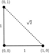
Dijkstra's distance approximation is restricted to travel on graph edges. In this simple example we will get that distance from (1, 0) to (0, 1) is 2, but we know that it is .

The solution to this problem with Dijkstra, limited to Cartesian grids, was developed in Helmsen et al. [1996], Sethian [1996a,b], Tsitsiklis [1995], and recently extended in Osher and Fedkiw [2000]. Tsitsiklis [1995] first described an optimal‐control type of approach, whereas independently Sethian [1996b] and Helmsen et al. [1996] developed techniques based on upwind numerical schemes (see below). The solution presented by these authors is consistent and converges to the true distance [Rouy and Tourin, 1992; Tsitsiklis, 1995], while keeping the same optimal complexity of O(n log n). This work was later extended in Kimmel and Sethian [1998] for triangulated surfaces, which we describe below.

The basic idea behind the optimal techniques for finding accurate weighted distances is to note that the distance function holds the following Hamilton‐Jacobi partial differential equation (PDE), e.g., Bruckstein [1988], Kimmel [1999], Osher [1993], Osher and Sethian [1988], and Sethian [1996b]:

(2)

where d is the distance from a given seed point to the rest of the space (recall that g is known, it is the given weight). Intuitively, the smaller the weight g, the larger the intrinsic distance we can travel without significantly changing the weighted distance d, making its gradient small. So we can transform the problem of optimal distance computation into the problem of solving a Hamilton‐Jacobi PDE. We now describe an O(n log n) technique for solving this PDE.

Solving the Hamilton‐Jacobi |▿d| = g on a triangulated surface

The main idea to obtain a computationally efficient solution to equation (2), the so‐called Eikonal equation, rests on building the solution outwards from lower distance values to higher ones, marching the solution in an upwind direction. This is simply imitating the Dijkstra technique for minimal paths on graphs. Initially we specify a seed set (in our case this is just a point, x ₁), that will have zero distance value. The distance function is then computed in a growing fashion, starting from the seed point, and progressively computing the distances for closest points first. The procedure stops when the whole domain has been covered.

The first part of the global distance computation is then how to locally propagate the distance inside a given triangle, when some of the vertices of this triangle have already been assigned a distance and some not. Consider the triangle ABC, as shown in Figure 2. Here we want to update the distance value at vertex C. The idea is to fit a plane over the triangle, given the distance values at the other two vertices d(A) and d(B), and the slope g (corresponding to the right hand side of the Eikonal equation). Details on how this plane fitting, and therefore the propagation, is done are given in Appendix B.

Figure 2.

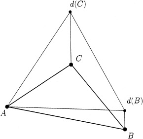
Update procedure for triangle ABC. We want to compute the distance value at C, fitting a plane over the triangle, based on A and B distances, and the desired plane slope g. For simplicity, we assume d(A) = 0.

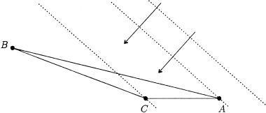
For monotonicity reasons we require the triangulation to be acute. This is so that any front (growing boundary in the distance construction method) entering the side of a triangle has two points to provide values before the third one is computed. This way we restrict the update to come from within the triangle. To see this, consider the situation in Figure 3, where we have considered an obtuse triangle ABC, and the arrows show the direction of the advancing front. In this case, the front would first reach point A, then point C, and finally point B. So, point C is supported only by point A, which means that the actual direction of the coming front can not be recovered.

Figure 3.

Obtuse triangles in distance computations. Arrows show the growing direction of the distance (i.e., it's negative gradient direction). The front would first reach point A, then C, and finally B. Therefore, C is only supported by A so we can not recover the actual direction of the front. As we restrict the update to come from within the triangle (that is, the gradient direction must lay within the angle

, a situation like this can only occur if

is obtuse.

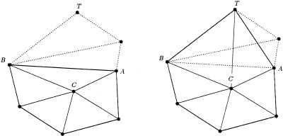
Non‐acute triangles thus require a special treatment in which every obtuse angle is split up into two acute ones. To do this we introduce a fourth vertex, T ∈ S _▵, so we now have two triangles: ATC and BTC (see Fig. 4). The procedure to find T involves its search in the unfolded adjacent triangles (this means that triangles in the surface are recursively unfolded into a plane), where the search is restricted to a limited section of incoming fronts (shaded region in Fig. 4 [right]). This limited section, obtained between the perpendiculars to both sides of the obtuse angle, guarantees that each resulting triangle would be acute, as required. Once we have the two new triangles, we apply the usual update procedure (described in Appendix B) to each of them.

Figure 4.

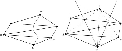
Handling procedure for obtuse triangles. Triangle ABC is divided into two acute triangles, ATC and BTC. Left: Triangulated surface in 3D space. Right: Unfolded surface in the plane. The shaded region shows the limited section of incoming fronts for vertex C.

The construction procedure described above introduces a new neighboring relation between vertex C (where the obtuse angle occurs) and vertex T. As we will see, this causes the need of special handling procedures (and slight modifications to the original algorithm) in both constructing the distance function and obtaining the exact geodesic path from the back propagating algorithm described in the following section. These special procedures are only needed when we have non‐uniform weights (i.e., g is not constant), as in our case.

The nature of the upwind operators used by the algorithm guarantee that the solution is build in a monotonous fashion, i.e., from lower distance values to higher ones. Nonetheless, the previously mentioned splitting strategy for obtuse triangles can lead to situations in which the marching procedure suddenly finds a smaller distance value than a previously computed one. Aspects regarding this issue and its solution are further explained in Appendix C.1.

Once the distance function has been adapted in a single triangle, we have to extend this to the rest of the triangulated surface. If we consider each point neighbors in the triangulation we obtain for every vertex a situation similar to that shown in Figure 5. To compute the appropriate distance value at the given vertex (central point in Fig. 5), we should consider the possible contribution of every triangle sharing that point as a common vertex. Accordingly, only the neighboring triangle that produces the smallest new distance value is considered. The contribution from each triangle (after adequately splitting obtuse ones) is the result of the local triangle propagation as fully described in Appendix B.

Figure 5.

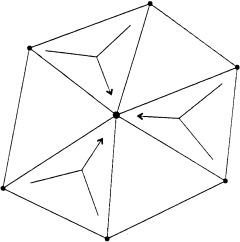
Local neighborhood defined around a given vertex. The contribution of every neighboring triangle must be considered in the distance update procedure.

Finally, the complete algorithm to compute d ${}_{\mathit{\text{g}}\text{(}\mathit{\text{S}}{}_{\text{▵)}}}$ (x ₁, x ₂) starts by initially letting d(x ₁) = 0, and then marching the solution upwards (using the procedure just described) until we reach x ₂.

Optimal weighted paths on triangulated surfaces

We have just described how to compute the weighted distance d ${}_{\mathit{\text{g}}\text{(}\mathit{\text{S}}{}_{\text{▵)}}}$(x ₁, x ₂) between two points on a triangulated surface. Moreover, because we have done this for all points on the triangulated surface outgrowing from x ₁ until we reached x ₂, we have the value of d ${}_{\mathit{\text{g}}\text{(}\mathit{\text{S}}{}_{\text{▵)}}}$(x ₁, x _p) for every x _p in the possible path between x ₁ and x ₂. We now describe how to compute the exact path (geodesic) that achieves this minimal distance d ${}_{\mathit{\text{g}}\text{(}\mathit{\text{S}}{}_{\text{▵)}}}$(x ₁, x ₂). The basic idea is once again to show that the geodesic curve C(s) holds [see Kimmel, 1999; Sethian, 1996c]:

(3)

In order then to compute the geodesic curve we have to back propagate from x ₂ in the direction given by −▿d. Following and improving on [Kimmel, 1999], we now describe a technique for numerically implementing this back propagation.

There exist many numerical methods to integrate the path resulting from equation (3). The first step is to construct an approximation for the distance function over every triangle. Based on this approximation we compute the gradient direction that gives the direction to follow in the minimizing path. The simplest approximation uses a linear interpolation, i.e., the distance function over each triangle is approximated by a plane determined by the distance values at its vertices. Standing at certain point P ₁ over the perimeter of a triangle, we compute the line segment along the gradient direction obtaining P ₂, the next point of the path (Fig. 6, left). When we are standing precisely at a vertex, as shown in Figure 6 (right), we have an estimate of the gradient direction for each neighboring triangle. In this case, we choose the one that gives the maximum gradient value in the downward direction, thus following the correct path.

Figure 6.

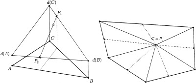
Building the path using a first order approximation of the distance function. Left: Situation when we are standing over one side of the triangle. Right: If we are standing precisely at a vertex (C), we have one gradient direction (dotted lines) for each neighboring triangle. We choose the one that gives the maximum gradient value in the downward direction.

Better approximations for the optimal path can be obtained using higher order approximations of the distance map. For example, in Kimmel [1999] a second order approximation (Heun's method) is given. Although it gives more accurate results, if the triangles are small enough, we have found that the first order approximation described above is sufficient.

As in the distance building algorithm, obtuse triangles must also be specially handled when finding geodesic paths. In this case, the distance function may present local minima causing the back propagation algorithm to stop prematurely. This problem is related to the introduction of the neighboring relation as previously mentioned. Issues regarding this problem and its solution are presented in Appendix C.2.

Having described the method for obtaining the geodesic path that achieves the minimum distance between two points, we now concentrate on the actual applications of these techniques.

Sulci and gyri detection

To detect sulci and gyri, we follow Khaneja et al. [1998] and search for valleys and crests on the 3D brain. Clearly, we will detect this by the search of paths minimizing

where f(·, ·) is a (positive) function of the surface principal curvatures κ₁, κ₂. For this, we use the technique described above (g ← f).

For example, to detect sulci, we search the deepest paths in the valleys, called the fund beds. Khaneja et al. [1998] do this by selecting

where κ_max is the maximal absolute principal curvature, and 𝒦 is the largest maximal curvature of the surface. Crests are similarly detected. In our case, we proceed differently and choose f to be a decreasing function of a certain creaseness/valleyness measure. This measure, inspired by the work of López et al. [1999] for Euclidean grids, is partially extended here to arbitrary triangulated domains.

López et al. [1999] classified and reviewed the most widespread crease and valley characterizations that have been proposed in literature. To determine the validity of the different characterizations, they devised a set of desirable properties referring to the clean and robust extraction of salient creases and valleys. Accordingly, they introduce a new creaseness/valleyness measure, which was shown to outperform existing ones. We now show the main idea and its extension to the 3D case at hand.

Instead of looking at maximal principal curvatures, we take the mean curvature value H as a creaseness/valleyness measure. As the mean curvature is an average of the principal curvatures, it should be more robust to noise. Over creases or valleys where one of the principal curvatures is locally maximum, its value will predominate in the averaging and this measure will caught the most relevant creaseness of the surface. We are left then to the computation of the mean curvature, described in the rest of this section.

Computations of any intrinsic geometrical properties from polygonal datasets require derivatives estimations to be computed from the given data. Several approaches can be taken in this respect. Approximation by an analytic surface is the most usual approach. In this case, an analytic surface is locally fitted to the input points, and the derivatives are computed for this approximating surface. Quadratic [Joshi et al., 1995; Khaneja et al., 1998; Taubin, 1995] and cubic [Samson and Mallet, 1997] patches were mostly used in the literature.

Another approach uses discrete estimation methods that are applied directly to the triangulated data and are based on polyhedral metrics. In this case, estimates for the mean and Gaussian curvatures are constructed directly from the given vertices [Desbrun et at., 1999; Krsek et al., 1998].

We have found that none of the above methods provide suitable approximations for arbitrary triangulation, so, inspired by the work of López et al. [1999] for Euclidean grids, we developed an alternative way to compute H on triangulated surfaces. The specific computation we propose is presented in Appendix D.

Having an adequate mean curvature estimation H (that we use as a creaseness/valleyness measure), we now select a particular weight function f, namely

(4)

where w is a positive constant, x is the creaseness/valleyness measure, and M = max ${}_{\mathit{\text{S}}{}_{\mathit{\text{▵}}}}$ {x}. As f is a decreasing function of x, it gives priority for advancing over high curvature zones (i.e., valleys or creases), and penalizes advancing over flat (low curvature) regions. Specifically, to search for creases we let x = H, prioritizing the advance over high positive curvature zones. For valleys we set x = −H, thus preferring high negative curvature values that correspond to deep valleys in the brain surface. Following the work by Cohen and Kimmel [1997], we can obtain an upper bound for the curvature of the resulting geodesic that is inversely proportional to the constant w. Therefore, if we want to control the regularity of the geodesic path (i.e., bound its maximum curvature value), we have to increase the constant w. Intuitively, if we increase w we are reducing the effect of the second term in the weight function f, that is, we are prioritizing the usual Euclidean distance term over the weighted one. This may avoid distance variations associated to the curvature dependent term giving a regularized geodesic path.

Boundary extraction

In this section, we briefly introduce another application of the techniques presented in this study: boundary detection of images defined over surfaces. This is a simple extension of the work in Cohen and Kimmel [1997], and is also available in our public domain software package. To detect edges, we must use weight values based on local image properties. As an example, we can choose as weights any decreasing function of the image gradient, which should take bigger values over flat regions (null gradient), and smaller values over high gradient zones. This way, the resulting path obtained from the back propagation algorithm should follow image boundaries as required.

Proceeding in the same manner as in the crease/valley extraction problem, we manually specify the start and end points along the boundary we want to extract. We compute the distance function starting at the first point, and applying the back propagation algorithm we found the geodesic curve joining the start and end points. The path thus obtained corresponds to the image boundary we are interested in.

Examples

We now present a number of results for our algorithm. As previously mentioned, the corresponding software package is available to the research community at http://www.ece.umn.edu/users/guille. The color figures presented here can be viewed in the online issue available at the Wiley InterScience site.

Figure 7 presents the first brain used in our examples (left), and a geodesic curve with its corresponding distance. Here we used g ≡ 1. The geodesic distance provides the true distance between the two marked points and the geodesic curve the path to be traveled on the surface to achieve this minimal geodesic distance.

Figure 7.

Left: Triangulated data for brain 1. The surface contains 63000 triangles and 31500 points. Center: Geodesic curve obtained with g = 1. Right: Distance values rendered over the surface. Color values range from red (zero distance) to blue (largest distance values).

Figure 8 shows the first example of the detection of sulci and gyri with the approach here presented. In this case, a crease (gyri) is shown. Additional examples are given in Figure 9.

Figure 8.

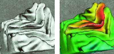
Crease extraction for brain 1. Left: Crease line shown over the original surface. Right: Crease line shown over the curvature‐weighted distance function rendered over the surface.

Figure 9.

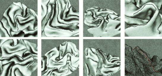
Additional examples of crease extraction for brain 1. The last figure shows the crease line over the triangulated mesh.

In Figure 10 we show the computation of valleys (bottom of sulci). Additional examples are given in Figure 11.

Figure 10.

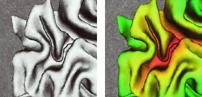
Valley extraction for brain 1. Left: Valley line shown over the original surface. Right: Valley line shown over the curvature‐weighted distance function rendered over the surface. Color reference as before.

Figure 11.

Additional examples of valley extraction for brain 1.

Figure 12.

Left: Triangulated data for brain 2. The surface contains 7700 triangles and 3800 points. Center: Geodesic curve obtained with g = 1. Right: Distance values rendered over the surface. Color reference as before.

Figure 13.

Crease extraction for brain 2.

Figure 14.

Valley extraction for brain 2.

Figure 15.

Additional valley extraction example for brain 2. Left: Valley line shown over the original surface. Center: Corresponding weighted distance values are rendered over the surface. Right: The distance function is only computed until we reach the selected end point, thereby further improving the computational time. Color reference as before.

The following set of the figures in this study repeats this for additional, lower resolution, brain data obtained from Khaneja et al. [1998].

DISCUSSION

In this study, we have described a public domain software package for the computationally optimal generation of curves on 3D brain surfaces. The system can be used for a number of applications in computational neuroscience, including brain flattening and brain warping. The package concentrates on triangulated surfaces, whereas its extension to implicit surfaces will be reported elsewhere.

Other works have been reported in the literature on automatic computation of important 3D curves on brain surfaces. We review a few representative works and compare them with our approach presented here. The interested reader is referred to the works mentioned below for additional details and further literature on the subject.

As mentioned before, many authors use Dijkstra and variations of it to compute geodesics on triangulated surfaces, and the problems with this approach were already described. As also stated above, our work is inspired by Khaneja et al. [1998], which similarly to our approach, requires the user to mark the two end points of the curve of interest. A number of works for fully automatic detection (and modeling) of sulci regions and other curves of interest in 3D brain images have been reported [Thirion and Gourdon, 1993; Vaillant et al., 1996; Le Goualher et al., 1998, 1999; Manceaux‐Demiau et al., 1998].

Thirion and Gourdon [1993] present a very interesting approach where the crest lines are computed as the intersection of two iso‐surfaces, one defining the 3D surface of the brain and a second one defining a measurement of creaseness. In contrast with ours, this technique is fully automatic, though due to the lack of user control, it might result in spurious curves or non‐connected ones.

Le Goualher et al. [1998, 1999] propose a series of very efficient geometric operations to detect the sulci median surface, also without user intervention. First, they combine morphological filtering for closing sulci walls, together with analysis of the curvature sign. They assume that the sulci are convex entities, which is not always the case for high resolution data, and then they can not be precisely defined just by the sign of curvature, as suggested by the authors. A thinning algorithm is then applied, followed by active surfaces. These steps can not automatically guarantee that the detected curves and surfaces are topologically correct. A related approach is described in Vaillant et al. [1996]. Note that these studies are not just interested in finding the sulci bed, but on modeling the folds and the complete sulci, a goal beyond the one in this study. Using their approach modeling can also be done after the detection performed with our technique.

In general, automatic procedures like those mentioned above has the advantage of eliminating the user intervention. On the other hand, as expected, they are less robust. Robustness is traded‐off by automatization. Moreover, as explained before, the technique proposed here is computationally optimal. The selection of the specific technique depends on the application. First, note that our technique is robust to errors in the selected end points, meaning that small errors in their position do not significantly affect the geodesic path. Second, in a number of applications the end points can be easily detected, like in brain flattening, where all the grid points are to be used. Third, in applications like brain warping, many users prefer to have control on the selection of the sulci and gyri used for boundary conditions of their differential maps, and the tool here presented brings a step forward from the current fully manual tracing technique being used. Nevertheless, extending the technique presented here to a fully automatic procedure will bring the best of both worlds and is of great interest. The basic direction is to automatically select two or more points that belong to the same crest or valley, and then apply the algorithm here discussed to connect between them. The search for these points can, for example, be done based on the automatic techniques just discussed. This is the subject of current research.

APPENDIX A.

Basic differential geometry

For completeness, we present the basic definitions of 3D curvatures and geodesic curves; for an extensive treatment of 3D differential geometry, see Do Carmo [1959]. We consider regular surfaces S(u, v) = (x(u, v), y(u, v), z(u, v)): IR ² → IR ³ that are homeomorphisms, for which each one of the coordinates have continuous partial derivatives, and such that the differential map is one‐to‐one. These regularity conditions avoid self‐intersections unexpected in 3D data of the brain. We define the tangent vectors (subscripts indicate derivatives)

Any vector tangent to the surface S defines the tangent plane, and can be obtained as a linear combination of these two vectors. Every vector in the tangent plane it is the tangent to a parametrized curve C(p) ∈ S(u(p), v(p)) going through the point P (p is an arbitrary parametrization); see Figure 16.

Figure 16.

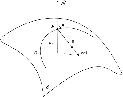
Basic 3D geometry and curvatures.

The unit normal to the surface is given by

where (· × ·) stands for the vector obtained by the exterior product of two vectors (Fig. 16).

Let C be a curve on S passing through P, κ the curvature of C at P, and cos θ = 〈n→,

〉 where n→ is the normal to the curve and

as before the normal to the surface (both at the point P) (Fig. 16). The number κ _n = κ cos θ is called the normal curvature of C at P. The normal curvature is basically the length of the projection of κn→ over the surface normal. All curves lying on the surface and having at a given point the same tangent, have the same normal curvature, meaning that the normal curvature is a property intrinsic to the surface and not to the specific curve.

From the results above, we can talk about the normal curvature at a given direction. We can then consider all possible directions, and obtain the maximal and minimal normal curvatures κ₁ and κ₂, respectively. These are the principal curvatures of the surface and the corresponding directions are the principal directions. This leads to the definition of the Gaussian curvature:

and the mean curvature

Let's now present a slightly different way of computing the mean curvature H that which is used in this study. If we locally define the surface as a function z = f(x, y), then taking F(x, y, z) = z − f(x, y) = 0, the mean curvature can be obtained as

The surface normal can be expressed in terms of ▿F as

where

is the outward unit normal. Therefore, we can compute the mean curvature as the divergence of the normal vector:

The last concept we want to introduce is the concept of geodesic curvature. The geodesic curvature κ_g at a point P of a curve C ∈ S is given by the projection of the vector κn→ onto the tangent plane (this is the absolute value). That is, the absolute value of the geodesic curvature is equal to the length of the tangential component of κn→. From this, it is obvious that

A geodesic curve is a curve on the surface with zero geodesic curvature. The minimal path between two points on a surface is always a geodesic curve.

APPENDIX B.

Update procedure for a single triangle

The first part of the global distance computation is how to locally propagate the distance inside a given triangle, when some of the vertices of this triangle have already been assigned a distance and some not. Consider the triangle ABC, as shown in Figure17. Here we want to update the distance value at vertex C. The idea is to fit a plane over the triangle, given the distance values at the other two vertices d(A) and d(B), and the slope g (corresponding to the right hand side of the Eikonal equation (2)). We assume without loss of generality that d(A) = 0.

Figure 17.

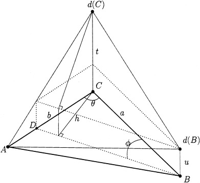
Update procedure for triangle ABC. We want to compute the distance value at C, fitting a plane over the triangle, based on A and B distances, and the desired plane slope g. We require the solution t to be greater than u, and to be updated from within the triangle, that is, h should lay between edges CA and CB.

We define the following quantities:

Then, we search for t that sets the slope of the plane to be:

Substituting h in the previous expression we obtain a quadratic equation for t (see Kimmel and Sethian [1998] and Sethian [1996c] for the exact derivation):

(5)

The solution t must be greater than u, and should be updated from within the triangle, that is, h should lay between edges CA and CB (Fig. 17). When h coincides with CA we obtain the lower bound CD = a cos θ. Similarly, when h coincides with CB, we have the upper bound . By similarity, we have t/b = u/AD, so CD = b − AD = b − b u/t = b(t − u)/t.

Thus, the resulting restriction for the update to come from inside the triangle becomes

(6)

The update procedure for a vertex over one triangle is then given by:

• 1Compute t from equation (5).
• 2If t > u and condition (6) is satisfied: then d(C) = min{d(C), t + d(A)} else d(C) = min{d(C), bg + d(A), ag + d(B)}

APPENDIX C.

C.1. Handling non‐acute triangulations in the distance algorithm

The nature of the upwind operators used by the distance algorithm described in Appendix B guarantee that the solution is built in a monotonous fashion. Nonetheless, the splitting strategy for obtuse triangles mentioned earlier can lead to situations in which the marching procedure suddenly finds a smaller distance value than a previously computed one. For example, consider a simple situation like the one in Figure18.

Figure 18.

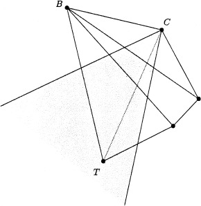
Undesirable situation caused by splitting obtuse triangles. See text for explanation.

Suppose that the update procedure is approaching by the lower‐left side of the figure, where we have just computed the final distance values for vertices T and B, in that order (i.e., d(T) < d(B)). Assuming that B was updated from T, we have d(B) = d(T) + TB (for simplicity, we assume that the update comes directly along the direction of BT). Next, we proceed to compute the distance at C. As we have an obtuse angle at C we must find the appropriate vertex in the unfolded surface, corresponding to T (as seen earlier). If CT < BT we may find a value for d(C) satisfying d(C) < d(B), contrary to the upwind nature of the method. If we have uniform weights, the value at B remains correct, because the update of B from T (d(B) = d(T) + TB) is always smaller than the update of B from C (d(B) = d(C) + CB = d(T) + TC + CB > d(T) + TB), just using the triangular inequality TC + CB > TB. On the other hand, if weights are non‐uniform (as is our case) the mentioned inequality does not hold anymore, and we may find a smaller value for d(B) if its update comes from vertex C. For example, suppose that the cost to reach B is much higher than the one to reach C. In this situation, it may be cheaper to reach B via C, than going directly from T to B, thus obtaining a smaller value for d(B).

Situations like this cause the algorithm to obtain smaller distance values than previously computed ones, in contradiction with the monotonous construction procedure intended by fast marching methods. The cause of this problem is the previously mentioned unilateral neighboring relationship that exists between C and T; T is C's neighbor, but C is not T's neighbor. So, when we update the neighbors of T, we do not consider C, when we actually should.

In the implementation of the algorithm, any time a situation like this arose, we recompute distances at all vertices with greater distance values than the newly computed one. Doing this, we guarantee monotony in the construction procedure, as initially intended. In practice, only immediate neighboring vertices can be affected, and we have found enough and much faster to recompute distances only at these vertices.

C.2. Handling non‐acute triangulations in the back propagation algorithm

If we consider the distance map d ${}_{\mathit{\text{g}}\text{(}\mathit{\text{S}}{}_{\text{▵)}}}$(x ₁, x ₂) for any x ₁, x ₂ ∈ S _▵, it should have only one minimum (global minimum) corresponding to the point x ₁ having zero distance. The splitting strategy for obtuse triangles used in the construction procedure of the distance function may produce local minima, however, causing the back propagation algorithm to stop prematurely. Kimmel (personal communication), pre‐processes the triangulated surface to eliminate all problems with obtuse triangles, both the ones reported when building distances and the ones discussed here. This pre‐processing is done to the whole surface, not just to the triangles that will actually be used in the computation, because this is not known a priori. We have opted for the techniques here described that handles obtuse triangles on the fly, as required by the computed path.

Such local minima does not actually exist, but we may have situations like the one in Figure 19 where we show a local neighborhood around vertex C. As the angle

is obtuse, we must consider the corresponding vertex T in the unfolded surface.

Regarding Figure 19, suppose that d(C) is smaller than any of its direct neighbors, and d(T) < d(C). It can be easily proven that a situation like this can actually occur as a result of the distance construction method. In this situation, once we reach vertex C it appears as a local minima (within its direct neighbors), and the back propagating algorithm would fail (see Fig. 19, left). Instead, we have to see further and consider the new neighboring relationship existing between vertices C and T, leading to the situation shown in Figure 19 (right), where two new triangles are added as neighbors. This way, we now follow the correct path, traversing through the unfolded surface toward the minimum.

Figure 19.

Handling obtuse triangles in the back propagation algorithm. Left: Considering the shown neighborhood leads to the local minima situation. Right: Neighborhood that gives the correct path through the unfolded surface.

APPENDIX D.

Computation of the mean curvature H

First (as described in Appendix A) we compute the mean curvature as the divergence of the normal vector:

(7)

where

is the outward unit surface normal.

Consider an oriented surface 𝒜 with closed boundary δ𝒜; by the divergence theorem (see Lee [1997] for example) we have

where n→ is the outward unit normal to the curve δ𝒜, whose length element is dl.

We now consider the following approximation for the mean curvature

(8)

The discrete version of equation (8), when we have a triangulated surface S _▵, becomes

(9)

where p is the number of neighbors of the current vertex, and A is the local surface area, computed as the sum of areas of all triangles sharing the central vertex (Fig. 20).

The sum in equation (9) is computed along the polygonal curve δ𝒜, as shown in Figure 20. Surface normals

are naturally associated to each vertex, and are computed using common normal estimation procedures over triangulated surfaces. Curve normals n→_i are only defined along the sides of the polygonal curve. To estimate its value at the vertices we average the normals from both sides of the curve.

Intuitively, if all points in a local neighborhood are coplanar, the products

in equation (9) vanish and we have H = 0. Now, if we pull up the central point in Figure 20 (as

becomes closer to n→_i) these products start growing, giving higher values for H.

Figure 20.

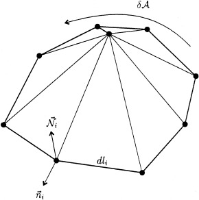
Three dimensional view of the triangulated surface element considered to compute the mean curvature using equation (9).

Note that the proposed approximation for the mean curvature has a well defined dynamic range, namely, which remains fixed once the triangulation is given. This is a desirable property, that avoids having outliers in the curvature values, being particularly important when dealing with arbitrarily triangulated data.

REFERENCES

- Angenent S, Haker S, Tannenbaum A, Kikinis R (1998): Laplace‐Beltrami operator and brain flattening. University of Minnesota ECE Report. [DOI] [PubMed]
- Barth TJ, Sethian JA (1998): Numerical schemes for the Hamilton‐Jacobi and level set equations on triangulated domains. J Comp Physics 145: 1–40. [Google Scholar]
- Bertalmio M, Sapiro G, Randall G (1999): Region tracking on level‐sets methods. IEEE Trans Med Imaging 18: 448–451. [DOI] [PubMed] [Google Scholar]
- Bruckstein AM (1988): On shape from shading. Comp Vision Graph Image Process 44: 139–154. [Google Scholar]
- Caselles V, Kimmel R, Sapiro G, Sbert C (1997): Minimal surfaces based object segmentation. IEEE‐PAMI 19: 394–398. [Google Scholar]
- Cheng LT, Burchard P, Merriman B, Osher S. (2000): Motion of curves constrained on surfaces using a level set approach. UCLA CAM Report 00‐32.
- Cohen LD, Kimmel R (1997): Global minimum for active contours models: a minimal path approach. Intl J Comp Vision 24: 57–78. [Google Scholar]
- Desbrun M, Meyer M, Schroder P, Barr AH (1999): Implicit fairing of irregular meshes using diffusion and curvature flow. Computer Graphics (SIGGRAPH '99). p 317–324.
- Do Carmo MP (1976): Differential geometry of curves and surfaces. New Jersey: Prentice‐Hall. [Google Scholar]
- Dijkstra E (1959): A note on two problems in connection with graphs. Numerische Math 1: 269–271. [Google Scholar]
- Faugeras O, Clément F, Deriche R, Keriven R, Papadopoulo T, Gomes J, Hermosillo G, Kornprobst P, Lingrad D, Roberts J, Viéville T, Devernay F (1999): The inverse EEG and MEG problems. The adjoint state approach I: the continuous case. Inria Research Report 3673.
- Grenander U, Miller M (1998): Computational anatomy: an emerging discipline. Quarterly Appl Math LVI: 617–694. [Google Scholar]
- Helmsen J, Puckett EG, Collela P, Dorr M (1996): Two new methods for simulating photolithography development in 3D. Proc SPIE Microlithography IX: 253. [Google Scholar]
- Joshi M, Cui J, Doolittle K, Joshi S, Lanterman A, Wang L, Miller M (1999): Brain segmentation and the generation of cortical surfaces. Neuroimage 9: 461–476. [DOI] [PubMed] [Google Scholar]
- Joshi SC, Wang J, Miller MI, Van Essen D, Grenander U (1995): On the differential geometry of the cortical surface. Proceedings of SPIE 1995 Geometric Methods in Applied Imaging, San Diego, CA, 9–14 July.
- Khaneja N, Miller MI, Grenander U (1998): Dynamic programming generation of geodesics and sulci on brain surfaces. IEEE Trans Pattern Analysis Machine Intelligence 20: 1260–1265. [Google Scholar]
- Kiebel SJ, Friston KJ (2000): Characterization of PET data using anatomically informed basis functions. Human Brain Mapping 2000, San Antonio, Texas, June 12–16.
- Kimmel R (1999): Numerical geometry of images: theory, algorithms, and applications. Technion CIS Report 9910.
- Kimmel R, Sethian JA (1998): Computing geodesic paths on manifolds. Proc Natl Acad Sci 95: 8431–8435. [DOI] [PMC free article] [PubMed] [Google Scholar]
- Krsek P, Lukás G, Martin RR (1998): Algorithms for computing curvatures from range data In: Cripps R. (ed.). The mathematics of surfaces VIII. Birmingham: Information Geometers Limited, p 1–16. [Google Scholar]
- Lafon F, Osher S (1996): High order two‐dimensional nonoscillatory methods for solving Hamilton‐Jacobi scalar equations. J Comput Phys 123: 235–253. [Google Scholar]
- Le Goualher G, Collins DL, Barillot C, Evans AC (1998): Automatic identification of cortical sulci using a 3D probabilist atlas. Proc MICCAI '98, October. Cambridge, MA: Springer‐Verlag; p 509–518. [Google Scholar]
- Le Goualher G, Procyk E, Collins DL, Venugopal R, Barillot C, Evans AC (1999): Automated extraction and variability analysis of sulcal neuroanatomy. IEEE Trans Med Imaging 18: 206–217. [DOI] [PubMed] [Google Scholar]
- Lee JM (1997): Riemannian manifolds: an introduction to curvature. New York: Springer‐Verlag. [Google Scholar]
- López AM, Lumbreras F, Serrat J, Villanueva JJ (1999): Evaluation of methods for ridge and valley detection. IEEE Trans Pattern Anal Machine Intelligence 21: 327–335. [Google Scholar]
- Manceaux‐Demiau A, Bryan RN, Davatzikos C (1998): A probabilistic ribbon model for shape analysis of the cerebral sulci: application to the central sulcus. J Comp Assist Tomogr 22: 962–971. [DOI] [PubMed] [Google Scholar]
- Mémoli F, Sapiro G (2001): Fast computation of weighted distance functions and geodesics on implicit hyper‐surfaces. IMA University of Minnesota Technical Report 1754.
- Mitchell JSB (1988): An algorithmic approach to some problems in terrain navigation. Artif Intell 37: 171–201. [Google Scholar]
- Mitchell JSB, Payton D, Keirsey D (1987): Planning and reasoning for autonomous vehicle control. Intl J Intell Sys 2: 129–198. [Google Scholar]
- Osher S, Fedkiw RP (2000): Level set methods. UCLA CAM Technical Report 00‐08.
- Osher SJ (1993): A level‐set formulation for the solution of the Dirichlet problem for Hamilton‐Jacobi equations. SIMA J Num Anal 24: 1145. [Google Scholar]
- Osher SJ, Sethian JA (1988): Fronts propagation with curvature dependent speed: algorithms based on Hamilton‐Jacobi formulations. J Comput Phys 79: 12–49. [Google Scholar]
- Rouy E, Tourin A (1992): A viscosity solutions approach to shape‐from‐shading. SIAM J Num Anal 29: 867–884. [Google Scholar]
- Samson P, Mallet J (1997): Curvature analysis of triangulated surfaces in structural geology. Math Geol 29: 391–412. [Google Scholar]
- Sapiro G (2001): Geometric approaches for functional MRI Analysis In: Yan H. (editor). Signal processing for magnetic resonance imaging and spectroscopy. New York: Marcel Decker; (in press). [Google Scholar]
- Sethian JA (1996a): Fast marching level set methods for three‐dimensional photolithography development. Proc SPIE International Symposium on Microlithography, Santa Clara, CA, March.
- Sethian JA (1996b): A fast marching level‐set method for monotonically advancing fronts. Proc Natl Acad Sci 93: 1591–1595. [DOI] [PMC free article] [PubMed] [Google Scholar]
- Sethian JA (1996c): Level set methods: evolving interfaces in geometry, fluid mechanics, computer vision and materials sciences. Cambridge, UK: Cambridge University Press. [Google Scholar]
- Taubin G (1995): Estimating the tensor of curvature of a surface from a polyhedral approximation. Proceedings of the 5th International Conference on Computer Vision (ICCV). Cambridge, MA: MIT; p 902–907. [Google Scholar]
- Teo P, Sapiro G, Wandell B (1997): Creating connected representations of cortical gray matter for functional MRI visualization. IEEE Trans Med Imaging 16: 852–863. [DOI] [PubMed] [Google Scholar]
- Thirion JP, Gourdon A (1993): The marching lines algorithm: new results and proofs. INRIA TR 1881: 1. [Google Scholar]
- Toga AW (1998): Brain warping. New York: Academic Press. [Google Scholar]
- Thompson P, Woods R, Mega M, Toga A (2000): Mathematical/computational challenges in creating deformable and probabilistic atlases of the human brain. Hum Brain Mapp 9: 81–92. [DOI] [PMC free article] [PubMed] [Google Scholar]
- Tsitsiklis JN (1995): Efficient algorithms for globally optimal trajectories. IEEE Trans Automatic Control 40: 1528–1538. [Google Scholar]
- Vaillant MA, Davatzikos C, Bryan RN (1996): Finding 3D parametric representations of the deep cortical folds. Proceedings of the IEEE Workshop Mathematical Methods in Biomedical Image Analysis, June. San Francisco, CA: IEEE Computer Society Press; p 151–159. [Google Scholar]
- Van Essen DC, Drury H, Joshi S, Miller MI (1998): Functional and structural mapping of human cerebral cortex: solutions are in the surfaces. Proc Natl Acad Sci 95: 788–795. [DOI] [PMC free article] [PubMed] [Google Scholar]
- Wandell B, Chial S, Backus B (2001): Visualization and measurement of the cortical surface. J Cogn Neurosci 12: 739–752. [DOI] [PubMed] [Google Scholar]
- Wandell B, Engel S, Hel‐Or H (1996): Creating images of the flattened cortical sheet. Invest Opth Vis Sci 36: S612. [Google Scholar]
- Yezzi A, Kichenassamy S, Olver P, Tannenbaum A (1997): Geometric active contours for segmentation of medical imagery. IEEE Trans Medical Imaging 16: 199–210. [DOI] [PubMed] [Google Scholar]
- Zigelman G, Kimmel R, Kiryati N (2000): Texture mapping using surface flattening via multidimensional scaling. Technion‐CIS Technical Report 2000–01.