Lesion segmentation and manual warping to a reference brain: Intra‐ and interobserver reliability

Abstract

The study of subjects with acquired brain damage has been an invaluable tool for exploring human brain function, and the description of lesion locations within and across subjects is an important component of this method. Such descriptions usually involve the separation of lesioned from nonlesioned tissue (lesion segmentation) and the description of the lesion location in terms of a standard anatomical reference space (lesion warping). The objectives of this study were to determine the sources and magnitude of variability involved in lesion segmentation and warping using the MAP‐3 approach. Each of two observers segmented the lesion volume in ten brain‐damaged subjects twice, so as to permit pairwise comparisons of both intra‐ and interobserver agreement. The segmented volumes were then warped to a reference brain using both a manual (MAP‐3) and an automated (AIR‐3) technique. Observer agreement between segmented and warped volumes was analyzed using four measures: volume size, distance between the volume surfaces, percentage of nonoverlapping voxels, and percentage of highly discrepant voxels. The techniques for segmentation and warping produced high agreement within and between observers. For example, in most instances, the warped volume surfaces created by different observers were separated by less than 3 mm. The performance of the automated warping technique compared favorably to the manual technique in most subjects, although important exceptions were found. Overall, these results establish benchmark parameters for expert and automated lesion transfer, and indicate that a high degree of confidence can be placed in the detailed anatomical interpretation of focal brain damage based upon the MAP‐3 technique. Hum. Brain Mapping 9:192–211, 2000. © 2000 Wiley‐Liss, Inc.

INTRODUCTION

One approach for exploring the relationship between brain structure and function has been the cognitive and behavioral investigation of subjects with acquired brain damage. New brain imaging techniques allow regions of brain damage in human subjects to be represented at increasingly higher spatial resolution, and interactive graphic interfaces provide new tools for viewing and manipulating these images. As the neuroanatomical data derived from the study of brain‐damaged subjects become more precise, it is essential to understand the sources and magnitude of variability inherent in the identification of lesion boundaries and the transfer of these boundaries into standard anatomical spaces. However, few studies of the precision and reliability of the assignment of lesion location to a standard space have been performed. The objectives of this study are to determine the magnitude and sources of variability involved in lesion segmentation and warping to estimate how reliably lesions can be located within and across subjects.

Lesion segmentation

The identification of lesion boundaries requires discriminations between different types of tissue (grey matter, white matter, cerebral spinal fluid, lesioned tissue) based upon voxel intensity values. These discriminations can be difficult to make, because the intensity values overlap for different types of tissue. This is one reason that the development of computational algorithms for the automatic segmentation of abnormal tissue is still an active area of research [e.g., see Bedell et al., 1997; Bendszus et al., 1997; Dastidar et al., 1999; Soltanian‐Zadeh et al., 1998]. An advantage of manual segmentation procedures, such as tracing the contours of a lesion by hand, is that knowledge about surrounding neuroanatomical features and the contiguity and smoothness of the lesion can aid the decision‐making process. For instance, in T1‐weighted MR images, the voxel intensity values of lesioned tissue can overlap with those of grey matter, and, hence, the assignment of voxels with such ambiguous intensity values depends in part upon their position relative to other structural features, such as whether they are located at the edge or in the center of a gyrus. A disadvantage of manual procedures is their reliance upon subjective judgments, which raises the possibility that different observers will reach different conclusions about the presence or absence of lesioned tissue, or even that the same observer will reach different conclusions on different occasions. The principal objective of this study is to examine the sources and magnitude of the variability in delineating the borders of a lesion.

Lesion warping

Once lesion boundaries are identified, a second issue is how to compare lesion locations across subjects. Although qualitative descriptions are used frequently (e.g., “all subjects had damage to the left inferior frontal gyrus”), more precise image‐based quantitative descriptions across a group of subjects necessitate warping the lesions from individual subjects into a standard anatomical space. Neuroanatomical comparisons across brain‐damaged subjects have relied extensively upon manual warping techniques, in which a lesion is mapped onto a standard template using structural features, such as sulci and gyri, as guides. In the past, standard templates were most often sets of two‐dimensional brain images acquired in single orientation. Lesions were transferred onto these templates, and the results were described qualitatively or quantitatively according to regions of interest [e.g., see Damasio and Damasio, 1980; Kunesch et al., 1995; Naeser and Hayward, 1978; Woods et al., 1993, and many others].

We have recently developed a technique, known as the MAP‐3 technique, that allows lesion volumes to be manually warped to a three‐dimensional reference brain, and then analyzed quantitatively in much greater detail than previously possible [Frank et al., 1997]. The technique is a two‐step procedure that involves: (1) manually adjusting the orientation and amount of tissue covered by each section in a reference brain to match a lesioned brain, and (2) delineating the boundaries of the tissue volume in the reference brain that is isomorphic to the damaged tissue volume in the lesioned brain. In contrast to automated or semiautomated warping procedures, the MAP‐3 technique involves a large number of subjective decisions, and it is possible that different observers could warp the same lesion very differently. A second objective of this study was to determine the interobserver agreement in warped volume size and location, because the utility of the technique rests in large part upon the degree to which different observers generate similar isomorphic warped lesion volumes.

In many functional neuroimaging studies, a similar need to draw neuroanatomical conclusions across groups of subjects has led to the development of automated and semiautomated warping procedures. For example, one common approach has been to warp the data into the space of Talairach and Tournoux atlas [Talairach and Tournoux, 1988] through the subjective identification of the anterior and posterior commissures, followed by linear scaling along a few dimensions (e.g., brain width, length, and height) [e.g., see Fox et al., 1985, 1988; Friston et al., 1991; Sorlie et al., 1997]. More recently, computational algorithms have been developed that compute a “best fit” between two images by adjusting the values of a set of linear and nonlinear scaling and rotation parameters to minimize the variance across two images [e.g., see Christensen et al., 1997; Schormann and Zilles, 1998; Woods et al., 1998a, b]. Such automated and semiautomated techniques have been used very successfully in normal subjects to increase the signal‐to‐noise ratio of functional images, and to identify regions of activation that are common across subjects and studies.

Automated warping techniques such as those used in functional neuroimaging studies may be less appropriate for studies using brain‐damaged subjects, for two reasons. First, there may be no compensation for the structural distortions introduced by a lesion (e.g., ventricular enlargement, large regions of atypical voxel intensity values, etc.). Second, there may be inadequate correction for anatomical variability between subjects. Whereas anatomical variability is an issue in functional neuroimaging studies as well, it is of particular concern for studies using the lesion method because the lesion technique often relies upon a combination of information about both group tendencies and individual variability. For instance, emphasis is often placed on how many of the individual subjects with damage to a particular region show particular cognitive deficits. If the warping technique does not take local anatomical structure into account, a subject may fail to show the expected deficits either because the lesion‐behavior correspondence is abnormal, or more trivially because the fit into the standard space is poor and, hence, the lesion is not localized to the appropriate neuroanatomical structure. Whereas these are important theoretical issues, the degree to which they influence the warping of lesions into a reference space and subsequently affect the interpretation of lesion locations has not been examined. A third objective of this study is to compare the results from the MAP‐3 warping procedure to an automated warping technique based upon AIR‐3 [Woods et al., 1998a, b]. AIR‐3 is a multiparameter image registration algorithm that has been used widely in functional neuroimaging studies to remove movement artifacts, to register functional and anatomical images, and to warp functional and anatomical images into a standard reference space. The purpose of our comparisons was to determine whether automated techniques may be acceptable substitutes for more time‐consuming manual techniques, and to establish benchmarks or indices with which to measure the performance of improved algorithms in the future.

One benefit of lesion warping is that it permits volumetric statistical parametric maps to be created across warped lesion volumes; these maps can be used to provide quantitative structure–function correlations across a group of brain‐damaged subjects. For example, volumetric maps have been used to map out the location of maximal lesion overlap across a group of subjects, or to highlight the location of those lesions that are associated with the largest deficits in behavioral performance. The analysis of individual warped volumes can provide information about the variability to be expected in transferring any single volume into a standard reference space. However, such analysis provides little information about how individual variability affects volumetric statistical maps based upon intersubject comparisons of the warped volumes. A fourth objective of this study is to assess the agreement between lesion overlap maps created from different observers and techniques to determine whether volumetric maps are robust to variability at the level of individual warped lesion volumes.

In summary, the objectives of this study are to determine the sources and magnitude of variability involved in lesion segmentation and warping. For lesion segmentation, intra‐ and interobserver comparisons will be made across lesion volumes segmented from the same subject. For lesion warping, interobserver comparisons will be made across lesion volumes generated by warping a subject's lesion into standard reference brain using the MAP‐3 manual warping technique, and across volumes generated with the MAP‐3 vs. an automated (AIR‐3) warping technique. Agreement in the size and location of the volumes segmented and warped by different observers and techniques will be assessed using a set of four quantitative measures.

Although lesion segmentation and warping procedures have been used successfully as tools for understanding the relationship between brain structure and brain function, the precision of these tools has rarely been investigated. The information which will be gained from a careful evaluation of segmentation and warping procedures should bear upon several important questions. First, it should establish an upper‐bound on the accuracy of the technique to determine an appropriate level of scale for correlating structure and function with lesion method. Second, it should provide measures that can be used to identify subjects in whom the lesion is particularly difficult to segment or warp without ambiguity, so that the degree of confidence placed in their data can be weighted appropriately. Third, it should provide human benchmark performance measures that can be used to evaluate automated segmentation and warping procedures.

METHODS

Image dataset

Structural brain images were obtained from ten subjects with left frontal brain damage caused by ischemic events. Subjects were selected to have lesions in the same general area to permit the construction of meaningful volumetric statistical maps from the warped lesion volumes. The subjects were drawn from the Patient Registry of the Division of Behavioral Neurology and Cognitive Neuroscience at the University of Iowa. Informed consent was obtained from all subjects, using procedures that were approved by the University of Iowa Institutional Review Board.

For each subject, T1‐weighted magnetic resonance (MR) images were obtained with a General Electric Signa scanner operating at 1.5 T. A set of 124 contiguous coronal slices with an interpixel distance of 0.94 mm and a thickness of 1.5 mm was obtained for all but one subject (thickness of 3.0 mm in 1496jb) using the following protocol: SPGR/50, TR24, TE5, NEX2, FOV 24 cm, matrix 256 × 192. All results are given in terms of voxels. The larger voxel size for 1496jb may minimize the observer differences in segmentation and warping in this subject, because many of the transitions between tissue types (e.g., lesioned vs. nonlesioned) will be marked by less fine, but possibly more distinguishable, differences in voxel intensity values.

Segmentation of lesion volumes and transfer to a reference brain

Equipment.

All image processing and analysis was performed with Silicon Graphics Workstations (Silicon Graphics, Mountain View, CA). Neuroanatomical analysis of MR images was performed using Brainvox, a three‐dimensional interactive rendering package [Damasio and Frank, 1992; Frank et al., 1997]. All computations upon the segmented and warped lesion volumes were performed using a suite of modular software utilities that support pixelwise image computations [Frank et al., 1997].

Segmentation of lesion volumes.

For each subject, the boundaries of the lesion were manually traced on all contiguous coronal sections in which the lesion was judged to be present, using a mouse‐controlled cursor and Brainvox. Whereas all tracing was performed on the originally acquired coronal sections, each observer was allowed to freely take advantage of the interactive nature of Brainvox to permit better identification of the lesion boundaries. This included reslicing the brain volume at multiple orientations for comparison to the coronal section, interactively mapping user‐defined areas across multiple 2D and 3D views of the brain, and adjustments to the image contrast level to better distinguish between cerebral spinal fluid, gray matter, white matter, and lesioned tissue. This freedom was appropriate for the goals of this study: establishing “usage rules” or predetermined values would not resolve underlying sources of ambiguity, and would thus artificially reduce the amount of variance that arises during manual segmentation procedures.

The lesion in each subject was traced four times: twice by an observer with good neuroanatomical knowledge but with less than 10 hr of lesion‐tracing experience (JF), and twice by a highly experienced observer with over 15 years of experience with lesion segmentation and warping (HD). At least 2 months separated the tracings performed by each observer, and each observer was blind to all previous traces and image adjustments. For each tracing, the corresponding segmented lesion volume was computed as all voxels within and including the boundaries traced across all coronal sections. The two separate volumes segmented by each observer were used to assess intraobserver reliability, and the first volumes segmented by the observers were used to compute the interobserver reliability. Differences in the size and contours of the segmented volumes were evaluated using a set of volumetric comparison measures that are described below.

MAP‐3 manual warping.

Lesions were manually transferred to a normal reference brain using the MAP‐3 technique [for details, see Frank et al., 1997], which is illustrated graphically in Figure 1. The MAP‐3 technique is implemented within the Brainvox software package by a human observer. It begins with a manual rigid‐body reorientation of a reference brain to a source brain based on visual comparison of the structural features (especially sulci) between the two brains, followed by a manual transfer of the lesion boundary from the source to the reference brain. In brief, for each lesion transferred, the normal reference brain MR volume was first resliced to match the slices of the lesioned brain MR volume, thus creating the best possible correspondence between the coronal slices in the lesioned brain and the resliced normal reference brain in terms of the three‐dimensional slice orientation and the percentage of brain volume contained in each slice. Next, the contour of the lesion on each slice was transposed onto the matched slices of the normal brain, taking into consideration anatomical landmarks (e.g., whether the lesion extended medially beyond the fundus of the precentral gyrus). The traces transferred to the normal reference brain were used to define an isomorphic volume in the reference brain. Differences in the size and contours of the warped volumes were evaluated using a set of volumetric comparison measures that are described below.

Figure 1.

Steps involved in creating a MAP‐3 transfer volume. First, the normal reference brain is examined to select an orientation and anterior‐posterior extent that corresponds to the orientation and the extent of the lesioned tissue in the damaged brain; this step can be appreciated graphically by comparing the tissue between the black lines on the 3D rendered lesioned brain (brain A) to those between the black lines on the reference brain (brain B). These parameters are used to reslice the normal reference brain to produce a series of coronal sections that have an orientation and slice thickness corresponding to the scan of the lesioned brain. This step can be appreciated by comparing the structural features of coronal sections from the lesioned brain (A) to those from the resliced reference brain (B). Third, the contour of the lesion on each slice is transferred onto the matched slices of the normal brain, taking into consideration anatomical landmarks; this step can be appreciated by comparing the lesion (darkened area in sections from brain A) to its transferred location in the reference brain (red area in sections from brain B). The traces transferred to the normal reference brain can be used to define an equivalent volume in the reference brain (illustrated by the red area across sections in B), and from its surface projection shown by the red volume in the rendered reference brain (brain B).

Each lesion was warped twice by each observer. In the first set of transfers, we focused on the reliability of the MAP‐3 warping procedure, without the added variability of lesion boundary determination. To accomplish this objective, a “consensus lesion volume” was defined as the set of voxels included in three or more of the segmented volumes. The consensus lesion in each subject was transferred once by each of the two observers. Each observer was blind to the other's transfers, including all of the steps taken to reslice the normal reference brain.

The objective of the second set of transfers was to implement the MAP‐3 warping procedure as it has normally been employed in practice. For the direct transfers, a MAP‐3 warping was performed directly from a T1‐weighted image of the lesioned brain, without an explicit initial segmentation step (i.e., the lesion boundaries were determined only visually and were not traced as described in the previous section). The variability in a “direct transfer” reflects the cumulative effects of an implicit segmentation of the lesion and the explicit warping of the lesion into the reference brain. Thus, interobserver agreement for MAP‐3 direct transfers should be less than interobserver agreement for MAP‐3 transfers based upon the consensus lesions.

AIR‐3 automated warping.

Automated warping was performed with automated image registration (AIR, version 3.03, Roger Woods, UCLA; see Fig. 2). [Woods et al., 1998a, b]. Coronal images of each source subject were warped to coronal images of the same target reference brain used in the MAP‐3 manual warping, using a 5th‐order nonlinear procedure. We developed a procedure to initialize the estimates of the parameters used in this procedure, as follows: (1) each source brain and the reference brain were fit to images of themselves in Talairach space, using a linear (12 parameter affine) algorithm (CoronalSource‐to‐TalairachSource, CoronalReference‐to‐TalairachReference). Using the CoronalSource‐to‐TalairachSource registration parameters as initial estimates, the source brains were aligned to TalairachReference, with the same linear (12 parameter affine) algorithm (CoronalSource‐to‐ReferenceTalairach). These parameters were concatenated with (inverted) CoronalReference‐to‐TalairachReference parameters, to generate a set of parameters representing a 12 parameter affine transform from the source space to the reference space. These parameters were used to initialize a nonlinear (5th‐order polynomial, 168 parameter) fit of the source brain in its native space to the native space of the reference brain. No attempt was made to mask out the lesion in these steps. Finally, a binary image of the consensus lesion was resampled with these warping parameters to generate the AIR‐3‐transferred lesion. This scripted approach is standardized and entirely automated. Only one resampling step is involved in the final lesion transfer. The preceding steps produce the initial parameters for the warping step. By using a Talairach intermediate, this strategy resembles (and attempts to improve upon) a Talairach space lesion overlap.

Figure 2.

Steps involved in the AIR‐3 automated warping procedure. Parameters for the nonlinear warp were initialized by fitting images of the lesioned and reference brain to images of themselves in Talairach space [Talairach and Tournoux, 1988] space (1_L and 1_R). Then, using the outcome of 1_L as initial conditions, the lesioned brain was fit to the image of the reference brain in Talairach space (2). The parameters for this fit were combined with the (inverted) parameters from 1_R to derive the initial conditions for a nonlinear warp of the native space images of the lesioned brain to the native space images of the reference brain (3). These final warping parameters were used to transfer the binary image of the consensus lesion into the space of the reference brain.

Volumetric comparisons of segmented and warped lesion volumes

Volume size.

The variability associated with the segmentation and warping of lesion volumes was explored using three different measures (see Fig. 3). The first measure, volume size, has been used extensively in similar investigations of segmentation procedures [e.g., see Filippi et al., 1995; Gibbs et al., 1996; Haller et al., 1996]. Volume size was computed as the total number of voxels included in each segmented or warped lesion volume (Fig. 3a). Volume sizes were compared by computing absolute percent difference values (absolute difference between two volumes divided by the average size of the two volumes) and by the intraclass correlation coefficient. This statistic provides an estimate of observer agreement derived from an analysis of variance. Unlike the Pearson product‐moment coefficient, it is sensitive to both the relationship between the values produced by different raters and to systematic biases between observers.

Figure 3.

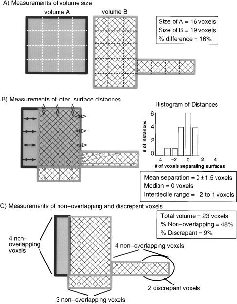
Illustration of four metrics used to compare segmented and warped lesion volumes. (A) Volume sizes were compared by computing absolute percent differences in the number of voxels included in two different segmented or warped lesion volumes. (B) Differences in the location of volumes were evaluated by measuring the relative Euclidean distances between the nearest voxels on two volume surfaces. The values computed across the surface voxels of two volumes formed a set of values that was analyzed using descriptive statistics. (C) Differences in location were also analyzed by computing the percentages of nonoverlapping and highly discrepant voxels across the total volume encompassed by a pair of segmented or warped lesion volumes.

Intersurface distances.

The demonstration of high agreement between measurements of volume size does not necessarily indicate high agreement about the shape and location of lesions; in the extreme case, two observers could segment identically sized, but completely nonoverlapping volumes. This issue has received little attention in previous attempts to segment lesions and quantify the reliability of the segmentation by different observers. However, the limitation of size comparisons is a critical issue for any study interested in evaluating the relationship between brain structure and brain function using the lesion method. For this reason, intra‐ and interobserver agreement in the segmentation and warping of lesion volumes was assessed through three additional measures that are more sensitive indicators of agreement about the location of segmented or warped lesion volumes [cf. Collins et al., 1995]: (1) differences in the location of the volume surfaces, (2) the percentage of voxels in two volumes that are nonoverlapping, and (3) the percentage of nonoverlapping voxels that are highly discrepant in location.

Differences in the location of volume surfaces were evaluated by measuring the relative Euclidean distance between the nearest voxels on two volume surfaces, using an automated algorithm [Frank et al., 1997] that implemented voxelwise 3D distance comparisons between the voxel locations in each surface tracing using a six‐neighbor rule [Russ, 1995] (Fig. 3b). Pairwise comparisons were made between segmented and between warped lesion volumes (e.g., the volume segmented by JF in a subject was compared to the volume segmented by HD in the same subject). The computed distances between the volume surfaces were thus zero where the surface voxels coincided, and nonzero integer values (indicating the number of voxels separating the two surfaces) elsewhere. Nonzero distance values were assigned positive values for where the surface voxel of the first volume extended beyond the nearest surface voxel of the second volume, and negative values where the surface voxel of the first volume extended less far than the nearest surface voxel in the second volume. The distance values that were computed across the surface voxels of the two volumes formed a set of values that was analyzed statistically for each intra‐ and interobserver volume comparison.

Nonoverlapping and discrepant voxels in total volumes.

As additional measures to evaluate differences in volume location, the percentages of nonoverlapping and highly discrepant voxels across the total volume encompassed by each segmented and warped lesion volume pair were computed (Fig. 3c). The percentage of nonoverlapping voxels in each volume pair was computed as the difference between the number of voxels in the total volume encompassed by both volumes vs. the number of voxels common to both volumes, divided by the number of voxels in the total volume.

Relatively small differences in the placement of lesion boundaries can lead to large cumulative effects over an entire volume. For instance, if a sphere with a 10‐voxel diameter were centered within an 11‐voxel diameter sphere, 25% of the total volume would be nonoverlapping. Such a high number can give the misleading impression that there is a substantial difference in the location of two volumes, even though the typical separation between the volume surfaces can be relatively small (e.g., for the two spheres the average separation is only 1 voxel). To give additional perspective upon the nonoverlap between two volumes, nonoverlapping voxels that were located more than 2 voxels from one or both volume surfaces were classified as discrepant voxels (the 2‐voxel criterion was based upon results from the inter‐surface analyses). Then, the percentage of discrepant voxels in the total volume was computed (number of discrepant voxels divided by the number of voxels in the total volume).

Creation and analysis of volumetric lesion overlap maps

Although the analysis of individual warped volumes provides information about variability in warping any single volume into a standard reference space, it provides little information about how this variability affects volumetric statistical maps that are based upon intersubject comparisons of the warped volumes. To assess this issue, six different volumetric lesion overlap maps were created by summing together each of the following sets of warped volumes: (1) the ten volumes transferred by JF from the consensus lesion, (2) the ten volumes transferred by HD from the consensus lesion, (3) the ten volumes directly transferred by JF, (4) the ten volumes directly transferred by HD, and (5) the ten volumes transferred using the automated AIR‐3 procedures (see Fig. 4). The lesion overlap volumes then were compared through pairwise subtractions. Voxels with identical values in both summed volumes (e.g., the voxel was included in seven of the nine individual warped volumes in both summed volumes) thus had zero values in the subtraction volume, and voxels with different values in the two summed volumes thus had values indicating the magnitude of the overlap count difference. The voxel values in each subtraction volume were then analyzed quantitatively through descriptive statistics such as mean value and standard deviation, and median value and interdecile range. The last measure was employed because normality tests (kurtosis, D'Agostino's D) indicated that the intersurface distance data were not normally distributed.

Figure 4.

Comparison of lesion overlap map created from the ten volumes warped by JF using MAP‐3 (A), the ten volumes warped by HD using MAP‐3 (B), and the ten volumes warped using AIR‐3 (C). As shown qualitatively through the surface renderings and coronal sections, the lesion overlap maps are very similar (red = site of maximal lesion overlap, blue = site of minimal lesion overlap). This conclusion is supported quantitatively by pairwise subtractions of the lesion overlap volumes; as shown in the histograms (D), the typical difference in lesion overlap count across is zero, with an interdecile range of ± 1.

RESULTS

Variability in lesion segmentation

Volume size.

Table I summarizes the size of the volumes segmented by each observer in each of the ten subjects. On average, the intraobserver absolute difference in volume size was 17 ± 12% in JF, and 12 ± 8% in HD. The interobserver absolute difference in volume size was comparable, at 18 ± 16%. Interrater and intrarater reliability can be assessed by intraclass correlation values. Overall, the intraclass correlation coefficients were high, indicating substantial agreement between observers about the size of the segmented volumes: r(1,2) = .86 and .95 for JF and HD, respectively, and r(1,2) = .88 for JF vs. HD. The values for the interobserver comparisons for two subjects (1811fl and 071gmg) are quite high; the causes for disagreement will be discussed later, and are illustrated in Figure 5.

Table I.

Differences in segmented volume sizes across observer comparisons*

Subject	No. voxels inside trace boundary				Absolute difference (%)
	JF		HD		Intra		Inter
	A	B	A	B	JF	HD
0468jg	23700	25152	23409	25366	5	8	1
0675es	9961	9429	10110	9458	5	7	1
0716mg	13068	14218	20798	20581	8	1	46
1039ba	19063	29358	24318	21114	43	14	24
1198rs	13884	12207	11591	15402	13	28	18
1492tk	18557	13831	18772	22256	29	17	1
1496jb*	14122	15941	16244	17785	12	9	14
1662sc	13106	15446	15199	16702	16	9	15
1726ro	27133	28800	30368	27626	6	9	11
1811fl	5974	4547	3788	4691	27	21	45
Mean ± SD	17 ± 12	12 ± 8	18 ± 16

^*Voxel sizes for 1496jb were 0.94 × .94 × 3.00 mm, and .94 × .94 × 1.5 mm for all other subjects.

Figure 5.

Illustration of intra‐ and interobserver variability in the segmentation of lesion boundaries. The lesion contours traced by two different observers are shown for two subjects [left panel shows a single coronal section from 0716 mg (one of the “discrepant” cases), right panel shows a single coronal section from 1492tk]. The top and middle rows illustrate intraobserver comparisons (top row: compare red line showing first trace by JF to blue line showing second trace by JF; middle row: compare red line showing first trace by HD to blue line showing second trace by HD). The bottom row illustrates interobserver comparisons (compare pink line showing first trace by JF to blue line showing first trace by HD). Sources of variability include minor discrepancies associated with interpreting the transition from lesioned to nonlesioned tissue and manually moving a cursor (A), and larger discrepancies caused by drawing along an imagined gyral edge (B), deciding whether a voxel represents damaged tissue vs. normal intersulcal space (C), or whether a voxel represents damaged tissue vs. an obliquely cut gyrus (D).

Intersurface distances.

Table II summarizes the statistics for the distances between segmented lesion volume surfaces, for both intra‐ and interobserver comparisons of the segmented volumes in each subject. Across all subjects, the mean of the distances between intra‐ and interobserver comparisons of volume surfaces was zero. Because the surface distances were measured in relative terms (with negative values where the first surface extended less far than the second surface, and positive values where the first surface extended further than the second surface), the mean value of zero does not indicate that the surfaces were perfectly aligned. Rather, it indicates that the observers did not systematically differ in the size of the segmented volumes (e.g., one observer did not always segment out a larger volume).

Table II.

Mean and median statistics for distances between segmented volume surfaces

Subject	Mean			SD			Median			10th %ile			90th %ile
	Intra		Inter	Intra		Inter	Intra		Inter	Intra		Inter	Intra		Inter
	JF	HD		JF	HD		JF	HD		JF	HD		JF	HD
0468jg	1	0	1	4	1	5	0	0	0	−2	−1	−2	9	1	10
0675es	0	0	0	1	1	1	0	0	0	−2	−1	−1	2	1	1
0716mg	−1	0	−1	2	1	2	0	0	−1	−3	−1	−4	2	1	1
1039ba	−4	−3	0	7	7	1	−1	0	0	−16	−17	−2	1	1	1
1198rs	0	1	0	1	1	2	0	1	0	−1	−1	−2	2	3	1
1492tk	3	1	0	6	3	1	1	0	0	−1	−1	−2	11	5	1
1496jb	0	0	−1	1	1	1	−1	0	−1	−2	−1	−2	1	2	1
1662sc	0	0	−1	2	1	3	0	0	−1	−2	−1	−3	1	1	1
1726ro	0	0	0	1	1	2	0	0	0	−2	−1	−2	1	1	2
1811fl	1	0	1	1	1	1	1	0	1	−1	−1	−1	2	2	2
Mean	0	0	0	3	2	2	0	0	0	−3	−3	−2	3	2	2

The standard deviations of the surface distances from the mean are an indicator of how well the two surfaces are aligned. Across subjects, the average intraobserver standard deviation was ± 3 (JF) and ± 2 (HD) voxels, and the average interobserver standard deviation was ± 2 voxels. The intersurface distances values were not distributed normally, as demonstrated by the presence of significant leptokurtosis (p < 0.05 for n > = 2000) in nine of the ten surface distance datasets comparing the first and second segmentation of the lesions by HD, nine of ten for JF, and nine of ten comparing the first segmentation of HD to the first segmentation of JF. As a further assessement, we also calculated D'agostino's D, a more sensitive measure of normality [Zar, 1974], for these datasets, and in all cases, the null hypothesis of normal distribution was rejected (observed values of D 0. 2016 − 0. 2685, n 1695–8516, lower critical value for n = 2000 and p = 0.05, 0. 2807). Thus, standard deviation values overestimate the degree of variability in the location of the volume surfaces. This fact can be appreciated by considering the interdecile (10–90%) range of distance values. The typical interdecile range was similar to the standard deviation values [an average of ± 3 voxels (JF) and −3 to 2 voxels (HD) for intraobserver comparisons, and ± 2 for interobserver comparisons]. If the distribution were normal, an interdecile range of ± 4 voxels would be expected on the basis of the observed standard deviation values.

The difference between the expected and the actual interdecile range reflects the fact that much of the variance between the location of volume surfaces is caused by large differences over relatively small portions of the volume surfaces. This is illustrated in Figure 5, where one observer extended the volume boundary to include a gyrus that was considered normal by the other observer; the two observers substantially agreed about the location of lesioned tissue elsewhere. In practice, the intra‐ and interobserver agreement about the location of the segmented volume surfaces was high: for any two compared volumes, over 80% of the volume surfaces were located within just 2–3 voxels of each other (2–4.5 mm in the present study).

Nonoverlapping and discrepant voxels.

Table III summarizes the percentages of nonoverlapping voxels for the intra‐ and interobserver comparison of segmented volumes, in each of the ten subjects. On average, for intraobserver comparisons of lesion volumes, 36 ±7% (JF) and 26 ± 6% (HD) of the voxels in the total volume were nonoverlapping. For interobserver comparisons, 33 ± 7% of the voxels in the total volume were nonoverlapping.

Table III.

Percentages of nonoverlapping and discrepant voxels across segmented volumes

Subject	Total volume size*			Nonoverlapping (%)			Discrepant (%)
	Intra		Inter	Intra		Inter	Intra		Inter
	JF	HD		JF	HD		JF	HD
0468jg	28473	27377	28999	28	22	31	10	1	9
0675es	11566	10971	10956	35	22	25	3	2	2
0716mg	17349	23243	21930	43	22	47	9	1	10
1039ba	30438	26692	22731	41	30	23	23	12	3
1198rs	15305	16203	17352	30	33	31	3	4	4
1492tk	21497	24701	24033	49	34	30	24	10	2
1496jb	18247	19019	19267	35	21	34	0	1	5
1662sc	17077	18241	18324	33	25	37	4	1	7
1726ro	32594	32599	32810	28	22	33	2	3	4
1811fl	6391	5105	6643	35	34	39	5	1	4
Mean ± SD	36 ± 7	26 ± 6	33 ± 7	8 ± 9	4 ± 4	5 ± 3

^*Total volume size refers to the size of all voxels included in either of the compared volumes (e.g, either of the volumes segmented by JF for the JF intra comparison). The values are thus larger than the size of the individual volumes listed in Table I.

As noted above, for both intra‐ and interobserver comparisons of volume surfaces, the distances separating the surfaces had a small interdecile range (typically, the distance values in the middle 80% of the distribution fell within ± 2 voxels). As would be expected on the basis of this finding, for both intra‐ and interobserver comparisons, a relatively small fraction of the total volume consisted of discrepant voxels—nonoverlapping voxels more than 2 voxels away from one or both of the volume surfaces. Specifically, for intraobserver comparisons, 8 ± 9% (JF) and 4 ± 4% (HD) of the voxels were discrepant, and for interobserver comparisons 5 ± 3% of the voxels were discrepant.

Variability in MAP‐3 warped volumes

Volume size.

Table IV summarizes, for each subject, the size of the MAP‐3 volumes manually warped by each observer from the consensus lesion volume. On average, the interobserver difference in volume size was 15 ± 8%. Evaluation of the interrater reliability indicated that there was a high agreement on volume size between observers, based upon the intraclass correlation coefficient [r(1,2) = .90]. Similar results were obtained when the MAP‐3 manual warping was based upon a direct transfer of the lesion to the reference brain [the mean interobserver difference in volume size was 14 ± 11%, and the intraclass correlation coefficient was r(1,2) = .95].

Table IV.

Differences in MAP‐3 volume sizes for consensus transfers

Subject	No. voxels inside trace boundary			Absolute difference (%)
	JF	HD	AIR	JF vs. HD	AIR vs. JF	AIR vs. HD
0468jg	21313	28916	28129	30	28	3
0675es	11852	13861	13568	16	14	2
0716mg	22071	20266	24438	9	10	19
1039ba	20463	23410	24080	13	16	3
1198rs	16190	18676	16967	14	5	10
1492tk	23621	26233	18773	10	23	33
1496jb	26630	27366	28564	3	7	4
1662sc	17120	21805	24237	24	34	11
1726ro	29863	32127	28679	7	4	11
1811fl	6021	4798	7752	23	25	47
Mean ± SD		15 ± 8	17 ± 11	14 ± 15

Results from the automated AIR‐3 based warping of the consensus lesions are also summarized in Table IV. Comparison of the AIR‐3 segmented volumes to the manually warped volumes indicates that the typical agreement between human observers is comparable to the typical agreement between manual and automated warping methods. The mean MAP‐3 vs. AIR‐3 difference in size was 17 ± 11% (JF vs. AIR‐3) and 14 ± 15% (HD vs. AIR‐3), and the intraclass correlation coefficients were high [r(1,2) = .85 (JF vs. AIR‐3) and .91 (HD vs. AIR‐3)]. Despite generally good performance relative to manual methods, the AIR‐3 algorithm produced poorer results for some subjects: the largest differences in volume size were all found in comparisons of AIR‐3 vs. MAP‐3 warped volumes (e.g., see subjects 1811fl and 1492tk, and Fig. 7).

Figure 7.

Illustration of intraobserver variability in the transfer of lesion boundaries using MAP‐3. Comparisons between the transfer volumes for JF (shown in red on the coronal sections and leftmost 3D rendered brains) and HD (shown in blue on the coronal sections and rightmost 3D rendered brains) are shown for three subjects (top: 0468jg, middle: 0716 mg, bottom: 1198rs). Areas of overlap are shown in yellow. Most of the differences were minor (e.g., compare position of boundary edges in the second coronal section in each row). Larger discrepancies represent factors such as deciding whether the lesion extends into a new gyrus (e.g., compare the red vs. blue boundaries in the third section of the bottom row). The overall similarity in the transfer volumes is well illustrated by the similarities in location and extent on the 3D rendered brains.

Intersurface distances.

Table V summarizes, for each subject, the statistics for the distances between the MAP‐3 manually warped volume surfaces transferred by each observer. Across subjects, the mean distance between volume surfaces warped by the two observers was zero. This indicates that the observers did not systematically differ in their localization of the segmented volumes (e.g., one observer did not always create a larger warped volume or extend further into the white matter).

Table V.

Mean distances and interdecile ranges between MAP‐3 volume surfaces for consensus transfers

Subject	JF vs. HD (Mean ± SD)	Interdecile range	AIR vs. JF (Mean ± SD)	Range	AIR vs. HD (Mean ± SD)	Range
0468jg	−1 ± 2	−4–1	1 ± 2	−2–3	0 ± 2	−3–2
0675es	0 ± 2	−2–2	0 ± 2	−2–2	0 ± 2	−3–3
0716mg	0 ± 2	−2–3	0 ± 3	−3–4	0 ± 2	−2–3
1039ba	0 ± 2	−3–2	1 ± 3	−2–2	0 ± 2	−3–2
1198rs	0 ± 1	−2–1	0 ± 2	−4–2	0 ± 2	−3–1
1492tk	0 ± 2	−2–2	−1 ± 2	−4–2	−1 ± 2	−4–1
1496jb	0 ± 2	−2–2	0 ± 3	−4–5	0 ± 2	−3–3
1662sc	−1 ± 2	−3–1	1 ± 2	−2–4	0 ± 1	−1–2
1726ro	0 ± 2	−2–2	−1 ± 3	−5–3	−1 ± 3	−5–3
1811fl	0 ± 2	−1–2	0 ± 2	−2–2	1 ± 1	−1–3
Mean	0 ± 2	−2–2	0 ± 2	−3–3	0 ± 2	−3–2

The standard deviations of the surface distances were relatively large: across subjects, the average standard deviation was ± 2 voxels. However, as was found for the comparisons of segmented volumes, the distance values were not normally distributed. D'agostino's D test rejected the null hypothesis of normal distribution for 9/10 surface distance datasets generated by comparing the AIR‐3 transfer to HD's MAP‐3 transfer (D observed 0. 2264–0. 2814, n 2411–7583, lower critical D for n = 2000 and p = 0.05 is 0. 2807), and 10/10 surface distance datasets comparing AIR‐3 to JF, or HD to JF (D observed 0. 2497–0. 2777, all significant at p < 0.05) [Zar, 1974]. The values in the middle 80% of the distribution had an interdecile range of ± 2 voxels. The fact that the interdecile range is comparable to the standard deviation reflects the fact that much of the variance between the location of the volume surfaces is caused by large differences over relatively small portions of the volume surfaces (e.g., see Fig. 6).

Figure 6.

Illustration of a discrepancy in the transfer of lesion boundaries using MAP‐3 vs. AIR‐3. (A) 3D‐reconstructed brain of subject 1726ro after it was warped to the template brain. The blue area shows the lesion to be transferred to the normal brain. (B) The MAP‐3 warps by HD and JF are shown in green and red, with the area of overlap indicated in yellow. The warp produced by AIR‐3 is shown by the blue lines. The agreement between human observers is very good, but the agreement between methods (MAP‐3 vs. AIR‐3) is poor because the basal ganglia are damaged but AIR‐3 does not include them in the lesion.

As expected, slightly more variability was found for the direct MAP‐3 transfers. The mean of the distances between volume surfaces was zero, and the mean standard deviation of the distance values was ± 3 voxels. Once again, the distance values were normally distributed: the mean interdecile range of the distance values was −3 to 3 voxels, which is comparable to the mean standard deviation.

Table V also summarizes, for each subject, the statistics for comparisons between MAP‐3 and AIR‐3 warped volumes. On average, the agreement between manually‐based MAP‐3 warps and the automated AIR‐3 based warps was slightly less than the agreement between two human observers using the MAP‐3 technique. The mean of the distances between the volume surfaces was zero, the mean standard deviation of the distance values was ± 2 voxels, and the interdecile range was within ± 3 voxels. Despite generally good performance relative to manual methods, the AIR‐3 algorithm did produce poorer results in some subjects: the greatest variance in distance values were all found in comparisons of AIR‐3 vs. MAP‐3 warped volumes (e.g., see subjects 1726ro and 1496jb; Fig. 7).

Nonoverlapping and discrepant voxels.

Table VI summarizes, for each subject, the percentage of nonoverlapping voxels between the MAP‐3 warped volumes transferred by each observer. On average, 41 ± 6% of the voxels in the total volume were nonoverlapping. A small fraction (6 ± 2%) of the total volume consisted of discrepant voxels—voxels further than 2 voxels away from one or both of the volume surfaces. For the direct transfers, 49 ± 10 of the voxels were nonoverlapping, and 12 ± 9% of the total volume consisted of discrepant voxels.

Table VI.

Nonoverlapping and discrepant voxels across MAP‐3 volumes for consensus transfers*

Subject	JF vs. HD			AIR vs. JF			AIR vs. HD
	Total	Nonoverlap	Discrepant	Total	Nonoverlap	Discrepant	Total	Nonoverlap	Discrepant
0468jg	32102	44%	9%	30740	39%	5%	34769	36%	6%
0675es	15945	45%	7%	16288	44%	4%	18466	51%	10%
0716mg	25992	37%	5%	30010	45%	13%	27832	39%	5%
1039ba	28578	46%	7%	30498	54%	14%	30881	46%	7%
1198rs	20497	30%	1%	20041	35%	4%	20896	29%	3%
1492tk	30173	35%	5%	27389	45%	12%	27969	39%	9%
1496jb	33757	40%	7%	37393	52%	20%	35651	43%	10%
1662sc	24710	42%	9%	27222	48%	15%	27675	34%	2%
1726ro	37647	35%	4%	40710	56%	19%	41080	52%	19%
1811fl	7263	51%	4%	9076	48%	5%	8388	50%	5%
Mean ± SD	41 ± 6%	6 ± 2%	47 ± 7%	11 ± 6%	42 ± 8%	8 ± 5%

^*Total volume size refers to the size of all voxels included in either of the compared volumes (e.g, in either the volumes transferred by JF or by HD in the “JF vs. HD” comparison). The values are thus larger than the size of the individual transfer volumes listed in Table IV.

Table VI also summarizes, for each subject, the statistics for comparisons between MAP‐3 and AIR‐3 warped volumes. On average, the agreement between warps produced using the two procedures was slightly less than the agreement between two human observers using the MAP‐3 technique. The mean percentage of nonoverlapping voxels was 42% (JF vs. AIR‐3) and 42% (HD vs. AIR‐3), and the percentage of discrepant voxels was 11% (JF vs. AIR‐3) and 8% (HD vs. AIR‐3). Despite generally good performance relative to manual methods, the AIR‐3 algorithm did produce poorer results in some subjects: the largest percentages of nonoverlapping and discrepant voxels were all found in comparisons of AIR‐3 vs. MAP‐3 warped volumes (e.g., see subjects 1496jb, 1726ro).

Variability in volumetric lesion overlap maps created from warped volumes

Comparisons between the MAP‐3 volumes were also conducted by summing together the warped volumes to create a lesion overlap map, and then conducting pairwise subtractions between different summed volumes to isolate differences in the lesion overlap values in the two summed volumes. A comparison of the lesion overlap volumes created from sets of MAP‐3 warped volumes that were manually transferred by two different observers revealed a mean difference of zero and a standard deviation of ± 1; this indicates that, on average, the lesion overlap values in the two summed volumes were identical, though there were relatively small differences between the volumes. As found in previous analyses, the values were not normally distributed: the median value was zero, and the interdecile range was ± 1. Thus, over 80% of the voxel values in the lesion overlap maps were identical or nearly identical (differing only by a count of one subject). For the direct transfers, the mean difference was −3, the standard deviation was ± 1, the median was zero, and the interdecile range was ± 1. The similarities between the two volumes can also be appreciated through a qualitative inspection of the images (see Fig. 4). The overlap maps show a region of maximal overlap that involves the same cortical and subcortical neuroanatomical structures.

A comparison of the lesion overlap volume created from the AIR‐3 warps of the consensus lesion to the lesion overlap volumes created using the MAP‐3 procedure revealed slightly more variability, though the maps were still very similar. For the JF vs. AIR‐3 overlap map comparison, the mean difference was 0 ± 1 voxel SD, and the median was zero with an interdecile range of −2 to 1. For the HD vs. AIR‐3 overlap map comparison, the mean difference was 0 ± 1 voxel SD, and the median was zero with an interdecile range of 1–2. Visual inspection of the differences between the overlap volumes reveals a high degree of similarity to the maps created from the MAP‐3 procedure at the cortical surface. More variability is observed in the subcortical extent of the maximal overlap, particularly in the relationship between the lesion overlap and the basal ganglia.

DISCUSSION

The results of the lesion segmentation and warping comparisons permit the following conclusions. First, the methods employed in this paper for the manual segmentation and warping of lesion volumes produce reliable results. Both intra‐ and interobserver comparisons indicate that the agreement between observers is high, and the variability in the placement of lesion boundaries is well below the anatomical scale at which conclusions are usually drawn based upon evidence obtained with these procedures. The typical purpose of lesion segmentation and warping is to define the location of brain damage. The measurements of intersurfaces distances indicated that the separation between two segmented or warped volume surfaces had a variance of about ± 2 voxels. This is high estimate of the variance, because, in every case, the distance values were not distributed normally; in practice, approximately 80% of the surface voxels were separated by no more than 2 voxels (∼ 2 mm³ for the images in this study). In general, less than 10% of the total volume encompassed by any two segmented or warped volumes consisted of discrepant voxels beyond the typical ± 2 voxel interdecile range.

Based upon these estimates of variance in location, lesion segmentation and warping methods can produce results that rival other functional brain mapping techniques. In functional neuroimaging studies, intersubject comparisons are often based upon data smoothed to a resolution of 6–12 mm, and the locations of peak activation can easily vary by 6–10 mm across subjects. More importantly, the variability observed between comparisons is well below the level of anatomical detail usually sought from the lesion method. For instance, in a previous report using the MAP‐3 technique, the focus was upon neuroanatomical regions separated by more than two centimeters [Damasio et al., 1996; Tranel et al., 1997]. Thus, although the boundaries of segmented and warped lesions cannot be determined with complete agreement between observers and techniques, the variance in the lesion boundaries is unlikely to affect neuroanatomical claims that are based upon the attributions of lesions to structural areas whose size is on the order of a centimeter or more.

A second conclusion is that the intra‐ and interobserver differences were of comparable magnitude. This finding is important for two reasons. First, it indicates that much of the difficulty involved in lesion segmentation and warping arises from subjective decisions that do not systematically differ between observers. For instance, observers do not appear to choose different intensity thresholds values for lesioned tissue that they use consistently across subjects—if this were the case, the intraobserver differences should be much smaller than the interobserver differences. Second, significant amounts of prior experience does not appear to lower the intraobserver variability dramatically—only slightly more variability was observed for comparisons involving volumes that were segmented and warped by the observer with hours vs. years of experience. This result suggests that naive users can become proficient with the MAP‐3 technique relatively quickly, provided that they start with a good knowledge of macroscopic neuroanatomy.

A third conclusion is that the statistical volumes created from sets of warped volumes transferred by different observers and techniques were very similar. Such overlap maps are the basis upon which group comparisons and structure‐function correlations can be made using the MAP‐3 technique [e.g., see Damasio et al., 1996; Frank et al., 1997; Tranel et al., 1997]. Thus, it is critical that the contours of these maps are relatively constant across observers, and that they are resistant to variability at the level of the individual warped volumes. This was shown to be the case through pairwise comparisons of the lesion overlap volumes. Figure 4 highlights the fact that the statistical maps created from different sets of warped lesion volumes are very similar, despite use of a manual warping technique that forces each observer to make a large number of subjective decisions, and an automated technique that is susceptible to lesion‐induced distortions in neuroanatomy.

A fourth conclusion is that an automated technique for lesion warping based upon the AIR‐3 registration algorithm can produce results that rival a manual technique in most subjects. This fact can be appreciated by noting that the variability found in comparisons of AIR‐3 vs. MAP‐3 warped volumes was generally similar to the variability found in interobserver comparisons of MAP‐3 volumes. It is important to note, however, that in some cases the AIR‐3 method produced results that were clearly different from the warped volumes created by human observers. The underlying causes for this occasionally poorer performance and the implications for the use of AIR‐3 as an automated warping method are discussed below. It is also important to note that many laboratories use simpler automated warping procedures (e.g., a 9‐parameter affine transformation). Simpler procedures will almost certainly produce results that are inferior to the nonlinear AIR algorithm and that are even further from human performance. For instance, Collins et al. [1995] showed that a linear approach resulted in poor superposition of the ventricles across subjects, and Woods et al. [1998a, b] demonstrated progressively better registration of macroscopic landmarks by AIR as the polynomial order of the spatial transformation model was increased. The acceptability of the amount of variance produced by a given method will depend upon the objective of each study that employs lesion segmentation and warping procedures. For instance, if the goal is to localize a site of maximal overlap with the greatest possible precision, then the MAP‐3 manual warping method should be employed, although even this technique will have limits (e.g., it will not support neuroanatomical claims at the scale of millimeters). If the goal is to localize the site of maximal overlap to a particular gyrus, then manual and automated linear and nonlinear methods may all produce acceptable results.

Sources of variability in lesion segmentation and warping

Inspection of the segmented and warped volumes created by different observers and methods provides important information about the underlying causes of variability within and between observers. Most of the small disagreements (< 2 voxels) appear to arise when there is consensus about the presence of lesioned tissue, but disagreement about the exact voxel intensity associated with the transition from lesioned to nonlesioned tissue (in the case of lesion segmentation) or the extent to which the warped volume should extend into a particular gyrus or into the white matter. Potentially, these sources of disagreement could be minimized by the incorporation of objective means for tissue classification and the use of more sophisticated warping procedures. On the other hand, these inconsistencies may well represent reality—pathological changes, even when examined under the microscope, do not provide a clear cleavage between damaged and healthy tissue, but rather an area of transition. Other factors appear to give rise to larger but less frequent disagreement. The sources of these disagreements often arise out of uncertainty about the presence or absence of lesioned tissue, and they will be harder to eliminate. Any attempt to develop automated procedures for lesion segmentation and warping will need to develop new approaches (e.g., knowledge‐based decision‐making strategies, or the examination of multimodal data) to deal with these sources of ambiguity. Examples and further discussion of the sources of variability in lesion segmentation and warping are provided below.

Variability in lesion segmentation.

For both intra‐ and interobserver comparisons of segmented volume surfaces, the interdecile range of distances between the surfaces was typically ± 2 voxels. As illustrated in Fig. 5a, these small differences in the delineation of lesion boundaries reflect, in large part, general agreement about the presence of lesioned tissue, but (1) disagreement about the exact voxel intensity value associated with the transition from lesioned to nonlesioned tissue, and (2) the variability inherent in manually tracing along an agreed‐upon boundary.

Other factors give rise to larger (> 2 voxel), but less frequent, separations between the volume surfaces. One source of disagreement is the destruction of surface landmarks, so that the lateral extent of a lesion must be extrapolated from nearby intact surface structures (Fig. 5b). This type of disagreement is trivial, in the sense that although the boundaries may be variable, there is agreement that the entire neuroanatomical region is affected. A second source of disagreement arises when the voxel intensity values of the lesion overlap with the expected values in similarly located normal tissue. For instance, it can be difficult to distinguish between lesioned tissue and intersulcal fluid (Fig. 5c), or between lesioned tissue and the transverse edge of a gyrus (Fig. 5d). Disagreements of this type are more serious, because they reflect uncertainty about whether a particular neuroanatomical region is or is not damaged. However, neither of these factors is a major source of variability: on average, for any two compared volumes, fewer than 6% of the nonoverlapping voxels were more than 2 voxels away from one or both volume surfaces.

Variability in MAP‐3 warped volumes.

Multiple factors also appear to give rise to interobserver differences in the MAP‐3 transfer of lesion volumes (see Fig. 6). When the variability in lesion segmentation is removed by first defining a consensus lesion volume, the separations between the warped volume surfaces fall within a narrow interdecile range of ± 2 voxels. These small differences reflect, in large part, general agreement about the correspondence between damaged neuroanatomical structures in the lesioned brain and intact structures in the normal reference brain, but disagreement about the precise warping (e.g., how far the warped volume should extend into white matter). Larger (> 2 voxel), but less frequent, differences between volume surfaces appear to arise largely from uncertainty about correspondences between neuroanatomical structures. For instance, it may be difficult to determine whether the lesion volume is limited to the inferior frontal gyrus, or whether portions of the orbital frontal gyrus are also damaged.

The variability found in comparisons of MAP‐3 vs. AIR‐3 warped volumes was generally similar to the variability found in interobserver comparisons of MAP‐3 volumes. However, the automated procedure is adversely affected by large distortions of CSF‐containing spaces, because of overlap in the pixel intensity values for lesioned tissue and CSF. The lack of a clear boundary between lesioned and nonlesioned tissue disrupts the overall warping of the lesioned brain into the space of the reference brain, resulting in parameter errors for the warp that are propagated through to the transfer of the consensus lesion volume into the space of the reference brain. Human observers are better able to compensate for such distortions in the normal relationships between tissues. An example of these points are illustrated in Figure 7; in which the agreement between warped volumes produced by different human observers is very good, but the agreement between methods (AIR‐3 vs. MAP‐3) is very poor.

Overall, our findings indicate the AIR‐3 method has two uses that are most appropriate. First, it could be used to support a semiautomated method that combines elements from both the AIR‐3 and the MAP‐3 methods. AIR‐3 could be used to accomplish steps 1 and 2 of the MAP‐3 method, which involves finding a similar slice orientation and thickness for the lesioned and reference brains. These steps are the most time‐consuming aspects of the MAP‐3 method. The lesion contours could then be directly transferred onto the resliced reference brain using a manual tracing technique. In an experienced observer, this tracing does not require significantly more time than segmenting a lesion for automated transfer to a reference brain using AIR‐3, and thus the time to implement this type of semiautomated approach should rival the time required to implement a manual segmentation followed by fully automated AIR‐3 based‐warping.

Second, the AIR‐3 method may be sufficient when the objective is to draw general conclusions from statistical volumes created from a relatively large number of individually warped volumes (which would serve to minimize discrepant contributions from a small number of subjects). As noted above, in the present study, the lesion overlap volume created from the AIR‐3 warped volumes was found to be very similar to the lesion overlap volumes created from MAP‐3 warped volumes (see Fig. 4), with an overall variability that is below the level of detail usually sought from the lesion method. However, individual warps created by AIR‐3 should be screened by a human observer to rule out large discrepancies caused by distortions in the normal relationships between anatomical structures (e.g., because of enlarged ventricles). Furthermore, the AIR‐3 method may not be sufficient for investigators interested in examining cases in which individuals are discrepant with the results from the overlap maps (e.g., accounting for a subject with a lesion in the maximal zone of lesion overlap, but with no corresponding behavioral deficit); in this case, it is desirable to begin with the best possible warping of lesions into a reference space.

CONCLUSIONS

These results demonstrate the utility of manual segmentation and MAP‐3 warping techniques for detailed neuroanatomical investigations in brain‐damaged subjects. The variability in the implementation of these procedures is well below the resolution of the neuroanatomical conclusions, which are usually drawn from these procedures. Furthermore, these techniques can be learned easily (< 10 hr for each procedure, provided that there is a good knowledge about normal anatomy at the macroscopic level), as demonstrated by the relatively small differences seen between the intraobserver variability for the experienced observer, vs. the intraobserver variability for the inexperienced observer.

Although there is not a “gold standard” by which to judge segmentation and warping procedures, this study does provide benchmark performance levels for human observers. Comparison of the manual MAP‐3 technique to an automated technique based upon the AIR‐3 image registration algorithm revealed that the AIR‐3 approach produced favorable levels of performance in most, but not all, subjects. Our results also illustrate the difficulties inherent in the segmentation and warping of lesion volumes that warrant particular attention in the development of automated segmentation and improved warping procedures. Novel automated techniques could be evaluated using the same analysis techniques and dataset, to determine whether the variability across manual and automated techniques is within the same range as that found across human observers.

REFERENCES

- Bedell BJ, Narayana PA, Wolinsky JS. 1997. A dual approach for minimizing false lesion classifications on magnetic resonance images. Magn Reson Med 37: 94–102. [DOI] [PubMed] [Google Scholar]
- Bendszus M, Urbach H, Meyer B, Schultheiss R, Solymosi L. 1997. Improved CT diagnosis of acute middle cerebral artery territory infarcts with density‐difference analysis. Neuroradiology 39: 127–131. [DOI] [PubMed] [Google Scholar]
- Christensen GE, Joshi SC, Miller MI. 1997. Volumetric transformation of brain anatomy. IEEE Trans Med Imaging 16: 864–877. [DOI] [PubMed] [Google Scholar]
- Collins DL, Holmes CJ, Peters TM, Evans AE. 1995. Automatic 3‐D model‐based neuroanatomical segmentation. Hum Brain Mapp 3: 190–208. [Google Scholar]
- Damasio H, Damasio AR. 1980. The anatomical basis of conduction aphasia. Brain 103: 337–350. [DOI] [PubMed] [Google Scholar]
- Damasio H, Frank R. 1992. Three‐dimensional in vivo mapping of brain lesions in humans. Arch Neurol 49: 137–143. [DOI] [PubMed] [Google Scholar]
- Damasio H, Grabowksi TJ, Tranel D, Hichwa RD, Damasio AR. 1996. A neural basis for lexical retrieval. Nature 380: 499–505. [DOI] [PubMed] [Google Scholar]
- Dastidar P, Heinonen T, Vahvelainent T, Elovaara I, Eskola H. 1999. Computerised volumetric analysis of lesions in multiple sclerosis using new semi‐automatic segmentation software. Med Biol Eng Comput 37: 104–107. [DOI] [PubMed] [Google Scholar]
- Filippi M, Horsfield MA, Bressi S, Martinelli V, Baratti C, Reganati P, Campi A, Miller DH, Comi G. 1995. Intra‐ and interobserver agreement of brain MRI lesion volume measurements in multiple sclerosis: A comparison of techniques. Brain 118: 1593–1600. [DOI] [PubMed] [Google Scholar]
- Fox PT, Perlmutter JS, Raichle ME. 1985. A stereotactic method of anatomical localization for positron emission tomography. J Comput Assist Tomogr 9: 141–153. [DOI] [PubMed] [Google Scholar]
- Fox PT, Mintun MA, Reiman EM, Raichle ME. 1988. Enhanced detection of focal brain responses using intersubject averaging and change‐distribution analysis of subtracted PET images. J Cereb Blood Flow Metab 8: 642–653. [DOI] [PubMed] [Google Scholar]
- Frank RJ, Damasio H, Grabowski TJ. 1997. Brainvox: An interactive, multi‐modal, visualization and analysis system for neuroanatomical imaging. Neuroimage 5: 13–30. [DOI] [PubMed] [Google Scholar]
- Friston KJ, Frith CD, Liddle PF, Frackowiak RSJ. 1991. Plastic Transformation of PET Images. J Comput Assist Tomogr 15: 634–639. [DOI] [PubMed] [Google Scholar]
- Gibbs P, Buckley D, Blackband S, Horsman A. 1996. Tumour volume determination from MR images by morphological segmentation. Phys Med Biol 41: 2437–2446. [DOI] [PubMed] [Google Scholar]
- Haller JW, Christensen GE, Joshi SC, Newcomer JW, Miller MI, Csernansky JG, Vannier MW. 1996. Hippocampal MR imaging morphometry by means of general pattern matching. Radiology 199: 787–791. [DOI] [PubMed] [Google Scholar]
- Kunesch E, Binkofski F, Steinmetz H, Freund HJ. 1995. The pattern of motor deficits in relation to the site of stroke lesions. Eur Neurol 35: 20–26. [DOI] [PubMed] [Google Scholar]
- Naeser MA, Hayward RW. 1978. Lesion localization in aphasia with cranial computed tomography and the Boston Diagnostic Aphasia Exam. Neurology 28: 545–551. [DOI] [PubMed] [Google Scholar]
- Russ C. 1995. The image processing handbook, 2nd Edition CRC Press: Boca Raton, FL. [Google Scholar]
- Schormann T, Zilles K. 1998. Three‐dimensional linear and non‐linear transformations: An integration of light microscopical and MRI data. Human Brain Mapp 6: 339–347. [DOI] [PMC free article] [PubMed] [Google Scholar]
- Soltanian‐Zadeh H, Peck DJ, Windham JP, Mikkelsen T. 1998. Brain tumor segmentation and characterization by pattern analysis of multispectral NMR images. NMR Biomed 11: 201–208. [DOI] [PubMed] [Google Scholar]
- Sorlie C, Bertrand O, Yvert B, Froment J, Pernier J. 1997. Matching of digitised brain atlas to magnetic resonance images. Med Biol Eng Comput 35: 239–245. [DOI] [PubMed] [Google Scholar]
- Talairach J, Tournoux P. 1988. Co‐planar stereotaxic atlas of the human brain (translated by Mark Rayport). New York: Thieme Medical Publishers, Inc. [Google Scholar]
- Tranel D, Damasio H, Damasio AR. 1997. A neural basis for the retrieval of conceptual knowledge. Neuropsychologia 35: 1319–1327. [DOI] [PubMed] [Google Scholar]
- Woods D, Knight R, Scabina D. 1993. Anatomical substrates of auditory selective attention: Behavioral and electrophysiological effects of posterior association cortex lesions. Brain Res Cogn Brain Res 1: 227–240. [DOI] [PubMed] [Google Scholar]
- Woods RP, Grafton ST, Holmes CJ, Cherry SR, Mazziotta JC. 1998a. Automated image registration: I. General methods and intrasubject, intramodality validation. J Comput Assist Tomogr 22: 139–152. [DOI] [PubMed] [Google Scholar]
- Woods RP, Grafton ST, Watson JD, Sicotte NL, Mazziotta JC. 1998b. Automated image registration: II. Intersubject validation of linear and nonlinear models. J Comput Assist Tomogr 22: 153–165. [DOI] [PubMed] [Google Scholar]
- Zar JH. 1974. Biostatistical analysis. Englewood Cliffs, NJ: Prentice‐Hall, Inc. [Google Scholar]