Implementation and application of a brain template for multiple volumes of interest

Abstract

We present a region template and a protocol for transforming that template to define anatomical volumes of interest (VOIs) in the human brain without operator intervention, based on software contained in the SPM99 package (Statistical Parametric Mapping, Wellcome Department of Cognitive Neurology, London, UK). We used an MRI of a reference brain to create an anatomical template of 41 VOIs, covering the entire brain, that can be spatially transformed to fit individual brain scans. Modified software allows for the reslicing and adaptation of the tranformed template to any type of coregistered functional data. Individually defined VOIs can be added. We present an assessment of the necessary spatial transformations and compare results obtained for scans acquired in two different orientations. To evaluate the spatial transformations, 11 landmarks distributed throughout the brain were chosen. Euclidean distances between repeat samples at each landmark were averaged across all landmarks to give a mean difference of 1.3 ± 1.0 mm. Average Euclidean distances between landmarks (MRI:transformed template) were 8.1 ± 3.7 mm in anterior‐posterior commissure (ACPC) and 7.6 ± 3.7 mm in temporal lobe (TL) orientation. In this study, we use [¹¹C]‐flumazenil‐(FMZ‐)PET as an example for the application of the region template. Thirty‐four healthy volunteers were scanned, 21 in standard ACPC orientation, 13 in TL orientation. All had high resolution MRI and FMZ‐PET. The average coefficient of variation (CV) of FMZ binding for cortical regions was 0.15, comparable with CVs from manually defined VOIs. FMZ binding was significantly different in 6/19 anatomical areas in the control groups obtained in the different orientations, probably due to anisotropic voxel dimensions. This new template allows for the reliable and fast definition of multiple VOIs. It can be used for different imaging modalities and in different orientations. It is necessary that imaging data for groups compared are acquired in the same orientation. Hum. Brain Mapping 15:165–174, 2002. © 2002 Wiley‐Liss, Inc.

INTRODUCTION

Brain imaging data can be analyzed in two complementary ways, either with voxel‐based methods (e.g., Statistical Parametric Mapping, SPM) or with region‐based methods. Whereas the former allows comparisons at the voxel‐level, normalization and smoothing steps are necessary, with interpolation of the original data, and the method does not normally allow for the absolute quantitation of brain imaging data [Strul and Bendriem, 1999]. Region‐based methods, which do not alter the original brain imaging data, allow for the correction for partial volume effect which is particularly important when dealing with anatomically abnormal and atrophic cerebral structures [Labbé et al., 1998; Müller Gartner et al., 1992; Rousset et al., 1993].

Traditional region‐based analyses for the absolute quantification of brain imaging data, however, require neuroanatomically trained observers, are very time‐consuming and suffer from observer bias. Furthermore, scans are usually acquired along the plane defined by the anterior and posterior commissure (ACPC), but many studies in epilepsy, psychiatry and neuropsychology focus on the temporal lobe and its substructures and are acquired in temporal lobe (TL) orientation [Ryvlin et al., 1998; Van Paesschen et al., 1997] to minimize partial volume effect in mesial temporal structures [Jackson et al., 1993; Mazziotta et al., 1981; Press et al., 1989]. The different appearance of anatomical structures in different orientations needs to be taken into account when defining protocols for outlining VOIs.

A standard anatomical template makes the definition of multiple VOIs feasible and can improve consistency of outlining [Evans et al., 1988]. Several techniques have been described (e.g., Bajcsy et al., 1983; Bohm et al., 1991; Christensen et al., 1997; Collins et al., 1999; Evans et al., 1988, 1991; Greitz et al., 1991; Kosugi et al., 1993).

As functional imaging data typically have relatively low spatial resolution, all methods obtain higher spatial frequency information from other sources. Usually, structural data (typically MRI) from the same subject is coregistered with the functional data. Earlier methods had to use fiducial markers for this step [Evans et al., 1991] or tried to ensure direct comparability by employing head masks [Evans et al., 1988]. Automatic voxel‐based methods for coregistration have been shown to be superior to manual techniques [Collins et al., 1994]. Automatic techniques use a variety of approaches, for example a priori spatial information [Ashburner and Friston, 1997; Friston et al., 1995], ratio images [Woods et al., 1993] or mutual information [Maes et al., 1997; Studholme et al., 1997]. They achieve excellent results [Kiebel et al., 1997] and have generally replaced the earlier methods.

The other step required is some spatial transformation to achieve correspondence between atlas and an individual subject's data. Several methods have been used in the past [van den Elsen et al., 1993]. Our method is based on the widely used algorithm as contained in the SPM99 package (Statistical Parametric Mapping, Wellcome Department of Cognitive Neurology, London, UK, available via http://www.fil. ion.ucl.ac.uk). This algorithm first uses a 12‐parameter affine registration [Ashburner and Friston, 1997] to achieve global correspondence between data sets, followed by nonlinear transformations using basis functions to accommodate interindividual differences on a smaller scale. The sum of squared differences between the image to be normalized and the target image or template is minimized, whereas the smoothness of the transformation is maximized using a maximum a posteriori approach [Ashburner and Friston, 1999]. For the spatial transformation of an individual dataset to a group template, the addition of nonlinear transformations has been shown to be superior to linear matching alone [Ashburner and Friston, 1999]. It is a reasonable assumption that the same will be true if the software is used for the inverse process, namely the adaptation of a standard MRI dataset to an individual one.

There is a need for an easy, fast and observer‐independent way of defining multiple VOIs on individual, non‐warped functional data, making use of state‐of‐the‐art methods of coregistration and spatial warping and the low cost of high‐speed computing. Here, we used an MRI scan of a single brain obtained at high resolution at the Montreal Neurological Institute (MNI) [Holmes et al., 1998] as delivered with the SPM99 package and an interactive algorithm to create a brain template consisting of 41 VOIs (see Table I for a list of the VOIs outlined). This can be spatially transformed to fit any individual brain scan, leaving the individual's imaging data unchanged. It can then be used to identify structures in the target image and to automatically measure the imaging parameter in those anatomical structures. Individually defined VOIs can be added to the transformed template if desired, leaving the space of the original data unwarped.

Table I.

Partial volume effect corrected gray matter FMZ‐volume‐of‐distribution in different acquisition orientations*

Region	Temporal lobe orientation (n = 13)			ACPC orientation (n = 21)			% Difference (bold = significant)
	Mean (R + L)	SD (R + L)	CV (R + L)	Mean (R + L)	SD (R + L)	CV (R + L)
Amygdala	3.09	0.58	.19	2.79	0.57	.21	−9.8
Ant. medial temporal lobe	6.50	1.20	.18	6.08	1.08	.18	−6.6
Ant. lateral temporal lobe	7.24	0.84	.12	7.22	1.01	.14	−0.4
Parahippocampal gyrus	5.25	0.83	.16	4.54	0.71	.16	−13.5
Sup. temporal gyrus	6.06	0.52	.09	6.11	0.83	.14	+0.9
Middle and inf. temporal gyrus	6.10	0.64	.10	5.94	0.79	.13	−2.6
Fusiform gyrus	5.71	1.01	.18	4.66	1.07	.23	−18.3
Post. temporal lobe	6.34	0.56	.09	6.12	0.71	.12	−3.3
Insula	5.49	0.76	.14	5.09	0.71	.14	−7.2
Ant. cingulate gyrus	5.91	0.78	.13	5.60	0.81	.14	−5.3
Post. cingulate gyrus	6.64	0.61	.09	5.81	0.79	.14	−12.5
Frontal lobe	6.54	0.51	.08	6.60	0.74	.11	+1.0
Parietal lobe	6.54	0.49	.08	6.45	0.64	.10	−1.3
Occipital lobe	7.44	0.64	.09	6.84	0.88	.13	−8.1
Caudate nucleus	3.05	0.64	.21	2.47	0.42	.17	−18.9
Putamen	2.51	0.54	.22	2.22	0.40	.18	−11.6
Pallidum	2.35	0.48	.20	1.96	0.69	.35	−16.8
Thalamus	2.99	0.31	.11	2.61	0.33	.13	−12.6
Cerebellum	4.57	0.45	.10	3.88	0.49	.13	−15.0
Average CV	.13	.16

^*SD, standard deviation; R, right; L, left; CV, coefficient of variation (SD/Mean); ant, anterior; post, posterior; sup, superior; inf, inferior.

We present the assessment of the accuracy of the necessary spatial transformations, using manual labeling of landmarks distributed throughout the brain. Furthermore, we compare results obtained for scans acquired in two different orientations. [¹¹C] FMZ PET is used as an example of an application in this study, but the method can be used for the quantitation of regional brain imaging data of any modality within the limits discussed later in the paper.

MATERIALS AND METHODS

The aims of our study were: 1) to construct a 3D VOI template, based on MRI anatomy; 2) to assess the spatial transformations of this template into individual subjects' MRI space, using manually labeled landmarks; 3) using this transformed template, to obtain regional data, in this example of [¹¹C] FMZ binding, and to examine its characteristics; 4) to compare regional data, using the example of [¹¹C] FMZ binding in multiple VOIs, to check the applicability of the method to brain imaging data generated in different orientations.

Construction of the Template

We first developed an algorithm for the manual subdivision of the brain on T1 weighted 3D MRI datasets into anatomical substructures by a neuroanatomically trained investigator (A.H.). The algorithm was adapted to provide unequivocal guidelines for subdivision even in the presence of anatomical variants. This was assessed by application to five different datasets and the algorithm formalized in text. We then applied this algorithm to the MRI of the MNI single brain [Holmes et al., 1998], which is in the same space as the MNI brain average of 305 subjects scanned with T1 weighted MRI, used as a template in SPM99. This single subject MRI has been widely used as a reference, for example as the template for spatial normalization in SPM96 or for the construction of the MNI digital brain phantom [Collins et al., 1998] (http://www.bic.mni.mcgill.ca/brainweb).

Scanning Procedures

Subjects

We studied 34 healthy volunteers. To test the applicability of the template in different orientations, MRIs and [¹¹C] FMZ PET scans of 21 subjects (3 women) were acquired in standard ACPC orientation, and MRIs and [¹¹C] FMZ PET scans of 13 subjects (2 women) were acquired in TL orientation. The median age at examination for the two groups was 31 years (range: 20–71 years) and 32 years (range: 23–64 years) respectively. They had no history of neurological or psychiatric disorder, were not taking any medication and had normal MRI studies. No individuals consumed alcohol within the 48 hr preceding ¹¹C‐FMZ PET scans. Written informed consent was obtained in all cases according to the Declaration of Helsinki, and the approvals of local ethics committees and of the U.K. Administration of Radiation Substances Advisory Committee (ARSAC) were obtained.

MRI technique

MRIs were obtained for each subject on a 1 Tesla Picker scanner (Picker, Cleveland, OH) using a gradient echo protocol which generated 128 contiguous 1.3 mm thick sagittal images (matrix 256 × 256 voxels, voxel sizes 1 × 1 × 1.3 mm, repetition time (TR) 35 msec; echo time (TE) 6 msec; flip angle 35°).

PET technique

We used a similar acquisition techniques as described previously [Koepp et al., 1996; Richardson et al., 1997]. Briefly, PET scans were performed in 3D mode, using a 953B Siemens/CTI PET camera with a reconstructed image resolution of approximately 5 × 5 × 5 mm at full width half maximum (FWHM) for 31 simultaneously acquired planes [Bailey, 1992] with voxel sizes of 2.09 × 2.09 × 3.42 mm. A convolution subtraction scatter correction was used [Bailey and Meikle, 1994] and z‐scaling with the inverse of our scanner's axial profile applied to obtain uniform efficiency throughout the field of view [Grootoonk, 1995]. The acquisition protocol was identical for all scans, only the orientation differed between the groups. Voxel‐by‐voxel parametric images of [¹¹C] FMZ volume of distribution ([¹¹C] FMZ‐V_d), reflecting binding to cBZR [Koeppe et al., 1991], were produced from the brain uptake and plasma input functions using spectral analysis [Cunningham and Jones, 1993] with correction for a blood volume term.

Spatial Transformation of the VOI Template

The spatial transformations were based on modified software included in SPM99, implemented in Matlab (Mathworks Inc, Sherborn, MA). Image manipulation and measurements were performed on a cluster of Sun Ultra 10 workstations (Sun Microsystems, Mountain View, CA).

The VOI template was first transformed into the individual subject's MRI space. This was achieved by using the MRI of the MNI single brain, from which the template was derived, to estimate the transformation parameters necessary to transform the MNI single brain into the individual subject's MRI space. Both linear transformations (translations, rotations and zooms) and nonlinear transformations (7*8*7 basis functions, 12 iterations) were used [Ashburner and Friston, 1999; Meyer et al., 1999]. For the spatial transformation, the software processes MRIs with 8 mm isotropic smoothing applied. This ensures a globally optimal solution rather than a locally optimal solution is obtained. The calculated transformation parameters were stored and then applied to the VOI template. This resulted in transforming the standard VOI template into that subject's individual MRI space, in either ACPC or TL orientation. The VOI template was then resliced to have the same matrix as the subject's MRI, using nearest neighbor interpolation to preserve unequivocal allocation of each voxel to one VOI.

These spatial transformations required approximately 10 min of CPU time on networked Sun Ultra 10 workstations.

Assessment of Spatial Transformation

All spatially transformed templates should occupy the same space as the individual MRIs and therefore landmarks within these images should be very close to each other. To evaluate the accuracy of the automatically determined borders between the multiple VOIs, we identified 11 landmarks that could be readily identified on both the spatially transformed VOI template and the MRI datasets. They were identified manually with a cursor enabling identification of 3D co‐ordinates for each landmark. They were chosen so as to be as widely distributed within the image space as possible:

• 1superior end of the right and left central sulcus parasagittally;
• 2inferior end of the right and left central sulcus adjacent to the sylvian fissure;
• 3superior end of parieto‐occipital right and left sulci parasagittally;
• 4right and left tentorium cerebelli on the same parasagittal slices as 3.;
• 5right and left anterior lateral end of the circular sulcus of the insula;
• 6inner genu of corpus callosum on midsagittal slice.

The midline was determined on a transaxial slice; the parasagittal slices were defined as being 5 mm either side of the midline. All measurements for this assessment were done by a trained rater (S.F.) not involved in either template creation or optimization of the spatial transformation process.

To test the reproducibility (intra‐rater reliability) of the landmark positioning, this was repeated three times on four datasets (template transformed to ACPC and TL orientation; MRI in ACPC and TL orientation) and the average of all Euclidean distances across all landmarks taken.

To test the accuracy of the spatial transformation with respect to the target dataset, the 11 landmarks were positioned on five randomly chosen datasets (MRI and individualized template) per orientation, and average Euclidean distances between landmarks (MRI:individualized template) were determined.

Obtaining Regional Data

In this study, we use FMZ‐PET as an example for the application of the region template. To analyze the FMZ‐PET VOI data, the subjects' high resolution volume acquisition MRI scans were automatically segmented into probability images of gray matter (GM), white matter (WM) and CSF using a clustering, maximum likelihood ‘Mixture Model’ algorithm [Hartigan, 1975]. Each subject's segmented MRI images were then coregistered with the parametric images of [¹¹C] FMZ‐V_d by applying the matrix transformation of the MRI‐PET coregistration (Woods et al., 1993). The same matrix transformation was applied to the individualized VOI template. The FMZ‐PET VOI data was then corrected for partial volume effect by convolving the former with the 3D PET point spread function of the PET scanner, as previously described in detail [Labbé et al., 1998].

We report the [¹¹C] FMZ‐V_d in gray matter for the anatomical regions. Thirty‐eight out of the 41 VOI values obtained for every brain were analyzed. Sixteen pertained to temporal lobe subdivisions, 12 to extratemporal neocortex and 10 to the basal ganglia (cf. Table I). The remaining three VOIs, from corpus callosum, ventricular cerebrospinal fluid and brainstem, were not analyzed, as the two former do not have specific FMZ binding and the latter was included to varying degrees in our PET scanner field of view.

Statistical Analysis of Regional Data and Comparison Between Orientations

Normal ranges were established for each orientation separately. For each VOI, the normal range was defined as 3 SD above and below the normal control mean, to account for the multiple comparisons that would be made in the evaluation of a patient's scan against a control set [Hammers et al., 2001a].

There was no significant difference between the partial volume effect corrected [¹¹C] FMZ‐V_d values obtained for the right and left side of the standard anatomical VOIs in either orientation. Both sides were, therefore, considered together, resulting in 38/2 = 19 different anatomical areas (Table I).

Statistical analysis was performed using the Kolmogorov‐Smirnov test and Student's t‐test with the Bonferroni correction for multiple comparisons for comparison of regional values between orientations.

RESULTS

Evaluation of Spatial Transformation

For repeat measures (intra‐rater reliability), the average of all Euclidean distances between repeatedly measured landmarks across all landmarks for all datasets was 1.3 ± 1.0 mm (range 0–9.2). The MRI repeat measures yielded very similar average Euclidean distances (1.3 ± 0.6 mm) to the template repeat measures (1.4 ± 1.3).

The assessment of the spatial transformation process yielded average Euclidean distances (between landmarks on the MRI and the same landmarks on the individualized template) of 8.1 ± 3.7 mm in ACPC and 7.6 ± 3.7 mm in TL orientation. The range of the individual measurements was 2.2–17.6 mm in ACPC and 1.0–18.9 mm in TL orientation. Some landmarks were associated with smaller variability than others in both orientations, e.g., the corpus callosum landmark only had 4.5 mm average distance, whereas the anterior insula had 10 mm average distance (Table II). An example of the individualized template overlying an MRI scan is given in Figure 1.

Table II.

Mean and maximum distances for each landmark

Landmark	Repeat (mean)	Repeat (max)	ACPC (mean)	ACPC (max)	TL (mean)	TL (max)
Parasagittal central sulcus	0.8	1.7	7.5	14.9	8.7	14.2
Central sulcus adjacent to sylvian fissure	2.1	9.2	8.5	13.4	10.1	18.9
Parasagittal sup. parieto‐occipital sulcus	1.7	3.7	7.4	12.2	6.5	10.0
Parasagittal tentorium cerebelli	1.4	2.4	8.2	14.2	5.3	13.1
Anterior circular sulcus of insula	0.8	2.4	11.0	17.6	8.9	13.6
Midsagittal inner genu of corpus callosum	1.0	2.2	4.0	4.9	5.0	7.5

Left and right combined, where applicable. The first two data columns show mean and maximum Euclidean distances for repeat measurements (intra‐rater reliability). The remaining four data columns show the mean and maximum Euclidean distances between the landmarks placed on individual MRI datasets and the corresponding individualized templates for ACPC and TL orientation. Max, maximum; sup. superior. All measurements are in millimeters.

Figure 1.

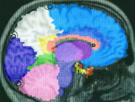
Example of the individualized template overlying an MRI scan. The approximate positions of the parasagittal and of the midsagittal landmarks (landmarks 1, 3, 4, and 6) are given with variability ellipses around them. The inner ellipse denotes the mean variability, in y and z direction, of the landmark position on the MRI versus the landmark position on the transformed template. The outer ellipse denotes the corresponding maximum variability.

Regional Values: Individual Subjects

In the TL orientation group, none of the regional values of [¹¹C] FMZ‐V_d lay outside the defined normal range. In the ACPC orientation group, a total of two values fell outside the normal range, one value for the left insula (+3.09 SD) and one for the right posterior cingulate gyrus (+3.14 SD). For the chosen thresholds and the 1292 values obtained (resulting from 38 regions × 34 subjects), less than four values would be predicted to fall outside the defined normal range; the data obtained is therefore in good agreement with the assumption of a normal distribution.

Comparison Between Image Orientations

The results (mean, SD, coefficient of variation) for each group are given in Table I. The average coefficient of variation (CV, defined as SD/Mean) across all regions was 0.13 in TL orientation and 0.16 in ACPC orientation. Average gray matter values of [¹¹C] FMZ‐V_d were not significantly different in ACPC or TL orientation. There were, however, significant differences between values derived in different orientations in 6/19 anatomical areas (Table I): parahippocampal gyrus (−13.5% in ACPC compared to TL orientation), fusiform gyrus (−18.3%), posterior cingulate gyrus (−12.5%), caudate nucleus (−18.9%), thalamus (−12.6%) and cerebellum (−15%).

DISCUSSION

We present the implementation, application and assessment of a versatile method for the quantification of brain imaging data. This method allows for the reliable definition of multiple cortical VOIs. The means and spread of the data obtained are comparable with traditional region‐of‐interest (ROI) analyses. At the same time, many of the pitfalls of ROI analyses are avoided: The process is entirely automated and therefore avoids intra‐ and inter‐rater subjectivity in the placement of regions. This has the added advantage of allowing repeated measurements over time without the drawbacks associated with user intervention. A further important advantage is speed. It is our experience that it takes a trained observer approximately 15 hr to manually outline all regions to sample an entire brain volume, whereas the spatial transformations undertaken in this study take less than 10 min. The method presented here can be used for the quantitation of MRI, magnetic resonance spectroscopy, PET, single photon emission tomography or other brain imaging data on a VOI basis, making it widely applicable.

Comparison With Previous Work

Approaches similar to ours have been described before [Bajcsy et al., 1983; Bohm et al., 1991; Christensen et al., 1997; Collins et al., 1999; Evans et al., 1988, 1991; Greitz et al., 1991; Kosugi et al., 1993]. The main difference to most of the earlier approaches are the complete automation of our protocol, with 100% reproducibility and no interobserver variability, and the use of a mature elastic matching protocol incorporating nonlinear transformations incorporated into SPM99 [Ashburner and Friston, 1999]. The spatial transformation module allows for the determination of the necessary warping steps from one image and their application to another one which is in register. As the T1 weighted MRI from which the anatomical template is derived is known, this can be exploited to transform the anatomical template with the same accuracy used in most current voxel‐based imaging studies. We have modified existing software from the SPM99 software package to reslice the spatially transformed template into any image space in register with the subject's MRI, e.g., a coregistered functional image, retaining the unequivocality of the assignment of voxels to regions through the use of nearest neighbor interpolation. To our knowledge, this computationally inexpensive and very efficient method has not been described previously.

A sophisticated method has been described recently, using a probabilistic atlas [Collins et al., 1999]. Individual data are transformed to the matrix of the atlas and the inverse transformation is used to transform the atlas back to the original image space for segmentation into VOIs. Although this ensures that the transformation is atlas‐independent, applying a dual transformation process is less efficient than using a single forward transformation from atlas space to individual space as in our approach. The atlas of Collins et al. [1999], has the advantage of using probabilistic information, but due to time constraints, the data used to build the atlas was itself automatically generated, with a similar protocol to that being tested. This may have introduced some bias. The only comparison made with manual subdivision was in the superior frontal gyrus. This is a relatively large structure, and no information on accuracy of mapping in other areas of the brain is obtained. It is to be expected, however, that the differences between the two approaches would be small in routine analyses in view of the similarity of the methods.

Construction of the Template

The algorithm for the manual subdivision of T1 weighted MRI scans was originally intended to be applied to all individual MRIs and therefore tested on five different datasets to provide unequivocal rules for delineation even in the presence of anatomical variants. As this version of the template is being used in studies of patients with epilepsy, we focussed our subdivisions on the temporal lobe [Koepp et al., 2000]. As the spatial transformation is independent of the actual atlas used, any other subdivision of the template can be used, and one may define further individual VOIs as needed for individual cases to address specific questions [Hu et al., 2000] or cluster some VOIs together [Hammers et al., 2001b].

The brain used to define our regional template has been used until recently (in SPM96) by the imaging community as a standard to which individual data has been normalized and therefore currently represents the best available substrate for the definition of standard regions. Ideally, however, such a regional template would not depend on individual anatomy but would incorporate some measure of variability between individuals, i.e., a probabilistic measure of region extent. This remains a desirable goal for the future [Mazziotta et al., 1995] but was not attempted here. One of the reasons is that it proved impossible to reliably outline smaller regions on the composite average brains as provided by the MNI and contained in the SPM99 package. We are currently in the process of manually segmenting a larger number of MRI scans, using the same algorithm, to obtain such an improved template.

Accuracy of Spatial Transformations

We show a 2D representation of a typical example with mean and maximum error ellipses in Figure 1. The spatial transformations were visually acceptable for all subjects in both orientations. Moreover, the formal evaluation indicated that the accuracy of the spatial transformations did not depend on the different angulation (about 35–40°) of the target images when the region template, created on an MRI in standard ACPC orientation, was transformed to the scans acquired in TL orientation. The parameters chosen for the transformations were thus sufficient to accommodate even relatively large deviations from the standard orientation of the original template. Our assessment of the spatial transformations used a landmark approach rather than measures of overlap. The accuracy data does not, therefore, indicate whether a particular landmark would always be assigned to the same VOI. This might be a problem in functionally distinct but anatomically close structures, as for example pre‐and postcentral gyrus. Figure 1 shows, however, that variability around the landmarks will only marginally affect the region sampled as a whole.

The accuracy of the superimposition of the anatomical regions onto the target brain volume was considered sufficient for cortical VOIs, considering the low resolution of most functional images (e.g., PET, single photon emission tomography or magnetic resonance spectroscopy). It has to be borne in mind that the accuracy data presented here depends not only on the ability of the spatial transformation process to match object template and target MRI but also on intersubject anatomical variability. In fact, the residual 3D distances between landmarks obtained with our protocol (approximately 7.5 mm on top of the intrarater variability for repeat measures) correspond well to the intersubject anatomical differences found by other workers for scans already registered into stereotaxic space with cross‐correlation methods [Collins et al., 1994] or with the AIR [Woods et al., 1993] algorithm [Grachev et al., 1999]. The latter method achieved somewhat smaller nominal values through the use of predefined planes for landmark placement, so that only two out of three coordinates could vary. Further refinement of shape matching algorithms such as SPM [Ashburner and Friston, 1999], AIR [Woods et al., 1993] and MNI_AutoReg/ANIMAL [Collins et al., 1994] may therefore not reduce this difference substantially, as it seems due to intersubject differences that are not reducible with these algorithms. It should be noted that this is the same inexactitude affecting voxel‐based studies.

We assessed the accuracy of the spatial transformations comparing landmarks determined on the subjects' MRI with those determined on the transformed template. As shown in Figure 1, the template tends to be slightly larger than the underlying brain. This is due to the way the template was constructed; we did not delineate the depth of intralobar sulci due to their expected positional differences in individual brains. This is likely to have slightly increased the Euclidean distances between landmarks given in Table II. When the VOI information from the spatially transformed template is combined with the anatomical information from the MRI to which it has been transformed, e.g., through multiplication of the individualised VOIs with the segmented MRI as in our example, the resulting accuracy will be further improved.

When quantification of brain imaging data in small and specific structures is sought, as for example in the hippocampus, millimetric precision may be required. It is prudent to outline these structures individually and add them onto the individualized template. This approach, however, requires the definition of criteria for the delineation of the anatomical structures in question and the subsequent validation of this protocol [Cook et al., 1992; Niemann et al., 2000]. A combination of speed and accuracy can be obtained by using our template approach for the fast delineation of a large number of regions with satisfactory precision and the individual delineation of small structures on MRI with optimum precision [Hammers et al., 2001b].

Characteristics of the Regional Data Obtained

The values of [¹¹C] FMZ binding obtained for cortical regions had descriptive characteristics similar to values obtained through traditional VOI analyses [Prevett et al., 1995]. The results obtained for basal ganglia in this study were generally poorer, as reflected by higher CVs. This may partly be due to segmentation into gray and white matter based on one T1 weighted MRI sequence alone; this is particularly relevant for the pallidum. Moreover, even minimal misplacement of the regions contained in the standard template will dramatically increase the variance, as these structures abut cerebrospinal fluid and white matter, with no or only nonspecific [¹¹C] FMZ binding. To obviate this problem, the basal ganglia could be individually delineated [Hu et al., 2000]. Another possibility would be to develop a PET‐to‐PET transformation with radioligands yielding a high signal in the basal ganglia, as for example the D₂‐receptor ligand [¹¹C] raclopride. Due to the better statistics with higher counts, this can significantly improve spatial normalization for the basal ganglia [Meyer et al., 1999].

Comparison of Regional Data Obtained From Functional Datasets in Different Orientations

Our results indicate that this method can be used for the analysis of brain imaging data acquired in different orientations: The regional values of [¹¹C] FMZ‐V_d were similar across orientations, although significant differences were observed in six out of 22 anatomical regions (parahippocampal gyrus, fusiform gyrus, posterior cingulate gyrus, caudate nucleus, thalamus and cerebellum). These are most likely due to the fact that our PET scanner produces anisotropic voxel sizes which may lead to different sampling of small and elongated regions like the majority of those for which we found differences [Mazziotta et al., 1981].

We aimed to directly compare regional values obtained and therefore used the absolute values for [¹¹C] FMZ‐V_d. It is apparent from the mean values that they tended to be higher in the temporal lobe orientation group, reflecting higher global signals. The difference in global signal explains the unidirectionality of the changes observed. As the regional values may be different for different orientations, control and patient data should be acquired in the same orientation.

In summary, we present a region template and a protocol for transforming that template to define anatomical volumes of interest (VOIs). The method described may be used to define anatomical VOIs in individual human brain imaging datasets without operator intervention. It is applicable to brain imaging data of different modalities or acquired in different orientations, and while generating regional data with characteristics similar to traditional region‐based analyses, it is completely observer‐independent and faster by a factor of about 90.

REFERENCES

- Ashburner J, Friston KJ (1997): Multimodal image coregistration and partitioning—a unified framework. NeuroImage 6: 209–217. [DOI] [PubMed] [Google Scholar]
- Ashburner J, Friston KJ (1999): Nonlinear spatial normalization using basis functions. Hum Brain Mapp 7: 254–266. [DOI] [PMC free article] [PubMed] [Google Scholar]
- Bailey DL (1992): Three dimensional acquisition and reconstruction in positron emission tomography. Ann Nucl Med 6: 121–130. [DOI] [PubMed] [Google Scholar]
- Bailey DL, Meikle SR (1994): A convolution‐subtraction scatter correction method for 3D PET. Phys Med Biol 39: 411–424. [DOI] [PubMed] [Google Scholar]
- Bajcsy R, Lieberson R, Reivich M (1983): A computerized system for the elastic matching of deformed radiographic images to idealised atlas images. J Comput Assist Tomogr 7: 618–625. [DOI] [PubMed] [Google Scholar]
- Bohm C, Greitz T, Seitz R, Eriksson L (1991): Specification and selection of regions of interest (ROIs) in a computerized brain atlas. J Cereb Blood Flow Metab 11: A64–A68. [DOI] [PubMed] [Google Scholar]
- Christensen GE, Joshi SC, Miller MI (1997): Volumetric transformation of brain anatomy. IEEE Trans Med Imaging 16: 864–877. [DOI] [PubMed] [Google Scholar]
- Collins DL, Neelin P, Peters TM, Evans AC (1994): Automatic 3D intersubject registration of MR volumetric data in standardized Talairach space. J Comput Assist Tomogr 18: 192–205. [PubMed] [Google Scholar]
- Collins DL, Zijdenbos AP, Baaré WFC, Evans AC. 1999. ANIMAL+INSECT: Improved cortical structure segmentation. LNCS 1613: 210–223. [Google Scholar]
- Collins DL, Zijdenbos AP, Kollokian V, Sled JG, Kabani NJ, Holmes CJ, Evans AC (1998): Design and construction of a realistic digital brain phantom. IEEE Trans Med Imaging 17: 463–468. [DOI] [PubMed] [Google Scholar]
- Cook MJ, Fish DR, Shorvon SD, Straughan K, Stevens JM (1992): Hippocampal volumetric and morphometric studies in frontal and temporal lobe epilepsy. Brain 115: 1001–1015. [DOI] [PubMed] [Google Scholar]
- Cunningham VJ, Jones T (1993): Spectral analysis of dynamic PET data. J Cereb Blood Flow Metab 13: 15–23. [DOI] [PubMed] [Google Scholar]
- Evans AC, Beil C, Marrett S, Thompson CJ, Hakim A (1988): Anatomical‐functional correlation using an adjustable MRI‐based region of interest atlas with positron emission tomography. J Cereb Blood Flow Metab 8: 513–530. [DOI] [PubMed] [Google Scholar]
- Evans AC, Marett S, Torrescorzo J, Ku S, Collins L (1991): MRI‐PET correlation in three dimensions using a volume‐of‐interest (VOI) atlas. J Cereb Blood Flow Metab 11: A69–A78. [DOI] [PubMed] [Google Scholar]
- Friston KJ, Ashburner J, Poline JB, Frackowiak RSJ (1995): Spatial registration and normalisation of images. Hum Brain Mapp 2: 165–189. [Google Scholar]
- Grachev ID, Berdichevsky D, Rauch SL, Heckers S, Kennedy DN, Caviness VS, Alpert NM (1999): A method for assessing the accuracy of intersubject registration of the human brain using anatomic landmarks. NeuroImage 9: 250–268. [DOI] [PubMed] [Google Scholar]
- Greitz T, Bohm C, Holte S, Eriksson L (1991): A computerized brain atlas: construction, anatomical content, and some applications. J Comput Assist Tomogr 15: 26–38. [PubMed] [Google Scholar]
- Grootoonk S (1995): Dual energy window correction for scattered photons in 3D positron emission tomography. PhD Thesis. University of Surrey, Guildford, Surrey.
- Hammers A, Koepp MJ, Labbé C, Brooks DJ, Thom M, Cunningham VJ, Duncan JS (2001a): Neocortical abnormalites of [11C]‐flumazenil PET in mesial temporal lobe epilepsy. Neurology 56: 897–906. [DOI] [PubMed] [Google Scholar]
- Hammers A, Koepp MJ, Richardson MP, Labbé C, Brooks DJ, Cunningham VJ, Duncan JS (2001b): Central benzodiazepine receptors in malformations of cortical development. A quantitative study. Brain 124: 1555–1565. [DOI] [PubMed] [Google Scholar]
- Hartigan JA (1975): Clustering algorithms. New York: John Wiley & Sons, Inc. 351 p. [Google Scholar]
- Holmes CJ, Hoge R, Collins L, Woods R, Toga AW, Evans AC (1998): Enhancement of MR images using registration for signal averaging. J Comput Assist Tomogr 18: 192–205. [DOI] [PubMed] [Google Scholar]
- Hu MT, Taylor‐Robinson SD, Chaudhuri KR, Bell JD, Labbé C, Cunningham VJ, Koepp MJ, Hammers A, Morris RG, Turjanski N, Brooks DJ (2000): Cortical dysfunction in non‐demented Parkinson's disease patients. A combined 31P‐MRS and 18FDG‐PET study. Brain 123: 340–352. [DOI] [PubMed] [Google Scholar]
- Jackson GD, Berkovic SF, Duncan JS, Connelly A (1993): Optimizing the diagnosis of hippocampal sclerosis using MR imaging. Am J Neuroradiol 14: 753–762. [PMC free article] [PubMed] [Google Scholar]
- Kiebel SJ, Ashburner J, Poline JB, Friston KJ (1997): ); MRI and PET coregistration—a cross validation of statistical parametric mapping and automated image registration. NeuroImage 5: 271–279. [DOI] [PubMed] [Google Scholar]
- Koepp MJ, Hammers A, Labbé C, Wörmann FG, Brooks DJ, Duncan JS (2000): 11C‐flumazenil PET in patients with refractory temporal lobe epilepsy and normal MRI. Neurology 54: 332–339. [DOI] [PubMed] [Google Scholar]
- Koepp MJ, Richardson MP, Brooks DJ, Poline JB, Van Paesschen W, Friston KJ, Duncan JS (1996): Cerebral benzodiazepine receptors in hippocampal sclerosis. An objective in vivo analysis. Brain 119: 1677–1687. [DOI] [PubMed] [Google Scholar]
- Koeppe RA, Holthoff VA, Frey KA, Kilbourn MR, Kuhl DE (1991): Compartmental analysis of [11C] flumazenil kinetics for the estimation of ligand transport rate and receptor distribution using positron emission tomography. J Cereb Blood Flow Metab 11: 735–744. [DOI] [PubMed] [Google Scholar]
- Kosugi Y, Sase M, Kuwatani H, Kinoshita N, Momose T, Nishikawa J, Watanabe T (1993): Neural network mapping for nonlinear stereotactic normalization of brain MR images. J Comput Assist Tomogr 17: 455–460. [DOI] [PubMed] [Google Scholar]
- Labbé C, Koepp MJ, Ashburner J, Spinks TJ, Richardson MP, Duncan JS, Cunningham VJ (1998): Absolute PET quantification with correction for partial volume effects within cerebral structures In: Carson C, Daube‐Witherspoon M, Herscovitch P, editors. Quantitative functional brain imaging with positron emission tomography. San Diego: Academic Press; p 59–66. [Google Scholar]
- Maes F, Collignon A, Vandermeulen D, Marchal G, Suetens P (1997): Multimodality image registration by maximazation of mutual information. IEEE Trans Med Imaging 16: 187–198. [DOI] [PubMed] [Google Scholar]
- Mazziotta JC, Phelps ME, Plummer D, Kuhl DE (1981): Quantitation in positron emission tomography: 5. Physical‐anatomical effects. J Comput Assist Tomogr 3: 299–308. [DOI] [PubMed] [Google Scholar]
- Mazziotta JC, Toga AW, Evans AC, Fox P, Lancaster J (1995): A probabilistic atlas of the human brain: theory and rationale for its development. NeuroImage 2: 89–101. [DOI] [PubMed] [Google Scholar]
- Meyer JH, Gunn RN, Myers R, Grasby PM (1999): Assessment of spatial normalization of PET ligand images using ligand‐specific templates. NeuroImage 9: 545–553. [DOI] [PubMed] [Google Scholar]
- Müller Gartner HW, Links JM, Prince JL, Bryan RN, McVeigh E, Leal JP, Davatzikos C, Frost JJ (1992): Measurement of radiotracer concentration in brain gray matter using positron emission tomography: MRI‐based correction for partial volume effects. J Cereb Blood Flow Metab 12: 571–583. [DOI] [PubMed] [Google Scholar]
- Niemann K, Hammers A, Coenen VA, Thron A, Klosterkötter J (2000): Evidence for smaller left hippocampus and left temporal horn in both patients with first episode schizophrenia and normal controls. Psychiatry Res Neuroimaging 99: 93–110. [DOI] [PubMed] [Google Scholar]
- Press GA, Amaral DG, Squire LR (1989): Hippocampal abnormalities in amnesic patients revealed by high‐resolution magnetic resonance imaging. Nature 341: 54–57. [DOI] [PubMed] [Google Scholar]
- Prevett MC, Lammertsma AA, Brooks DJ, Bartenstein PA, Patsalos PN, Fish DR, Duncan JS (1995): Benzodiazepine‐GABAA receptors in idiopathic generalised epilepsy measured with [11C]flumazenil and positron emission tomography. Epilepsia 36: 113–121. [DOI] [PubMed] [Google Scholar]
- Richardson MP, Friston KJ, Sisodiya SM, Koepp MJ, Ashburner J, Free SL, Brooks DJ, Duncan JS (1997): Cortical grey matter and benzodiazepine receptors in malformations of cortical development. A voxel‐based comparison of structural and functional imaging data. Brain 120: 1961–1973. [DOI] [PubMed] [Google Scholar]
- Rousset OG, Ma Y, Léger GC, Gjedde AH, Evans AC (1993): Correction for partial volume effects in PET using MRI‐based 3D simulations of individual human brain metabolism In: Uemura K, editor. Quantification of brain function, tracer kinetics and image analysis in brain PET. New York, NY: Elsevier Science; p 113–125. [Google Scholar]
- Ryvlin P, Bouvard S, Le Bars D, De Lamérie G, Grégoire MC, Kahane P, Froment JC, Mauguière F. 1998. Clinical utility of flumazenil‐PET vs. [18F] fluorodeoxyglucose‐PET and MRI in refractory partial epilepsy. A prospective study in 100 patients. Brain 121: 2067–2081. [DOI] [PubMed] [Google Scholar]
- Strul D, Bendriem B (1999): Robustness of anatomically guided pixel‐by‐pixel algorithms for partial volume effect correction in positron emission tomography. J Cereb Blood Flow Metab 19: 547–559. [DOI] [PubMed] [Google Scholar]
- Studholme C, Hill DLG, Hawkes DJ (1997): Automated 3D registration of magnetic resonance and positron emission tomography brain images by multiresolution optimization of voxel similarity measures. Med Phys 24: 25–35. [DOI] [PubMed] [Google Scholar]
- van den Elsen PA, Pol E‐JD, Viergever MA (1993): Medical image matching—a review with classification. IEEE Eng Med Biol 12: 26–39. [Google Scholar]
- Van Paesschen W, Connelly A, King MD, Jackson GD, Duncan JS (1997): The spectrum of hippocampal sclerosis: a quantitative magnetic resonance imaging study. Ann Neurol 41: 41–51. [DOI] [PubMed] [Google Scholar]
- Woods RP, Mazziotta JC, Cherry SR (1993): MRI‐PET registration with automated algorithm. J Comp Assist Tomogr 17: 536–546. [DOI] [PubMed] [Google Scholar]