Determination of individual stimulus–response curves in the visual cortex

Abstract

Activation in the visual cortex is typically studied using group average changes in an on–off paradigm for a single flicker frequency. We used functional magnetic resonance imaging (fMRI) to characterize the stimulus–response curve in the visual cortex as a function of flicker frequency in individual subjects, using LED goggles with 17 frequency steps between 0 and 30 Hz. Ten healthy young individuals were studied on two different occasions (mean interval; 22 days). In all but one subject, a third‐order polynomial curve could be fitted to the data. From the response curve we calculated the peak response (the frequency where the response amplitude was maximal), the percentage change (relative difference) of the response amplitudes between 8 Hz and the peak frequency, and the average slope of response (towards the peak). On both occasions we could determine a peak response for each subject with small within‐subject variability. The average absolute difference in peak response between both sessions was 1.37 Hz (range, 0.2–4.3 Hz), indicating that the peak frequency is rather stable for a given individual. In conclusion, our study illustrates the ability of fMRI to examine the stimulus–response curve in individual subjects in the visual cortex. Based on our findings, the peak response and the slope of response seem highly reproducible within subjects. A similar analysis of the stimulus–response curve may be applicable to other types of stimuli. Hum. Brain Mapping 17:245–251, 2002. © 2002 Wiley‐Liss, Inc.

INTRODUCTION

In recent years, numerous functional magnetic resonance imaging (fMRI) and positron emission tomography (PET) studies have used flashing light as a stimulus to examine neuronal activity in the visual cortex. Activation in the visual cortex is typically studied using group average changes in an on–off paradigm for a single flicker frequency. Studies that applied parametric designs, where in the frequency of the lightflashes was varied, showed that the response increases with increasing frequency, with maximum responses reported around 8 Hz [Fox and Raichle, 1984; Kwong et al., 1992; Mentis et al., 1997, 1998; Thomas and Menon, 1998; Zhu et al., 1998]. At higher frequencies, the response decreases again. In these studies, the average signal of a group of subjects was reported, whereas the response as a function of flicker frequency might differ between subjects.

fMRI offers the possibility to study in each individual the response curve as a function of flicker frequency and also the reproducibility of this response. We apply fMRI to study whether reproducible blood oxygenation level dependent (BOLD) response curves can be determined as a function of flicker frequency in individual subjects. We hypothesize that the frequency of maximal amplitude of response differs between individuals.

METHODS

Subjects

Ten healthy students and graduates (6 male, 4 female), free from neurological disorders and visual abnormalities, participated in this study. Mean age was 22.9 years (range, 21–26 years). The subjects were studied on two separate occasions, using a full parametrical design with an interval of 5 days to 7 weeks (mean, 22 days). Directly after the second session, a third session was carried out to determine the area of the visual cortex using an on–off paradigm.

Data acquisition

A 1.5 T MR scanner (Vision; Siemens, Erlangen, Germany) was used, equipped with a standard circularly polarized head coil. To restrict head movement foam padding was used. Before functional scanning, a scout image was obtained. For fMRI, a gradient echo, echo planar imaging (EPI) sequence was used (repetition time [TR]: 2.275 sec, echo time [TE]: 60 msec, flip angle: 90 degrees, matrix size: 64 × 64, field of view [FOV]: 192 × 192 mm², slice thickness: 5 mm, interslice gap: 1 mm). EPI scans were acquired in an axial plane to cover the whole brain. Structural imaging included a T1‐weighted 3D gradient echo sequence (MPRAGE: inversion time: 300 msec, TR: 15 msec, TE: 7 msec, flip angle: 8 degrees, matrix: 256 × 256, FOV: 250 × 250 mm³, slice thickness: 1.5 mm, number of slices typically 120), oriented coronally.

Task

For visual stimulation, standard goggles were used (S10VSB; Grass Instruments, Quincy, MA), with a 5 × 6 red LED matrix in front of each eye. The photic stimuli, mean peak 640 nm, subtended degrees approximately 45 degrees of arc. The goggles were adjusted for personal comfort; no outside light could enter. The subjects were instructed to lie still and to keep their eyes open for the duration of the task. The visual eye fields were stimulated bilaterally with a flicker frequency that increased parametrically (first and second session). The flicker frequency was varied by changing the duration between flashes, with a fixed duration of the flashes (5 msec). Therefore, the luminous intensity per time unit increased as flicker frequency increased. Twenty scans were made in total darkness, followed by 17 blocks of 15 scans each, with flicker frequencies of 0.25, 0.50, 1, 2, 4, 6, 8, 10, 12, 14, 16, 18, 20, 22, 24, 26, and 30 Hz. The same parametrical design was administered in both the first and second scanning session. The presentation of these flicker frequencies was not randomized or counterbalanced across subjects; the time required for a photoreceptor to recover its dark‐level response characteristics is within 5–10 min [Roof and Heth, 1994]. For example, when the 2‐Hz flicker frequency would follow the 24‐Hz flicker frequency, several minutes of rest would be required to attain physiological habituation, rendering randomization of 18 different flicker frequencies unrealistic. During the third session, we applied an on–off flicker presentation task (8 Hz and 0 Hz). In the first block, 15 scans were made during an 8‐Hz flicker frequency, followed by seven blocks of 10 scans each, alternating in flicker frequency between 0 and 8 Hz. These data were acquired to locate in each individual the region of interest (ROI) in the visual cortex for the parametrical data analysis.

Data analysis

For data analysis, SPM99 [Friston et al., 1995] and AFNI [Cox, 1996] were used. The first five scans of each task were discarded, no transition scans between frequencies were discarded. All volumes were corrected for motion and repositioning, by realigning them to the first scan of the first study, in native space. The structural scan was coregistered to the EPI volumes. The EPI scans and the structural scans were resliced to 3‐mm and 1‐mm isotropic voxels, respectively.

In all calculations, a two‐scan delay was used to account for the delay in the hemodynamic response. First, to locate the functional area within the visual cortex, the activation map from the on–off paradigm (third session) was computed by correlating each voxel's time course with a boxcar alternating with the same on–off frequency. Our approach was to determine response curves in individual ROIs of the visual cortex, defined by voxels that showed a highly significant effect during the on–off paradigm (Fig. 1). Therefore, the correlation threshold was set at a stringent P‐value (P = 10⁻¹⁰), corresponding to a correlation value of 0.64 [Cox, 1996]. For an accurate inspection of the localization of the activated area within the visual cortex, the structural scans were used. In each subject, the ROI was then manually drawn upon the EPI images in the center of the activated area; care was taken not to include large venous structures (e.g., straight sinus). The size and localization of activity within the visual cortex was unique for each subject, as were the ROIs. Rombouts et al. [1998] found a good reproducibility of the size and overlap of activated volume when using an 8‐Hz flicker stimulus to activate the visual cortex. Therefore, for each subject, the same ROIs were applied to the first and second session. These ROIs, derived in the third session, defined the functionally most active area in the visual cortex and were used to analyze the stimulus–response curves as a function of flicker frequency (first and second session). For each parametrical data set, the time course of all voxels contained in the ROIs was first averaged and the mean was scaled to 100. The average signal intensity per frequency (mean, 15 time points/frequency) was computed. A third‐order polynomial fit was applied to these average signal intensities to determine the response curve. A correlation coefficient was computed between the points of the two response curves for both scanning sessions. From the third‐order polynomial fit we determined three parameters: 1) the frequency of peak response; 2) the difference in signal intensity between peak and 8 Hz; and 3) the average upward slope. The absolute difference between the frequencies of peak response for both sessions was computed for each subject. The reproducibility of the three parameters was computed for both sessions for each individual. For all scan–rescan analyses a reproducibility ratio (R¹²) was computed [Rombouts et al., 1998], which varies between 0.0 (worst) and 1.0 (best). This ratio characterizes how well measures of activation are reproduced between sessions.

Figure 1.

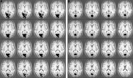
Raw activation map showing the visual cortex using the 8‐Hz on–off paradigm on 16 successive slices (A) and the corresponding manually drawn ROIs that were used for the parametric analysis (B).

An overall stimulus–response curve using group‐averaged data was computed for both the first and second session. Again a third‐order polynomial fit was applied to these average signal intensities. From this fit the peak of response was determined for comparison purposes with other studies using group‐averaged data.

RESULTS

In all 10 subjects, activation was detected in expected areas in the visual cortex with the on–off paradigm, using a correlation value of 0.64 (P = 10⁻¹⁰). The size of activation in the visual cortex, however, is different for each subject [Rombouts, 1998]. Using a simple light‐flash stimulus in the present study, we can see where the activation should be localized (in contrast to more complex stimuli). The selected threshold can therefore be changed for each subject to obtain the functionally most active area in the visual cortex of comparable size and localization. In one subject, the correlation value had to be decreased to 0.50 (P = 2.7 × 10⁻⁶) to detect a functional area of comparable size and localization to the other nine subjects. The average size of the manually drawn ROIs was 4.5 cm³ (range 3.2 cm³–7.3 cm³). In nine subjects (in both sessions), an increase in signal intensity, peak and then a decrease in signal intensity could be observed (Fig. 2), as shown by others in group averaged data [Fox and Raichle, 1984; Kwong et al., 1992; Mentis et al., 1997, 1998; Thomas and Menon, 1998; Zhu et al., 1998]. In one subject, no acceptable fit of the data could be obtained even though the functional area of the visual cortex yielded a normal response in the on–off paradigm (at P = 10⁻¹⁰). In the remaining nine subjects, an average goodness‐of‐fit (R²) of 0.90 (range, 0.80–0.96) was found for the first session and an R² of 0.86 (range, 0.75–0.98) for the second session (Table I).

Figure 2.

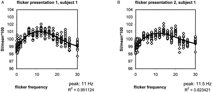
Signal intensity (SI) changes in one subject for the first (A) and second (B) parametrical flicker presentation task. Open white squares represent a single time‐scan point. Filled black squares represent the average SI for each frequency. A polynomial curve could be fitted to the average timepoints of each frequency, showing the characteristics of the blood response.

Table I.

Peak responses, percentages change 8 Hz versus peak response, slopes of response and the goodness of fit of 9 subjects

Subject no.	Flicker task	Peak (Hz)	Δ SI peak (%)	Δ SI at 8 Hz (%)	Δ Peak vs. 8 Hz (%)	Average upward slope (%/Hz)	R2‐value (goodness of fit)
1	First	11.0	2.228	2.093	0.135	0.203	0.951
	Second	11.5	1.822	1.683	0.139	0.158	0.823
2	First	12.8	2.487	2.200	0.287	0.194	0.798
	Second	13.0	1.632	1.433	0.199	0.126	0.753
3	First	12.5	2.855	2.570	0.285	0.228	0.831
	Second	14.1	4.272	3.603	0.669	0.303	0.929
4	First	11.3	2.002	1.860	0.142	0.177	0.926
	Second	10.0	1.174	1.136	0.038	0.117	0.803
5	First	11.3	1.659	1.546	0.113	0.147	0.939
	Second	10.8	1.549	1.464	0.085	0.143	0.955
6	First	11.0	2.407	2.274	0.133	0.219	0.904
	Second	12.5	1.599	1.433	0.166	0.128	0.839
7	First	10.7	1.763	1.677	0.086	0.165	0.939
	Second	15.0	2.361	1.914	0.447	0.157	0.983
8	First	12.5	2.613	2.349	0.264	0.209	0.887
	Second	11.9	1.574	1.435	0.139	0.132	0.897
9	First	11.1	2.532	2.376	0.156	0.228	0.964
	Second	9.3	1.953	1.922	0.031	0.210	0.793
Average first		11.58 ± 0.79	2.28 ± 0.40	2.10 ± 0.34	0.18 ± 0.08	0.20 ± 0.03	0.90 ± 0.06
Median first		11.3	2.41	2.2	0.142	0.203	0.926
Average second		12.01 ± 1.86	1.99 ± 0.91	1.78 ± 0.73	0.21 ± 0.21	0.16 ± 0.06	0.86 ± 0.08
Median second		13	1.63	1.464	0.139	0.143	0.839

The frequency of peak response varied between 9.3 and 15.0 Hz. In the first session we found an average peak response at 11.6 Hz (range, 10.7–12.8 Hz). The percentage signal change between 8 Hz and the frequency of peak response showed an average increase of 0.18% (range, 0.09–0.29). The average upward slope for the first session was 0.20%/Hz (range, 0.15–0.23). For the second session, an average peak response was found at 12.0 Hz (range, 9.3–15 Hz), the percentage change between 8 Hz and peak was 0.21% (range, 0.03–0.67). The average slope was 0.16%/Hz (range, 0.12–0.30%/Hz) (Table I).

The average correlation coefficient between the two response curves (first and second session) in each individual was 0.85 (range, 0.73–0.92 for individual frequencies). The reproducibility measures for the nine subjects showed an average absolute difference in frequency of peak response between the first and second study of 1.37 Hz (range, 0.2–4.3 Hz). R¹² for the peak frequency showed an average value of 0.94 (range, 0.83–0.99). The average increase in signal intensity between 8 Hz and the peak response in both studies was 0.14% (range, 0.00–0.38%) with an average R¹² of 0.66 (range, 0.32–0.99). The average difference in slope of response between the two studies was 0.05%/Hz (range, 0.00–0.09%/Hz), with an average reproducibility ratio of 0.86 (range, 0.74–0.99). The reproducibility of the amplitude of the frequency of peak response was 0.83 (range, 0.74–0.97) and at 8 Hz 0.84 (range 0.76–0.97). Finally, the overall (n = 9) stimulus–response curve averaged over all subjects revealed for the first session (R² of 0.96) a peak response at 11.6 Hz and for the second session (R² of 0.96) a peak response at 12.0 Hz (Fig. 3).

Figure 3.

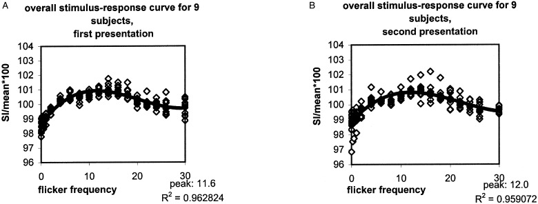
Average stimulus–response curve across nine subjects for the first (A) and the second (B) parametrical flicker presentation task. Open white squares represent average SI for each subject at each frequency. Filled black squares represent the overall average SI for each frequency for nine subjects. The polynomial curve could be fitted to the overall average SI for each frequency, showing the peak response.

DISCUSSION

In this fMRI study, we used LED goggles to apply a parametrical flicker task in 10 healthy students to estimate a stimulus–response curve as a function of increasing flicker frequency in the visual cortex. For nine of 10 subjects, acceptable curves could be fitted to the data of individual subjects allowing accurate and reproducible stimulus–response curves to be determined.

In contrast to earlier studies, particularly those carried out using PET, we were able to derive stimulus–response curves in individual subjects. The average peak response found here was higher than in other studies, each of which showed an average peak around 8 Hz [Fox and Raichle, 1984; Kwong et al., 1992; Mentis et al., 1997, 1998; Thomas and Menon, 1998; Zhu et al., 1998]. There are six major factors that might cause this difference: 1) The presentation of the flicker frequencies used in the present study were not randomized or counterbalanced across subjects. The adaptation effect resulting from this design is likely to explain the differences found in peak response compared to other studies. When, for example, a low flicker frequency would follow a high flicker frequency, several minutes of rest would be required for physiological habituation [Roof and Heth, 1994]. Randomization of 18 different flicker frequencies would therefore be unrealistic. Because no periods of rest were inserted in our design, habituation effects were likely to play a role. 2) Because all frequencies were presented in an increasing order, an additional attention effect could have biased the tuning curve. 3) We determined the frequency of the light flashes by varying the time between flashes. Because the flash duration was fixed at 5 msec, the duty cycle changed for each frequency. This may have biased the results by introducing higher frequency harmonics in the data. 4) The primary and secondary visual fields were not distinguished in the selected ROIs. It is still unclear whether different visual areas have different temporal tuning characteristics [Chawla et al., 1998; Singh et al., 2000]. Different temporal tuning characteristics between visual areas could attribute to differences found in stimulus–response curves. Noll et al. [1997] present a statistical technique to evaluate the classification process for determining which voxels are active or inactive. They state that multiple (four repetitions or more are advisory) runs give better estimates. Because we administered a flicker task on two occasions, we used an additional activation map to determine the active region within the visual cortex. 5) A different stimulation method could also explain the difference in peak response. For example, the number of LEDs, the distance from LEDs to the eyes and the luminance are not the same in all studies. 6) The large steps between successive frequencies and the small amount of frequencies used in earlier studies might have resulted in undersampling of the response curve; we used a large number of small steps between frequencies, enabling us to accurately determine the stimulus–response curve. Note, however, that the goal of the study was not to reveal the “true” peak response but to determine a detailed individual stimulus–response curve and to examine the reproducibility of these curves within subjects.

The visual system has been investigated in many studies to understand and reveal some of the physiological mechanisms underlying the response characteristics. The peak response reflects the highest neuronal activity [Fox and Raichle, 1985], which in turn reflects the activity–recovery cycle of cells in the retina [Bartley, 1968]. Ozus et al. [2001] show time courses of BOLD signal changes in the primary visual cortex at different flicker frequencies, averaged across subjects. Their data show an increase in BOLD signal with stimulation frequency from 0–6 Hz. At frequencies higher than 6 Hz, the signal shows a plateau, suggesting a saturation effect. Glucose utilization reaches a peak at flicker frequencies of 15 Hz and higher during electrical stimulation [Yarowsky, 1983], therefore placing an upper limit to the peak response. In addition, there might be a correlation between large‐amplitude evoked potentials and a subject's alpha‐rhythm, which varies between 8 and 13 Hz [Niedermeyer, 1982]. The peak responses found in the current study are within this range and vary between subjects as expected.

One objective of our study was to determine the reproducibility of the peak response and the other characteristics of the time course in each individual. To determine the reproducibility, each subject was tested twice, with an average of 22 days time interval. The average absolute difference in peak frequency between the first and second flicker task was 1.37 Hz (range, 0.2–4.3 Hz), with a high average reproducibility (R¹² = 0.94; range, 0.83–0.99). The difference in signal intensity from 8 Hz to the frequency of the peak response showed more variation between the first and second flicker task: average difference of 0.14% (range, 0.00–0.38) between sessions, and an R¹² of 0.66 (range, 0.32–0.99). The average difference for the slope of response between the two flicker sessions was 0.05%/Hz (range, 0.00–0.09), with a good reproducibility ratio of 0.86 (range, 0.74–0.99) (Table I). These results show that the peak response and the slope of response are reproducible within subjects. Although we did not set up our study to compare response variability within subjects to variability between subjects, our data suggest that these variabilities are comparable (Table I). For a proper variability comparison, each subject should ideally undergo as many repeated scans as the number of subjects present in the study (in our case 10).

In conclusion, our study illustrates the ability of fMRI to determine the stimulus–response curve in individual subjects in the functional visual cortex. These findings underline the unique sensitivity of BOLD fMRI allowing extensive parameterization. We speculate that such extensive parametrizations will be useful when studying more complex (cognitive) stimuli, because they might reveal more variance in the location of the peak response than for simple (sensory) stimuli, such as light flashes. When substantiated, stimulus–response curve analysis could be used to understand, and control for, the marked interindividual variations typically observed for cognitive tasks using a single stimulus intensity in an on–off design.

REFERENCES

- Bartley SH (1968): Temporal features of input as crucial factors in vision In: Neff WD, ed. Contributions to sensory physiology. New York: Academic Press; p 81–124. [PubMed] [Google Scholar]
- Chawla D, Phillips J, Buechel C, Edwards R, Friston KJ (1998): Speed‐dependent motion‐sensitive responses in V5: an fMRI study. Neuroimage 7: 86–96. [DOI] [PubMed] [Google Scholar]
- Cox RW (1996): AFNI: software for analysis and visualization of functional magnetic resonance neuroimages. Comput Biomed Res 29: 162–173. [DOI] [PubMed] [Google Scholar]
- Fox PT, Raichle ME (1984): Stimulus rate dependence of regional cerebral blood flow in human striate cortex, demonstrated by positron emission tomography. J Neurophysiol 51: 1109–1120. [DOI] [PubMed] [Google Scholar]
- Friston KJ, Holmes AP, Worsley KJ, Poline JB, Frith CD (1995): Statistical parametric maps in functional imaging: a general linear approach. Hum Brain Mapp 2: 189–210. [Google Scholar]
- Kwong KK, Belliveau JW, Chesler DA, Goldberg IE, Weisskoff RM, Poncelet BP, Kennedy DN, Hoppel BE, Cohen MS, Turner R, Cheng HM, Brady TJ, Rosen BR (1992): Dynamic magnetic resonance imaging of human brain activity during primary sensory stimulation. Proc Natl Acad Sci U S A 89: 5675–5679. [DOI] [PMC free article] [PubMed] [Google Scholar]
- Mentis MJ, Alexander GE, Grady CL, Horwitz B, Krasuski J, Pietrini P, Strassburger T, Hampel H, Schapiro MB, Rapoport SI. (1997): Frequency variation of a pattern‐flash visual stimulus during PET differentially activates brain from striate through frontal cortex. Neuroimage 5: 116–128. [DOI] [PubMed] [Google Scholar]
- Mentis MJ, Alexander GE, Krasuski J, Pietrini P, Furey ML, Schapiro MB, Rapoport SI (1998): Increasing required neural response to expose abnormal brain function in mild versus moderate or severe Alzheimer's disease: PET study using parametric visual stimulation. Am J Psychiatry 155: 785–794. [DOI] [PubMed] [Google Scholar]
- Niedermeyer E (1982): The normal EEG of the waking adult In: Niedermeyer E, Lopes da Silva F, eds. Electroencephalography. Baltimore: Urban and Schwarzenberg; p 71–91. [Google Scholar]
- Noll DC, Genovese CR, Nystrom LE, Vasquez AL, Forman SD, Eddy WF, Cohen JD (1997): Estimating test‐retest reliability in functional MR imaging II: application to motor and cognitive activation studies. Magn Reson Imaging 38: 508–517. [DOI] [PubMed] [Google Scholar]
- Ozus B, Liu HL, Chen L, Iyer MB, Fox PT, Gao JH (2001): Rate dependence of human visual cortical response due to brief stimulation: an event‐ralated fMRI study. Magn Reson Imaging 19: 21–25. [DOI] [PubMed] [Google Scholar]
- Regan D (1972): Evoked potentials in psychology, sensory physiology and clinical medicine. London: Chapman and Hall. [Google Scholar]
- Rombouts SARB, Barkhof F, Hoogenraad FGC, Sprenger M, Scheltens P (1998): Within‐subject reproducibility of visual activation patterns with functional magnetic resonance imaging using multislice echo planar imaging. Magn Reson Imaging 16: 105–113. [DOI] [PubMed] [Google Scholar]
- Roof DJ, Heth CA (1994): Photoreceptors and retinal pigment epithelium transduction and renewal mechanisms In: Albert DM, Jakobiec FA, eds. Principles and practice of ophthalmology. Philadelphia: Saunders Company; p 309–331. [Google Scholar]
- Singh KD, Smith AT, Greenlee MW (2000): Spatio‐temporal frequency and direction sensitivities of human visual areas measured using fMRI. Neuroimage 12: 550–564. [DOI] [PubMed] [Google Scholar]
- Thomas CG, Menon RS (1998): Amplitude response and stimulus presentation frequency response of human primary visual cortex using BOLD EPI at 4 T. Magn Reson Med 40: 203–209. [DOI] [PubMed] [Google Scholar]
- Yarowsky P, Kadekaro M, Sokoloff L (1983): Frequency‐dependent activation of glucose utilization in the superior cervical ganglion by electrical stimulation of cervical sympathetic trunc. Proc Acad Natl Sci U S A 80: 4179–4183. [DOI] [PMC free article] [PubMed] [Google Scholar]
- Zhu XH, Kim SG, Andersen P, Ogawa S, Ugurbil K, Chen W (1998): Simultaneous oxygenation and perfusion imaging study of functional activity in primary visual cortex at different visual stimulation frequency: quantitative correlation between BOLD and CBF changes. Magn Reson Med 40: 703–711. [DOI] [PubMed] [Google Scholar]