

Abstract
The study of dynamic interdependences between brain regions is currently a very active research field. For any connectivity study, it is important to determine whether correlations between two selected brain regions are statistically significant or only chance effects due to non‐specific correlations present throughout the data. In this report, we present a wavelet‐based non‐parametric technique for testing the null hypothesis that the correlations are typical of the data set and not unique to the regions of interest. This is achieved through spatiotemporal resampling of the data in the wavelet domain. Two functional MRI data sets were analysed: (1) Data from 8 healthy human subjects viewing a checkerboard image, and (2) “Null” data obtained from 3 healthy human subjects, resting with eyes closed. It was demonstrated that constrained resampling of the data in the wavelet domain allows construction of bootstrapped data with four essential properties: (1) Spatial and temporal correlations within and between slices are preserved, (2) The irregular geometry of the intracranial images is maintained, (3) There is adequate type I error control, and (4) Expected experiment‐induced correlations are identified. The limitations and possible extensions of the proposed technique are discussed. Hum. Brain Mapp. 23:1–25, 2004. © 2004 Wiley‐Liss, Inc.
Keywords: functional connectivity, wavelet transform, surrogate data, brain dynamics, bootstrapping, resampling
INTRODUCTION
The nature and significance of dynamic interactions between brain regions is currently an important focus of neuroscience research [for review see Varela et al., 2001]. Such interactions are postulated to coordinate, integrate, and constrain the expression of neural activity across multiple functional networks [e.g., Peled 1999] and hence may be crucial to brain function. This research requires techniques for the accurate identification and description of spatial and temporal correlations in brain imaging data [Friston et al., 1993, Schiff et al., 1996]. Two steps are required: (1) A method of quantifying correlations that is best suited to the type of interactions (e.g., linear or nonlinear) of interest, and (2) A technique of estimating the expected distribution of such correlations under the null hypothesis that they reflect only trivial correlations in the data. In this report, existing wavelet‐based techniques are extended in order to achieve the second of these steps.
The main question addressed in this article is how to differentiate correlations that reflect real interactions (or synchronous co‐activation) between brain regions from chance inter‐regional correlations. Put another way, one seeks to distinguish between correlations specific to an experimental question and those that are typical of the data set. “Typical” correlations are those that occur in the data regardless of the particular ”cognitive set“ of the subject, and reflect such factors as the general effect of the scanner environment on brain activity (and hence BOLD response) plus a host of task‐irrelevant physiological and technical factors such as intra‐cranial haemodynamics, head movement (and its correction), and scanner properties. In contrast, “specific” correlations in the data are those that reflect the particular cognitive or perceptual task that the subject undertakes, and that are associated with activations within, and correlations between, task‐specific brain regions.
Hence a critical experimental problem is to determine the strength and expected variance of background spatial and temporal correlations in a data set. There are two possible approaches to this problem. With an analytic approach, explicit estimates of the variance are formally derived from known properties of the data [e.g., Netoff and Schiff 2002]. Bootstrapping or resampling approaches, on the other hand, do not depend on analytic derivation of estimates, but rather reproduce an ensemble of “surrogate” data sets that share all of the background (“typical”) correlations of the original data, but have specific features of the data randomized. The ensemble of resampled data hence represents the null hypothesis that correlations between specific regions of interest are not unique to those areas or the experimental question. Comparison between this ensemble and the original experimental data then permits testing of this null hypothesis.
The aim of resampling techniques is to permute the data without destroying background correlations. The simplest method of data resampling is to randomly permute the data (without replacement). However, unless strongly constrained [e.g., Schreiber 1998], such a process will destroy the background correlations. A solution to this problem is to resample the data in the Fourier domain [Theiler et al., 1992]. This technique, which exploits the decorrelating (“whitening”) properties of the Fourier transform, has been used extensively in the dynamical systems field but must be employed with several caveats in mind [Andrzejak et al., 2004; Breakspear and Terry, 2002a; Schrieber and Schmitz, 2000]. More recently, the decorrelating properties of the discrete wavelet transform have also been exploited in order to produce the same effect in the wavelet domain [Bullmore et al., 2001]. That is, wavelet coefficients are permuted within each scale or level of detail and a resampled series is recovered in the time domain by the inverse wavelet transform of the permuted coefficients. Laird et al. [2004] have proposed that wavelet resampling may perform more accurately than the Fourier method for fMRI studies. We will refer to this process of data resampling in the wavelet domain as “wavestrapping” to acknowledge its conceptual links to more familiar bootstrapping and other resampling methods.
Both the Fourier [Prichard and Theiler, 1994] and wavelet‐ [Breakspear et al., 2003] based techniques have been generalized in order to preserve trivial temporal correlations within multivariate data sets. This is achieved, in both cases, by applying exactly the same randomization scheme to each individual time series. However, this is not suitable for spatio‐temporal data such as functional neuroimaging data because one only seeks to preserve the average correlations, not the exact correlations between each region. That is, one seeks only to preserve the dependence of the temporal correlation function on the spatial distance between brain regions, whilst destroying the specific correlations between particular brain regions.
Wavelets are a rapidly evolving signal analysis tool ideally suited to the analysis of biological and dynamical signals [Bullmore et al., 2003; Daubechies, 1992; Mallat, 1999]. One important reason for this is because “events” that are isolated in space/time and scale in the original data remain isolated in the wavelet domain. This is not true of the Fourier transform. In this report, this property of wavelets is exploited in order to produce a resampling technique suitable for data contained within an irregular domain. The technique is developed to suit time series consisting of multivariate two‐dimensional spatial sets such as multiple functional magnetic resonance imaging (fMRI) slices. The operation of the technique is illustrated in standard IEEE test images and two sample fMRI data sets: One data set was obtained from human subjects viewing a checkerboard visual image and the other whilst subjects are “at rest” in the scanner. The latter are used as a “null” data set to study type I error control using Pearson's correlation coefficient as a connectivity measure. However, the proposed technique could be used in conjunction with any functional connectivity method and, indeed, in applications besides neuroimaging.
MATERIALS AND METHODS
Wavelet Decomposition
The technique commences with a multi‐resolution decomposition of the data by the discrete wavelet transform. This is a representation of the data across a hierarchy of spatial and temporal scales. At each scale, the data are decomposed into two orthogonal components: the detail coefficients d j,k, which contain information about the fluctuations in signal intensity at that scale, and the approximation coefficients a j,k, which represent the residual of the signal after those and all smaller details have been removed. The original signal can be recovered by linearly adding the approximation of the signal at any scale together with the details at that and all smaller scales.
Wavelets are families of basis functions that permit such a decomposition. A family of wavelet functions {ψj,k}j,k∈z is generated through dilation (by scale factor j) and translation (by position factor k) of a single “mother” wavelet function ψ. Uniquely associated with each mother wavelet function is a family of scaling functions ϕj,k generated by dilation and translation of a single “father” scaling function ϕ Convolution of the signal with the wavelet functions ψj,k produces the detail coefficients d j,k. Convolution with the scaling functions ϕj,k. produces the approximation coefficients a j,k. Hence, a multi‐scale decomposition of a function f at scale J is given by
| (1) |
For discretely sampled data of finite sample length, the coefficients vanish outside of a closed interval, and hence the number of terms in the sum is finite. We use the notation that j = 1 is the smallest scale (determined by the sampling frequency). For a signal of length S, the number of detail coefficients N j at scale j is
| (2) |
where l is a small integer that allows the edges of the signal to be covered and depends on the support width of the wavelet functions. For two‐dimensional data V(x), the detail coefficients are further decomposed into horizontal d , vertical d . and diagonal d components where k and l are the translation factors in the horizontal and vertical directions, respectively. There are hence 3×(N j)2 coefficients at each scale of a decomposition of a two‐dimensional data set. Qualitative and mathematical descriptions of the two‐dimensional wavelet transform are provided in Appendix A.
fMRI data is a four‐dimensional set, V = V(x,t), where x∈ℛ3 denotes the position of an intracerebral voxel. For the most part, we only consider wavelet transform of the spatial domain. We will denote d j,k(t) to be the detail coefficients of the spatial decomposition at time t. As with the Fourier transform, edge effects are a source of potential difficulty. We used periodic interpolation of the edges as this approach was found to be the least problematic in the wavestrapping step.
Two‐Dimensional Wavestrapping
For certain classes of random processes, the wavelet transform whitens (decorrelates) the data [see Bullmore et al., 2001, 2003]. That is, correlations between nearby detail coefficients d j,k1(t) and d j,k2(t) are much weaker (possibly negligible) than correlations between nearby data points V(x 1,t) and V(x 2,t). As a result, the wavelet coefficients can be considered “exchangeable” in the sense that they can be permuted amongst themselves without destroying correlations within the reconstructed data. This property of exchangeability of wavelet coefficients is a key criterion for validity of wavestrapping schemes. In short, wavestrapping in its simplest form proceeds by wavelet transform of a spatial or temporal process, followed by random permutation of detail coefficients within each level of the decomposition; and then inverse wavelet transform of the permuted coefficients.
However, for strongly correlated data sets of short length, adjacent detail coefficients may not be completely decorrelated. Hence, such a process may lead to unacceptable whitening of the data. For this reason, it may be necessary to place constraints on the type of resampling scheme that operates on the detail coefficients. In Breakspear et al. [2003], two such possible constraints were investigated: Independent cyclic rotation of detail coefficients within each level and block resampling of detail coefficients. Cyclic rotation consists of adding the same random integer r j to the position index k of all the detail coefficients at each level j and taking modulus N j. The random integers at different levels must be chosen independently and, for a two‐dimensional decomposition, the detail coefficient matrices are “rotated” independently by rows and then columns. Block resampling employs random permutation of blocks of nxn adjacent detail coefficients. Both constraints act to minimize the decorrelation of detail coefficients, whilst still permitting construction of a large number of distinct surrogate realizations. The choice of resampling scheme must be decided by the strength of the correlations within the data and the length of the data set. In the present study of spatially extended data, all three of these wavestrapping algorithms (random permutation, block resampling, and cyclic rotation; see Fig. 1c–e) are described and comparatively evaluated. When moving from a one‐ to a two‐dimensional data set, an additional question that arises is whether the horizontal, diagonal, and vertical coefficients at each scale should be resampled together or independently. This question is also investigated.
Figure 1.
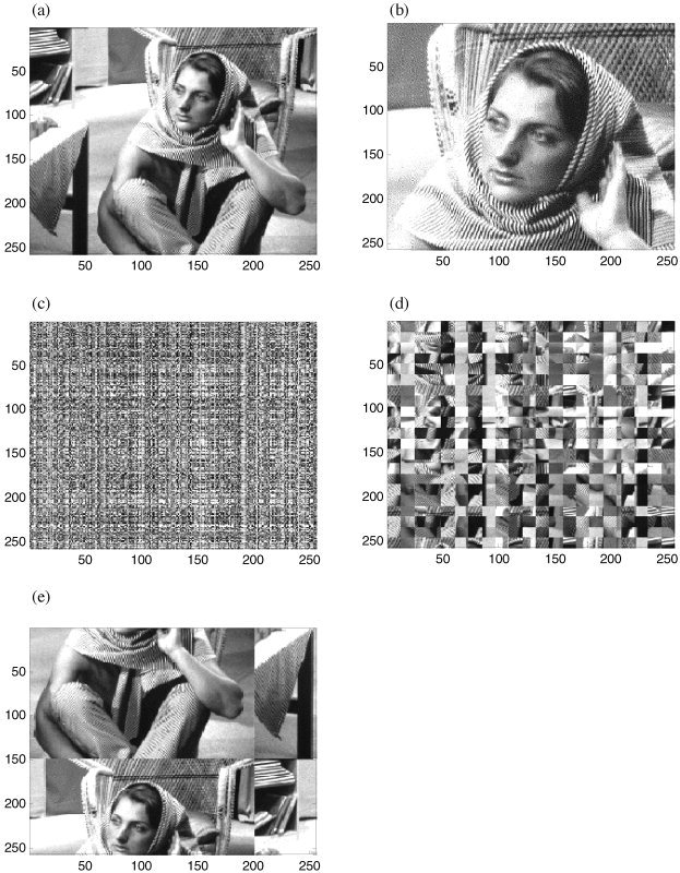
Standard test images used to illustrate the wavelet resampling scheme (a,b). Example of permutation schemes (operating on the raw image in a). c: Random permutation of rows and then columns. d: Resampling in 12 × 12 blocks. e: Cyclic rotation of rows and then columns.
Wavestrapping Within an Irregular Data Subdomain
It is possible to construct two‐dimensional surrogate data sets through randomization of the phases of a two‐dimensional Fourier series. However, the physiological component of many spatially extended biophysical data is confined to an irregular subdomain of the data. An example is the intracranial component of fMRI data. Hence, it is necessary to constrain the resampling technique so that the partition between the physiological and redundant data is retained. This is not possible with the Fourier technique, since the spatial localization of data is contained within the phases, which are randomized! However, because the detail coefficients of the wavelet transform are spatially localized, it is possible to achieve this using wavestrapping by only permuting coefficients that are located within the physiological domain (i.e., those with a non‐zero variance). Note that, because of edge effects of the wavelet functions, the set of coefficients belonging within the physiological domain is smaller than the set of non‐zero detail coefficients, even if the redundant data are zero. Detail coefficients outside of the physiological domain are left unchanged. Coefficients on the boundary of this domain (i.e., which may be partially centred on either side of the boundary) are included in the resampling scheme. Surrogate data are then obtained through inverse wavelet transform of the permuted and non‐permuted coefficients. It is important that the detail coefficients outside of the physiological domain are included in the reconstruction step because they contribute to the power of the voxels at the edge of the data set. However, they cannot be permuted because they naturally taper to zero as the support of the basis functions shifts further outside of the intracranial domain. This step is presented schematically in Figure 2.
Figure 2.
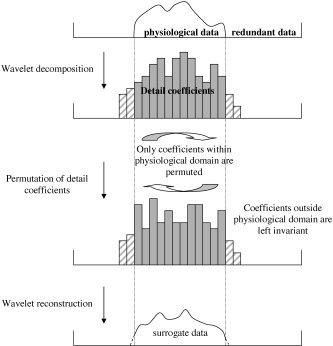
Schema illustrating how resampling is constrained to within physiological domain. The first step requires partition of the physiological domain from redundant data (with zero variance). After transforming the data into the wavelet domain, the coefficients that are located within, or on the boundary, of this domain are permuted amongst themselves. This procedure occurs on each level of the multi‐scale decomposition. Data are then reconstructed from the permuted coefficients within this domain and those outside it, which are left invariant. Any non‐zero data outside of the original physiological domain (dotted lines) at the end of the procedure are reset to zero. Hence, there is some loss of power, which can be rectified through renormalization.
Wavestrapping of Multiple Slices
Functional neuroimaging data consist of a temporal series of multiple slices. If surrogate data are constructed from each slice independently, then the spatial correlations between different slices and temporal correlations within a slice at different times will be destroyed. This problem can be overcome in multivariate one‐dimensional data by applying exactly the same permutation scheme to each data set [Prichard and Theiler, 1994]. Implementation of this technique in a variety of multivariate time series data reveals that, with appropriate choice of wavelet basis functions and resampling scheme, the correlation function can be closely preserved [Breakspear et al., 2003]. In the present study, the effect of generalizing this procedure to spatio‐temporal data is investigated. That is, a surrogate realization is generated by applying the same random permutation of detail coefficients to each two‐dimensional slice of interest, and to each decomposition obtained from a single slice across the temporal sequence of data collection.
Temporal Resampling
As with the spatial correlations, only the average and not the specific temporal correlations are required. To achieve this, a multivariate wavestrapping step must be performed in the temporal domain on the spatially resampled data. That is, a wavelet decomposition is performed on the time series of each intracranial voxel, the detail coefficients are permuted and surrogate data is obtained though the inverse wavelet transform. To ensure that the average spatial correlations, carefully preserved by prior steps, remain approximately the same as in the original data, the same permutation is performed on the decompositions from all voxels in the same and any other chosen slices. The effectiveness of this step is investigated by studying the temporal spectrum of whole slices' time series.
To summarize, the overall algorithm proceeds in two steps: Firstly a constrained spatial resampling and then a multivariate temporal resampling step (see Fig. 3). Because the wavelet coefficients are permuted throughout their length in the time domain, and throughout the entire intracranial domain, the presented technique is based upon an assumption of spatial and temporal “stationarity.” That is, the statistical properties of the data set under the null hypothesis are, on average, spatially and temporally invariant. Hence, the null hypothesis formally tested is that measures of functional connectivity derived from the data are due to background spatially‐invariant correlations arising from a stationary stochastic process. Rejection of this null hypothesis can thus be attributed to the presence of region‐specific (spatially variant) neural co‐activations and/or functional correlations. In certain circumstances, null rejection could alternatively be interpreted as evidence of dynamic or nonlinear correlations, which have been detected in scalp EEG [Breakspear and Terry, 2002b], MEG [Stam et al., 2003] and fMRI data [Friston et al., 2003; Harrison et al., 2003; Lahaye et al., 2003].
Figure 3.
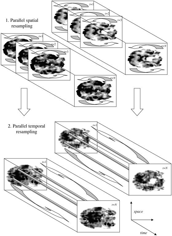
Schema of the two‐step resampling procedure. In step 1, each slice and at each time point is spatially resampled. The resampling procedure is identical at the same scale for each time point and each slice. Resampling at different scales is independent. In step 2, the time series from each voxel (three shown in each slice) from the spatially wavestrapped data is resampled in the temporal dimension. The resampling procedure at the same scale for each voxel is identical. All resampling is performed in the wavelet domain after appropriate wavelet decomposition (two‐dimensional for step 1 and one‐dimensional for step 2).
Spatial and Temporal Spectra
The spatial and temporal correlations and cross‐correlations of the data can be studied by plotting the spatial and temporal spectra. These are frequency‐specific representations of the corresponding correlation functions. Signals without memory (=no correlations) have flat spectra. Correlations introduce local and global features into the spectra. The temporal spectrum reflects correlated events occurring at different times; Spatial spectra (vertical and horizontal) capture correlations occurring at different regions in a spatial image or process. The usual meaning of a temporal spectrum is that derived from a single time series (such as from a pixel) using a one‐dimensional fast Fourier transform (FFT). However, it is also possible to take a 3‐D FFT of a complete slice's time series: Integrating in both spatial dimensions then yields the temporal spectrum for this slice. Integrating in time yields the average spatial spectra. Cross‐spectra are calculated from the cross‐products of the Fourier transforms of two slices. Because the integration is performed across the entire spatial/temporal domain, the assumption of spatiotemporal stationarity discussed above is also implicit in the derived spectra. Further discussion of temporal spectrum and spatial spectra and the corresponding formulae are given in Appendix B.
Choice of Basis Functions and Resampling Scheme
The surrogate data for the figures in this study were generated on a trial and error basis, the aim of which is to find the least constrained resampling scheme that yields an appropriate null distribution (a surrogate ensemble that adequately covers the experimental data with a reasonable variance). The following general principles were followed: Begin with a random permutation scheme and low order wavelet functions (such as Daubechies of order 2). The spatial and temporal (cross) spectra of the original and surrogate data are then plotted (see Figs. 9 and 10). The surrogate data are said to be adequate if the general underlying trend of the original data's spectra and those of the surrogate data are the same. If 19 surrogate data sets are constructed, then it is desirable to have approximately 5% of the spectra samples outside of the surrogate distribution. If the spectra are not adequate (such as due to whitening of the surrogate data at high frequencies), the order of the wavelet functions is iteratively increased. However, once Daubechies wavelets of order 12 or more are employed, a low‐frequency bias of the surrogate spectra (typically an isolated trough at low frequencies) often appears. These are due to increased edge effects arising as the length of the wavelet functions' support increases. It is hence necessary to choose the highest order functions at which this is not observed. If the surrogate spectra are still not adequate, then it is necessary to move from a random resampling scheme to block resampling, iteratively increasing the size of blocks from 2 to N j/3. If the surrogate spectra are still inadequate, it is necessary to change to a cyclic rotation of the detail coefficients. These principles are outlined schematically in Figure 4.
Figure 9.
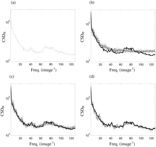
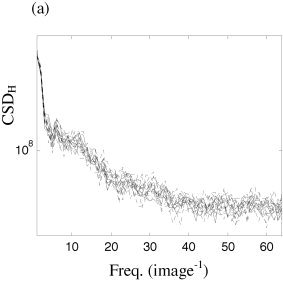
a: Horizontal spatial cross‐spectrum the images in Figure 1a,b. Corresponding cross‐spectra (b) of an ensemble of 19 surrogate sets produced by random permutation of detail coefficients. Cross‐spectra produced by (c) resampling in blocks of 12 adjacent coefficients and (d) cyclic rotation of detail coefficients.
Figure 10.
a: Horizontal spatial spectrum of a motion‐corrected fMRI slice. Spatial spectra produced by resampling wavelet coefficients using (b) Daubechies wavelets of order 4 and (c) order 6
Figure 4.
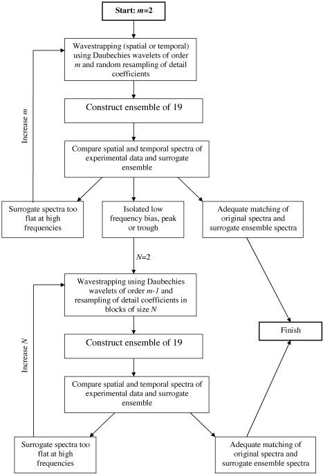
General principles followed to choose wavelet basis functions and resampling scheme. Procedure commences with random resampling and wavelet basis functions of low order, m = 2. This order is increased until there is an adequate matching of the spectra (→ finish) or isolated bias in the spectra appear (due to edge of effects of high order basis functions). If this occurs, m is reset to m‐1 and the coefficients are resampled in small blocks of N = 2. The size of the blocks is increased (N→N+1) until there is an adequate matching the spectra. If N approaches half of the length of the number of coefficients, then cyclic rotation is employed.
Subjects and fMRI Data Acquisition
Data set 1: visual activation data
Participants were eight healthy male volunteers (mean age 31 years). Exclusion criteria were left‐handedness, and recent history of substance abuse, epilepsy, or other neurological disorders, and mental retardation or head injury (assessed using the Westmead Hospital Clinical Information Base questionnaire; WHCIB). Written consent was obtained from all subjects prior to testing in accordance with National Health and Medical Research Council guidelines. To produce visual sensory stimulation, we used a periodic presentation of checkerboard (test) and blank screen (control) stimuli. Four test stimulus blocks alternated with four control blocks. Stimuli were 512 pixels in height, and 384 in width, with 20% contrast. On checkerboard stimuli, checks were coloured blue and green. In test blocks, the checkerboard pattern was reversed in an alternating sequence (i.e., green checks appeared blue, and vice versa on every second checkerboard stimulus). Each block comprised eight stimuli of 3‐sec duration, with an interstimulus interval of 0.75 sec. The duration of each block was, therefore, 30 sec. There were 32 test and 32 control stimuli in total, and the total duration of the paradigm was 4 min [Williams et al., 2000]. Subjects were scanned during the checkerboard task using a Siemens 1.5 T Magnetom VISION Plus system to acquire 64 T2‐weighted images depicting BOLD (blood oxygenation level dependent) contrast for each 3‐sec stimulus at 18 axial non‐continuous 6‐mm‐thick plane (slices), parallel to the intercommissural (ACPC) line: time to echo (TE) 40 msec, TR 3 sec with 0.75‐sec delay, matrix 128 × 128, interslice gap 0.6 mm at Westmead Hospital, Sydney.
Data set 2: resting or “null” data
Three healthy volunteers were studied while they lay quietly in the scanner with their eyes closed for 5 min. One hundred T2‐weighted images were acquired at each of 14 non‐contiguous slices of data in an oblique axial plane using the 1.5 Tesla (T) GE Signa system (General Electric, Milwaukee, WI) at the Maudsley Hospital, London, UK: TE 40 msec, TR 3 sec, in‐plane resolution 3 mm, slice thickness 7.7 mm, number of excitations 1.
Processing of fMRI Data
Prior to analysis, all images were first pre‐processed to minimize the effects of subject motion [Bullmore et al., 1999]. The effect of the underlying anatomical signal was addressed by subtracting the temporal mean from each individual pixel's time series. Neural activation in the visual stimulation data was determined according to the nonparametric method described in Brammer et al., [1997]. The patterns of activation in this data set have been previously reported elsewhere [Williams et al., 2000]. The wavestrapping was applied to the underlying (temporally de‐meaned) BOLD signal, not the “residuals” of the nonparametric model. The technique used to identify areas of activation in the visual stimulation data [Brammer et al., 1997] requires spatial filtering by convolution with a Gaussian curve (FWHM = 9.4 mm, kernel = 9 × 9 pixels). Whilst it would be possible to construct surrogate data from the spatially filtered data, it is preferable to use the raw images. The surrogate data are subsequently subject to the same spatial filtering as the experimental data.
Illustration and Validation in Nonphysiological Data
To illustrate the method visually, and to validate it in data with varying spatial correlations, the algorithm is applied to two standard IEEE test images, presented in Figure 1a and b. These are chosen because the spatial correlations can be visualized across a hierarchy of scales and localized to specific spatial locations (for example, fine structure within the lattice of the chair and the scarf, coarse structure of the shadows). Appropriately resampled data should retain the correlations but randomize and/or disperse their spatial localization. The test images are more suitable than physiological data to allow visualization of this effect.
RESULTS
Illustration on “Test Image”
The effect of wavestrapping in the spatial domain at different scales is illustrated in Figure 5. Horizontal, vertical and diagonal coefficients were permuted together. In Figure 5a, only the finest details have been resampled. In comparison to Figure 1a, it is evident that the fine detail of the scarf and the chair lattice has been moved. However, this structure has not been smoothed out of the picture, but is evident diffusely through the background of the entire frame. The number of scales on which the resampling operates has been increased to 2 (Fig. 5b), 3 (Fig. 5c), 4 (Fig. 5d), and all scales (Fig. 5e). Varying the scales at which the permutation acts makes evident the manner in which the structure at each scale contributes to the information in the image. For example, in Figure 5d, only the coarsest shadows of the face remain in their original location. Structure at all smaller scales is now present diffusely throughout the image. This bears out the difference between the particular correlations in an image, which impart crucial information and background structure that is typical of the data set, which is still present in all panels of Figure 5. In Figure 5f, the structure at the three smallest scales has not been resampled. Hence, the facial features and scarf pattern remain in their original spatial location. However, the shadows, which give the image its depth, are now present diffusely throughout the image. In this image, specific information at various scales conveys certain types of information (detail, depth, texture, etc). In neuroimaging data, it is expected that fluctuations in neural activity at different scales signify different types of neural interactions and information processing.
Figure 5.
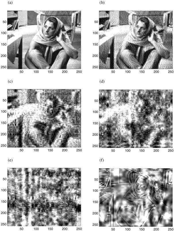
Effect of resampling in the wavelet domain at different spatial scales. a: Scale 1 only. b: Scales 1–2. c: Scales 1–3. d: Scales 1–4. e: Scales 1–8 (effectively all scales). f: Scales 4–8. Daubechies wavelets of order 12 were used.
In Figure 6, the effect of constraining the resampling of coefficients to a subdomain of the data set is illustrated. The resampling has been restricted to an ellipse (horizontal radius 70 pixels, vertical axis 100 pixels). It can be seen that the spatial correlations within this ellipse have been randomised, whereas those outside have been unchanged. Slight blurring at the edge of the ellipse, due to edge effects of the wavelet functions, is evident.
Figure 6.
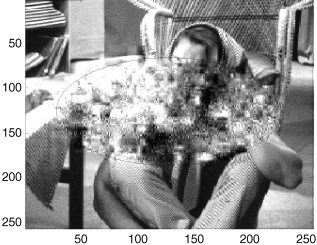
Restriction of resampling of detail coefficients to within a central ellipse with a horizontal axis of 200 voxels and a vertical axis of 140 voxels. Coefficients outside this sphere were not permuted. Black (superimposed) curves show extent of sphere.
Effect on Spatial Spectra of “Test Data”
Power spectra of single image surrogates
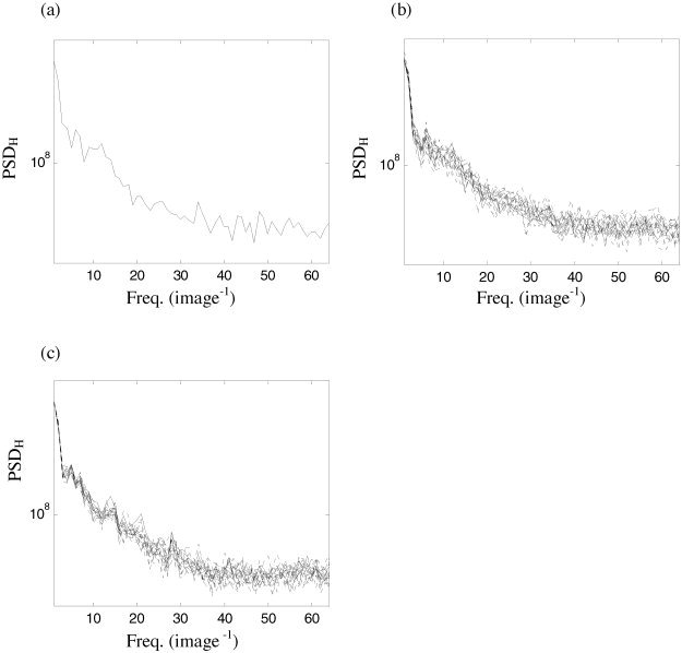
In order to verify that the spatial wavestrapping does not whiten the data, it is necessary to study the horizontal and vertical spatial spectra. Adequate preservation of the linear correlations is verified if the spectrum of the original data is contained within the spectrum of an ensemble of surrogate data. In this section, the results of permutation of all detail scales are presented. The results are illustrated in Figure 7 (for brevity, only horizontal spectra are shown in all figures; results for vertical spectra are always comparable).
Figure 7.
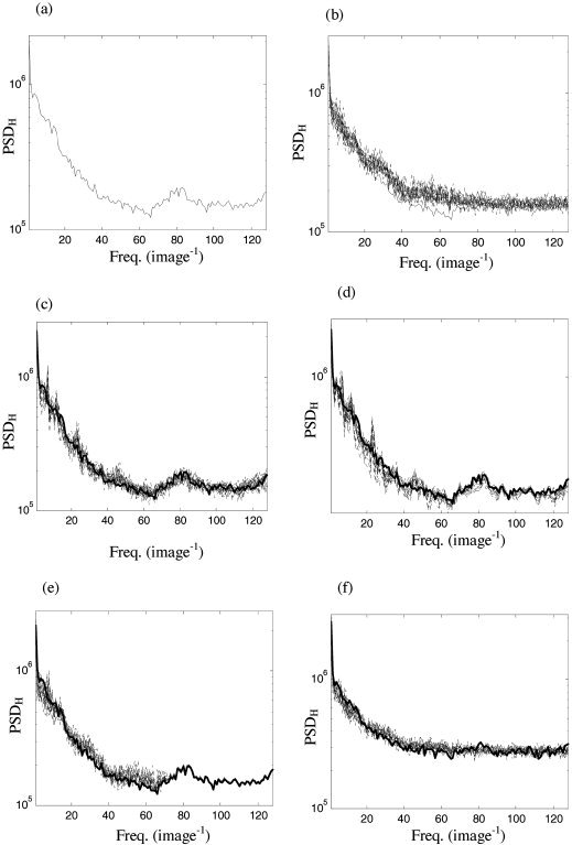
a: Horizontal spatial spectrum of the image in Figure 1a. b: Corresponding horizontal spectra of an ensemble of 19 surrogate sets produced by random permutation of detail coefficients. c: Horizontal spectra produced by resampling in blocks of 12 adjacent detail coefficients. d: Horizontal spectra produced by cyclic rotation of detail coefficients. e: Horizontal spectra produced after restricting random permutation of detail coefficients to all scales other then the finest. f: Horizontal spectra produced by random permutation of coefficients (a) plus additive Gaussian noise. For all panels, Daubechies wavelets of order 12 were employed.
The horizontal (PSDH) spatial spectra of the image in Figure 1a are presented in Figure 7a. In Figure 7b, the original (heavy) and ensemble of 19 surrogate data (light) produced by random permutation of detail coefficients are illustrated. It can be seen that, although the overall trend is preserved, there is some loss of the detailed peaks and troughs, and some whitening of the high‐frequency end of spectrum. In contrast, resampling of detail coefficients in blocks of 12 adjacent coefficients (Fig. 7c) ensures that the spectra of the original image are almost completely within the surrogate ensemble. Note that as 19 surrogate sets were generated for this Figure 7, 5% of the original spectral values are permitted to lie outside of the surrogate ensemble. Cyclic rotation of detail coefficients (Fig. 7d) produces surrogate data with a very close spectral match to the original data and less variance than produced by block resampling.
The proximity of the surrogate data spectra to the original spectra is apparent visually. Example surrogate images from each of the three schemes are presented in Figure 8. The random permutation scheme (Fig. 8a) produces an image in which the structure at various scales is scattered diffusely throughout the image. In contrast, if there was some “clustering” of the structure in the original image (such as the pattern on the scarf), then to some extent that clustering is preserved in the surrogate produced by block resampling (Fig. 8b) and cyclic rotation (Fig. 8c). This additional retention of structure accounts for the preservation of the peaks with these resampling schemes' spectra.
Figure 8.

Visual representation of spatial wavestrapping at all spatial scales. a: Random permutation; b: Resampling in blocks of 10x10 coefficients; c: Cyclic resampling.
Further constraining the resampling to within only a few levels or within only a subdomain of the data can only lead, on average, to an improvement in the match of the spectra. This is because the range of possible permutations of the constrained resampling is a subset of the original possibilities (in group theoretical terms, the set of possible group elements is a subgroup of the chosen scheme), and hence the distribution of possible spectra is contained within the broader unconstrained distribution. This is illustrated in Figure 7e where surrogate data have been produced by random permutation of all detail coefficients except those at the finest scale. Note that in contrast to Figure 7b there is now almost perfect matching of the spectrum at high frequencies.
The success or failure of the resampling scheme depends upon the strength of the spatial correlations within the data. Typically, in an experimental setting, the data will be corrupted by measurement noise. To simulate this, a Gaussian signal with average amplitude 40% of the original data was added to the image in Figure 1a. The resulting spectra obtained with random permutation of detail coefficients are presented in Figure 7f. Note that the original spectra are now flatter and less detailed, and that there is now adequate matching of the surrogate spectra.
The permutation of the horizontal, vertical, and diagonal detail coefficients together, as was performed for Figure 5, or independently has negligible effect on the closeness of fit between the spectra of the original and surrogate data. In many cases, it is possible to permute them independently. However, occasionally the situation arises when the slight extra advantage of parallel permutation is required.
Cross‐spectra of multiple images
In order to test the effect of the multi‐slice spatial resampling technique on correlations between the two test visual images (Fig. 1a and b), we study the spatial cross‐spectra (only the horizontal are plotted). The formulae for these are given in Appendix B.
The horizontal (CSDH) spatial cross‐spectrum of the images in Figure 1a and b is presented in Figure 9a. In Figure 9b, the original (heavy) and ensemble of 19 surrogate data (light) produced by random permutation of detail coefficients are illustrated. It can be seen that the results, in terms of the preservation of the cross‐spectra, are comparable to that of the spectra of a single slice. Likewise, there is substantial improvement when moving to multi‐slice block resampling (Fig. 9c) and cyclic resampling (Fig. 9d). Hence, as with the one‐dimensional surrogate data schemes, wavestrapping of two‐dimensional data sets can be generalized in order to preserve cross‐correlations between multiple data sets (such as adjacent slices in the third spatial dimension).
Application to fMRI Data
From the preceding analysis, and given that fMRI data sets are relatively small in size, it is expected that the wavestrapping algorithm may only adequately preserve the spatial and temporal spectra if the correlations (steepness of the power spectral curves) are relatively weak. Hence, the adequacy of the proposed technique for fMRI data is an empirical issue and cannot be determined a priori. The results are presented in this section.
Spatial wavestrapping step
In the present data set, the spatial correlations are comparatively weak. In Figure 10a, the horizontal spatial spectrum of one typical slice from the visual activation data set is presented. In Figure 10b, this spectra is plotted alongside 19 surrogate realizations (dashed lines) from the spatial wavestrapping step. The results of resampling another (randomly chosen) slice, from a different subject, are presented in Figure 10c. As discussed in Bullmore et al. [2001], higher‐order wavelet basis functions more completely decorrelate the detail coefficients than low‐order wavelets. However, due to the relatively featureless nature of the spatial spectra, adequate results were obtained with relatively low‐order wavelets Here, wavelets of order 4 (Fig. 10b) and 6 (Fig. 10c) were used.
It is also necessary to scale up the power of the surrogates by about 10% to match the original data. This is because power within the centre of the image will be permuted close to the boundary. Some of this power will then be spread outside of the boundaries during the inverse DWT and hence lost from the image. However, this can easily be rectified by automated renormalization of the data and does not introduce any further problems, as evidenced by the appropriate matching of the spatial spectra of the original and (renormalized) surrogate data in Figure 10.
Sample images were studied in each subject. Although, for most subjects, isolated peaks in the spectra and cross‐spectra (i.e., local minima or maxima in the power‐frequency plots such as in Fig. 10c) may not have been contained within the surrogate distribution, we were able to easily locate suitable wavelet basis functions for all slices studied. On no occasions did there exist unrectifiable whitening or distortion of the spectra. As discussed above, with 19 surrogate sets, it is adequate to have only 95% or the surrogate spectra data points within the null distribution and this was always attainable.
The horizontal spatial cross‐spectrum between two adjacent images in one subject is presented in Figure 11. Daubechies wavelets of order 6 were employed to generate surrogate data. It can be seen that the cross‐spectra of the original data are contained within the null distribution. This step does generally require slightly higher‐order wavelet basis functions.
Figure 11.
The horizontal spatial cross‐spectrum between two adjacent slices in one subject (solid line) and cross‐spectra produced by resampling coefficients using a Daubechies wavelet of order 6 (dashed line).
What effect does the “parallel” spatial wavestrapping step have on the temporal spectrum of an entire slice's time series? An example of a temporal spectrum of a slice from the “resting” fMRI data set and 19 surrogate data sets constructed from spatial wavestrapping with Daubechies wavelets of order 6 is given is Figure 12a. It can be seen that although the match is not exact, the variance of the surrogate data is very small.
Figure 12.
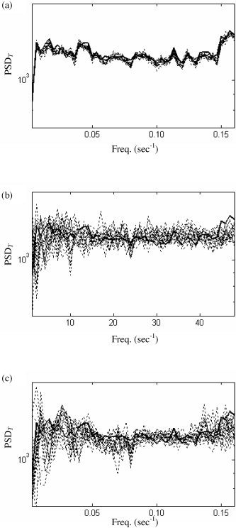
Temporal spectrum (PSDT) of original data (solid line) and surrogate data (dashed line). (a:) PSDT following parallel spatial resampling using Daubechies wavelets of order 6. b,c: The effect of subsequent temporal resampling on these spatially wavestrapped data, using (b) Daubechies wavelets of order 8 in 5 blocks and (c) Daubechies wavelets of order 10 and random permutation. Note the increase in variance in b and c.
Combined spatio‐temporal wavestrapping steps
In Figure 12b,c, the effect on the temporal spectrum of adding on the temporal wavestrapping step is studied. Each surrogate has been generated through temporal wavestrapping one of the spatially wavestrapped surrogates in Figure 12a. Figure 12b was produced using Daubechies wavelets of order 8 resampled in 5 blocks. Figure 12c employs random permutation after decomposition with Daubechies wavelets of order 10. Figure 12 (b and c) shows that although the original spectrum remains appropriately contained within the surrogate ensemble, the variance has greatly increased. This can be formalised by calculating the average root‐mean‐square deviation of each surrogate spectrum from the spectrum of the original data. In Figure 12a, the mean rms deviation is 37 units. In Figure 12b and c, it has increased to 129 and 125 units, respectively. This is an important effect because if the variance is too small, then the surrogate ensemble does not adequately represent a null distribution [Kugiumtzis, 1999]: An insufficient variance around the original data increases the rate of false‐positive rejections of the null hypothesis. This is discussed further below.
The spatial and temporal steps can be reversed: This permits investigation of the effect of “parallel” temporal resampling on the spatial spectra of each image (which we claimed should also be closely preserved). The results are presented in Figure 13. An example of spatial spectra of a slice from the “resting” fMRI data set and 19 surrogate data sets constructed from temporal wavestrapping with Daubechies wavelets of order 10 are given in Figure 13a. Although the spatial spectra are not preserved as closely as the temporal spectrum following parallel spatial resampling (Fig. 12a), there is still an appropriately good fit. The mean rms difference between the original and surrogate spectra is 97 units for the horizontal and 112 for the vertical spectra. The effect of adding on spatial resampling using Daubechies wavelets of order 6 (Fig. 12b) and 8 (Fig. 12c) is to increase the variance and hence smooth out the close matching of local peaks in the spectra: The rms differences have increased to 132 and 146 units for the horizontal and vertical spatial spectra for both rows of spectra. Hence, the effect and import of the parallel temporal resampling step are comparable (although less pronounced) to parallel spatial resampling.
Figure 13.
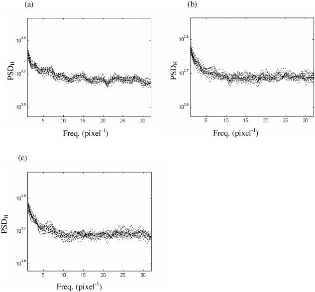
Horizontal (PSDH) spatial spectra of the original data (solid line) and surrogate (dashed line). a: Spatial spectra following parallel temporal resampling with Daubechies wavelets of order 10. Subsequent spatial resampling on these temporally wavestrapped data, using Daubechies wavelets of order 6 (b) and 8 (c).
It is also important to determine whether the variability of the surrogate realizations in the voxels at the edges of the brain is suitably high, and not unduly constrained by the lack of resampling of the detail coefficients in the adjacent extracranial space. This was investigated by measuring, in each voxel, the root‐mean‐square difference between the time series of each surrogate realization and the original data. The mean value of this difference over all surrogates reflects the degree of variability of surrogate realizations, voxel by voxel. Results are plotted in Figure 14. In Figure 14a, a typical cross‐section of this measure across the brain is plotted. The dashed line is derived from spatially resampled data and the solid line after spatiotemporal resampling. In Figure 14b, a grey‐scale image of an entire slice after spatiotemporal resampling is given. The notable feature of both plots is that the edges are steep, indicating that any reduced variability affects very few voxels. In Figure 14a, it can be seen that there is some reduced variability, but only for a few (one to three) voxels at the edge of the data. This is because at the finest scale of the wavelet decomposition, the basis functions have very small support and hence still ensure adequate mixing at the edges of the permuted data set (leaving the finest level unpermuted yields spatially resampled data with flatter edges). The temporal resampling step redresses any incomplete resampling that does occur at the edges. Nonetheless, care should be taken if dealing with very superficial cortex using the present approach.
Figure 14.
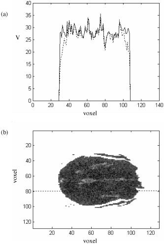
Mean of the root‐mean‐square of the difference between the experimental BOLD and surrogate time series, voxel by voxel. a: Cross‐section through a slice, showing results after spatial wavestrapping (dashed line) and spatiotemporal wavestrapping (solid line). Note somewhat steeper “edges” after both steps have been completed. b: Grey‐scale results from an entire image. Dotted line shows location of the cross‐section in a.
The amplitude distribution of a single slice fMRI (throughout the recording) and two sample surrogate sets are given in Figure 15. The BOLD value in each pixel at all time points was extracted and the resulting values are plotted on an amplitude histogram. An original data set is given in black. Note that the distribution is approximately Gaussian. The amplitude distribution of a surrogate set derived by spatial wave‐strapping is given in light grey. The distribution of a surrogate set derived by spatial and temporal wave‐strapping is given in dark grey. It can be seen that the wave‐strapping algorithm has a negligible effect on the amplitude distribution. Given that the amplitude distribution of the fMRI data is effectively Gaussian, this finding is not surprising: both the phase‐randomizing [Theiler et al., 1992] and wavestrapping [Breakspear et al., 2003] techniques tend to bias any data toward a Gaussian distribution. Other issues related to wavestrapping of one‐dimensional uni‐ and multivariate data sets have been examined in more detail elsewhere [Andrzejak et al., 2004; Breakspear et al., 2003; Bullmore et al., 2001].
Figure 15.
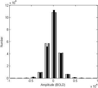
Amplitude histogram of fMRI data (black), spatially wave‐strapped data (light gray) and spatio‐temporal wavestrapped data (dark grey). The BOLD value in each pixel at all time points was extracted and the resulting values are plotted on an amplitude histogram. x‐axis is the value of the BOLD signal and the y‐axis gives the number of voxels with that signal value.
Analysis of “null” data set
The validity of the spatiotemporal wavestrapping technique can be studied by comparing the expected versus observed rate of null hypothesis rejections using a measure of functional connectivity in the “null” (resting) fMRI data sets. For the present study, we employed the Pearson's correlation coefficient r, a simple measure of linear correlation/co‐activation. In each data set, 1,000 distinct randomly chosen pairs of voxels were studied. For each pair, a one‐tailed test of significance was performed by comparing the experimentally derived correlation coefficient r exp against the rank ordered measures derived from 19 sets of surrogate data r surr. The null hypothesis was rejected if r exp > max (r surr).
The results for the overall analysis in the 3 “null” data sets are presented in Figure 16. Figure 16a shows results from one slice in the first subject using a number of resampling strategies. Following spatial resampling alone (dashed line/crosses), it can be seen that the observed number of null rejections very closely mirrors the expected number. Results from four different subsequent temporal resampling strategies are shown with dotted lines. It can be seen that all give valid although slightly conservative results over a wide range of P values. Random recycling with Daubechies wavelets of order 10 (black dots) most closely matches the expected rate of false positives. In this example, permuting detail coefficients in 4 blocks using wavelets of order 8 (Fig. 16, diamonds) yielded the most conservative outcome. In Figure 16b and c, results from the two other data sets are given. In these subjects, two slices were processed and one voxel from each slice was included in each randomly chosen pair. In these slices, the temporal resampling step was performed first (dotted lines/circles) using Daubechies wavelets of order 6. In Figure 16a–c, results from three spatiotemporal surrogates constructed by subsequent spatial resampling with Daubechies wavelets of order 4 to 10 are given (dashed lines). The results are comparable to Figure 16a with the exception that the temporal resampling step in subject 2 (dotted line in Fig. 16b) gives a somewhat more conservative output than the first step in Figure 16a. However, it is clear that in all subjects, suitably valid representations of the null hypothesis were generated following a variety of resampling choices.
Figure 16.
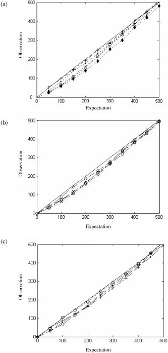
Expected versus observed rate of null hypothesis rejection in the eyes‐closed resting state fMRI data set. a: Results following first subject, one slice after spatial wavestrapping using daubechies wavelets of order 6 (crosses, dashed line) and then subsequent temporal resampling (dotted lines) using wavelets of order 10 and random resampling (black dots), 8 and cyclic rotation (crosses), 8 and random resampling (open circles), 8 and resampling in 4 blocks (diamonds). Results from second (b) and third (c) subjects showing temporal resampling (dotted line) using Daubechies wavelets of order 6, and then spatial resampling using wavelets of order 4 (crosses), 6 (diamonds), and 8 (black dots).
Results from visual activation paradigm
It is reasonable to expect that activity arising from co‐activation of bilateral visual cortex following visual stimulus (first data set) should exhibit region‐specific correlations. If so, then the wavestrapping algorithm should randomise such effects into the background structure. We identified those data sets where strong activation was observed to occur in visual cortex and compared the correlation coefficient from the experimental data with ensembles of surrogate data. Daubechies wavelets of order 3 to 8 were employed, according to the schema outlined in Figure 3. Two slices from each subject were studied. An example of this analysis is presented in Figure 17. Figure 17a and b show the BOLD time series for two strongly activated voxels and their corresponding spatiotemporal surrogates. The temporal cross‐spectrum of the two voxels is given in Figure 17c. It can be seen that the cross‐spectrum of the original data is outside of the surrogate distribution: The null hypothesis can be rejected for these voxels (r exp = 0.794; max(r surr) = 0.717, mean(r surr = 0.629).
Figure 17.
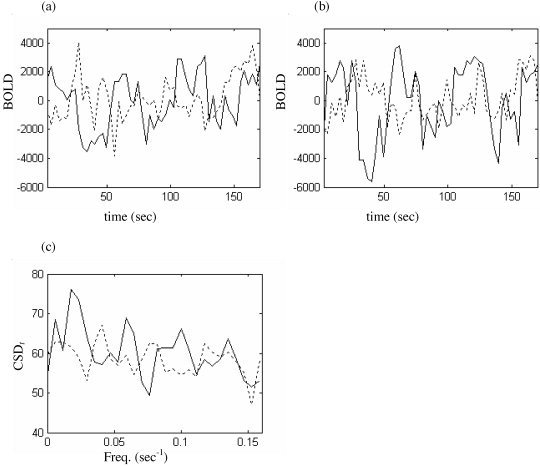
Exemplar data from visual stimulation paradigm. a,b: Time series of BOLD from two “strongly activated” pixels in visual cortex (solid line) and corresponding surrogate realizations (dashed line). c: Corresponding temporal cross‐spectral density function. Pearson's correlation coefficient for the original data was r exp = 0.794 and for the surrogate r surr = 0.637 (the median for this surrogate ensemble).
The overall results are presented in Table 1. Seven suitable data sets were identified. As shown in the second column in Table I, the experimental correlation coefficients were all reasonably strong. As expected, all of these were statistically significant following one‐tailed nonparametric comparison with surrogate values (i.e., r exp > max(r surr)). Thus, the wavestrapping algorithm did appear to achieve adequate randomisation of such expected effects. In the third column (Table I), the mean values of r surr are shown. It can be seen that, whilst weaker than the corresponding experimental values, all means except one are much stronger than zero. This is not surprising, given the relative proximity of the pairs of voxels in this strongly stimulus‐driven data set. Further analysis, possibly using simulated data, would be required to ensure that the background correlations were adequately randomised from such data.
Table I.
Pearson's correlation coefficient from experimental and spatiotemporal surrogate ensembles in six subjects (where strong activation was observed in bilateral visual cortex) of the visual stimulus data set
| Subject | r exp | r surr | ||
|---|---|---|---|---|
| Max | Mean | Min | ||
| nc1 | 0.688 | 0.608 | 0.413 | 0.106 |
| nc2 | 0.604 | 0.564 | 0.335 | −0.097 |
| nc5 | 0.442 | 0.401 | 0.263 | 0.013 |
| nc7 | 0.616 | 0.567 | 0.416 | −0.156 |
| nc15 | 0.665 | 0.558 | 0.379 | 0.127 |
| nc16 | 0.794 | 0.717 | 0.629 | 0.397 |
| nc17 | 0.550 | 0.384 | −0.022 | −0.423 |
* Experimental r exp versus surrogate r surr values. A one‐tailed non‐parametric rejection of the null hypothesis is said to occur if r exp > max(r surr).
DISCUSSION
In this report, we present a wavelet‐based method of constructing surrogate data for null hypothesis testing in functional connectivity studies. The method is an extension of previous “wavestrapping” algorithms from a one‐dimensional univariate [Bullmore et al., 2001] and multivariate [Breakspear et al., 2003] data to spatio‐temporal data with an irregular physiological subdomain. Using standard IEEE test images, the effects of different constraints on the resampling procedure were visualized in the real and spectral domains. It was hence shown that the algorithm could be tailored to suit data sets with different spectral properties, and constrained to within various spatial scales and spatial subdomains. Correlations within and between slices in the spatial and temporal domains were observed to be adequately preserved.
It was demonstrated that the algorithm is suitable for use in a set of human fMRI data recorded during a visual stimulation paradigm. This requires restricting the resampling scheme to an irregular intracranial domain, a step that cannot be achieved with Fourier‐based resampling schemes. The only other surrogate data alternative that we are aware of is associated with a heavy computational burden in one‐dimensional data [Schreiber, 1998]. Given that computational demands increase approximately to the power of the number of dimensions, the proposed algorithm currently stands as the only viable non‐parametric method of estimating the null distribution for functional correlations in fMRI data. Moreover, its flexibility means that if non‐neural components of the data (such as cardiorespiratory effects) are restricted to within temporal or spatial subscales, they can be left “unpermuted.” In this way such effects will be present in the surrogate data in the same way as in the original data, and there will thus exist implicit control for their bias of any connectivity measures.
However, there are a number of important potential limitations of the method, which must be kept in mind when interpreting its application. The first of these is the impact of the algorithm on the amplitude distribution of the data. That is, the amplitude distribution of the surrogate data is not necessarily the same as that of the original data. This is also true of Fourier‐based techniques. This may lead to false rejections of the null hypothesis (type I errors). There are a number of solutions to these problems. (1) If the change in amplitude is only modest (see Fig. 14), then no action may be required. (2) A “goodness of fit” criteria of the amplitude distribution can be calculated [Breakspear et al., 2003] and surrogate data realizations discarded if they do not meet this criteria. (3) An “amplitude adjustment step” [Theiler et al., 1994] can be added to the algorithm [Breakspear et al., 2003]. However, whilst it is fairly straightforward to implement, such a step has its own limitations [Kugiumtzis 1999; Schreiber and Schmitz, 1996]. (4) The correlation measure can be checked to see if it is influenced by changes in the amplitude distribution without distortion of the spectra. This is often the case.
Secondly, in the present fMRI data, the temporal and spatial correlations were reasonably weak (see Figs. 12, 13). However, if such correlations were stronger, it might not be possible to adequately match the spectrum. At this stage, this can only be determined on an empirical basis. However, we did not find any data that could not be adequately resampled by this wavestrapping scheme.
Thirdly, the spatial resampling step in this report is a multivariate two‐dimensional algorithm. This is ideally suited to correlation measures within one or between two fMRI slices. However, some methods (such as PCA) incorporate multiple slices. Whilst it is possible to use the proposed method in this context, the correlations between slices are very closely preserved. This may lead to a slightly over‐conservative estimation of the null hypothesis (hence type II errors). This arises because the wavelet decomposition is only two‐dimensional. In order to preserve only the average between slice correlations (which are dependent on the separation distance between multiple slices), a full three‐dimensional wavelet decomposition would be required. This is to be the subject of future work.
Fourthly, the effects of the boundaries (the spatial and temporal endpoints) of the data may be a potential problem [Rapp et al., 2001], particularly if high‐order wavelet functions (which have a wider support and hence spread further over the boundaries) are employed. However, in the spatial domain, at least in our data, this was not found to be a problem because there existed a significant number of redundant data points outside of the intracranial domain. These act to “pad” the effect of the outer boundaries of the data and hence greatly diminish boundary effects. Thus, we did not observe significant spectral distortions even with relatively high‐order wavelets.
Fifthly, although the method was validated in a “null data set,” it is important to bear in mind that this assumes that there are only randomly distributed (null) linear correlations in fMRI signal intensity during resting (eyes closed) cognitive states. A number of recent studies have, on the contrary, reported evidence of specific and distinct patterns of functional connectivity in resting states, involving primary motor [Xiong et al., 1999] and visual cortex [Lowe et al., 1998], left and right hippocampus [Rombouts et al., 2003], and the cingulate cortex [Grecius et al., 2003]. Such effects may be comparable to the temporally sparse occurrence of dynamic connectivity in resting state scalp EEG [Breakspear and Terry, 2002b] and have been posited to support the retrieval and manipulation of episodic memories [Grecius et al., 2003]. To some extent, the relative sparsity of such regions, combined with the random choice of pairs scattered over the entire cortex, should partially overcome such effects for the present purpose. Further empirical study of resting state neuroimaging data is required to better survey the extent, sparsity, and strength of such functionally connected networks. Spatiotemporal wavestrapping could play an important role in such an endeavour.
When dealing with moderately large data sets, computational considerations are also important. Using Daubechies wavelets of order 8 in MatLab 6.5, the spatial wavestrapping step takes approximately 30 sec for one slice with 55 time points on a Pentium IV 1.6GHz processor. The multivariate temporal wavestrapping step takes approximately 130 sec. Hence, for two slices in one subject, construction of a 19‐sample surrogate ensemble takes approximately 2 h. Computation times decrease when lower order wavelet functions can be employed and would be lower still if the algorithms were compiled in “lower level” languages such as C. Once constructed, the surrogate data could be employed to test a range of “connectivity” hypotheses. These considerations argue that the proposed technique is computationally feasible.
Finally, there is an important conceptual question: How much of the spectrum should be preserved? The closer the surrogate spectra to the original spectrum, the fewer the number of possible surrogate realizations. For example, the “size” (number of elements) of symmetry groups is orders of magnitude greater than that of cyclic groups. It is possible that many of the latter realizations, whilst closely matching the spatio‐temporal spectra, actually too closely resemble particular properties of the original data. This may cause type II errors (because the surrogate data have too much structure to sufficiently represent the null hypothesis). Alternatively, they may too closely resemble each other, that is, lack sufficient statistical independence [Dolan and Spano, 2001; Kugiumtzis, 1999]. This may allow type I errors (because the confidence interval is too narrow). Hence, when choosing the optimal wavelet basis functions and resampling scheme, it is desirable to find the wavestrapping scheme that generates the broadest surrogate distribution around the original data. For this reason, cyclic rotations of high‐order wavelet decompositions should not be the scheme of first choice.
Hence, interpretation of results using surrogate data needs to be conducted with caution. However, if these caveats are adequately accounted for, the present method remains a powerful non‐parametric method for use in studies of connectivity in functional neuroimaging data. An important future development would be to automate the selection of wavelet basis functions and resampling scheme illustrated in Figure 4. Because of the considerations discussed above, one desires the scheme that generates the broadest variance in the resampled ensemble spectra but that also adequately encloses the experimental spectra. It may be possible to minimise the number of iterations required to find the best scheme/basis functions by employing a searching algorithm such as simulated annealing. An alternative approach, not addressed in the present study, would be to characterize the nature of the stochastic process underlying the data's spatial and temporal spectra: Fractional Brownian motion [Bullmore et al., 2001] and autoregressive noise [Harrison et al., 2003] are two possible candidates. Wavelet functions of appropriate order and support could then be chosen after parameterizing the noise process. Such a study, which would require further analytic results on the decorrelating properties of higher‐order wavelets and an improved characterization of the spatio‐temporal stochastic structure of fMRI data, is to be the subject of future work.
Supporting information
This article contains supplementary material, in the form of visual animations of original and wave‐strapped surrogate data, which can be found online at http://www.interscience.wiley.com/jpages/1065-9471/suppmat
Supporting Information file suppmat_1957.pdf
Supporting Information file suppmat_1957_movie1.avi
Supporting Information file suppmat_1957_movie2.avi
Supporting Information file suppmat_1957_movie3.avi
Supporting Information file suppmat_1957_movie4.avi
Acknowledgements
M.J.B. was a recipient of a NSW Institute of Psychiatry Research Fellowship, a University of Sydney SESQUI post‐doctoral fellowship, and a Pfizer Neuroscience Research Grant. This Human Brain Project/Neuroinformatics research was also supported by the National Institute of Biomedical Imaging and Bioengineering and the National Institute of Mental Health. P.D. acknowledges the support of the Neuroscience Institute of Schizophrenia and Allied Disorders. The authors acknowledge the invaluable suggestions by two anonymous referees on a previous draft of this article.
APPENDIX A.
TWO‐DIMENSIONAL DISCRETE WAVELET TRANSFORM (2‐D DWT)
Wavelet analysis is a means of decomposing the total energy or variance of a process across a nested sequence of spatial and/or temporal scales [for a recent review, see Bullmore et al., 2003]. In this appendix, we provide a qualitative and mathematical description of the two‐dimensional discrete wavelet transform.
Qualitative Description
For a one‐dimensional signal f, the wavelet transform yields a decomposition across a hierarchy of scales {j}∈Z. Each successive level is a doubled (halved) version of the next finer (coarser) scale. Within each scale J, the signal is further decomposed into an approximate and a detail component. The detail component captures the variance in the signal at that scale and is represented by a weighted sum of “wavelet” functions. The approximation is the residual after the details at that and all smaller scales have been removed. It is represented by a weighted sum of “scaling” functions. Computationally, the approximation of a signal at scale J is derived from a low‐pass filtering of the signal. The detail at that scale is calculated through application of an appropriately matched high‐pass filter.
A two‐dimensional wavelet transform is essentially an iteration of the one‐dimensional transform in each dimension, with a suitable adjustment to account for fluctuations in the diagonal direction. The approximate component is derived by one‐dimensional low‐pass filtering of the signal firstly in the horizontal (column‐wise) and thence in the vertical (row‐wise) direction. The horizontal detail component is produced by high‐pass filtering in the horizontal direction and then low‐pass filtering in the vertical direction. It thus captures the variance at that scale occurring exclusively in the horizontal direction. The vertical detail component is produced by high‐pass filtering in the vertical direction and low‐pass filtering in the horizontal direction. Finally, the diagonal detail component is produced by iterative high‐pass filtering in both directions. It captures the diagonal variance. As with the one‐dimensional signal, one can recover without loss a signal through linear summation of the approximate component at any scale J with the horizontal, detail, and diagonal components at that and all smaller scales j ≥ J.
Mathematical Description
Suppose we have a class of “natural” one‐dimensional signals f(x)∈ L2(R) defined over a real‐valued one‐dimensional domain R such as space or time, where L2 denotes that the integral of the square of the signal is finite (hence “natural”). Wavelet functions are a set of orthogonal basis functions that decompose such functions into a hierarchy of spatial/temporal scales. At each scale, the wavelet transform W(f) yields an orthogonal decomposition of f into an approximation (smoothing) of the data, with the details at that and all smaller scales removed. The approximation is given by a set of weighted “scaling” functions, ϕ(x). The details are given by a set of weighted “wavelet” functions, ψ(x). The original signal can hence be losslessly recovered through linear summation of the approximation of the signal at a scale J ∈ Z and the details at that and all finer scales j ≥ J,
| (B1) |
where Λj and Πj denote the orthogonal subspace projectors from f onto the subspaces spanned by the scaling and wavelet functions respectively. That is,
 |
(B2) |
where k is the position index and the sum is taken over a domain I that covers the domain of f. For a discretely sampled signal of length l, the detail components vanish for scales finer than j ≥ log2(l). Because the successive scales are linearly orthogonal, it is also possible write,
| (B3) |
which mathematically states that the detail component at any scale corresponds to the difference between two successive approximation components.
For a two‐dimensional wavelet transform of a signal f∈L 2(R 2) define subspace projections in the horizontal {ΛH j, Π} and vertical {ΛV j, Π} directions onto the scaling and wavelet subspaces, respectively. A multiscale wavelet decomposition in two dimensions is then given by,
| (B4) |
The first term on the RHS is the approximate component. The terms within the summation are the horizontal, vertical, and diagonal components. As with (B2),
| (B5) |
In signal processing form, equation (B3) can be equivalently represented by a 2D DWT “filter tree,” formed by 1‐D low‐pass (F l) and high‐pass (F h) filters,
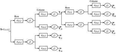
where Y NA denotes the approximation at level N and Y NH(V/D) the horizontal (vertical/diagonal) detail coefficients; ↓2 denotes that the size of the matrices have been downsized by a factor of 2 at each step (adapted with permission from N. Kingsbury [2003] from original material published online at http://http://cnx.rice.edu/content/m11140/latest/). Hence, the filters effectively perform the subspace projections (low pass onto scaling subspaces and high pass onto wavelet subspaces).
APPENDIX B.
DEFINITIONS OF SPATIAL AND TEMPORAL (CROSS‐) CORRELATIONS AND SPECTRA
Both correlation and spectral functions express the statistical covariation within and between signals, although in slightly different ways (the spectra provide a frequency decomposition of the correlation functions). In this appendix, we first provide a qualitative description of the correlation and cross‐correlation functions and then mathematical derivations of spatial and temporal spectra and cross‐spectra. The mathematical definitions are given in spectral form since these are plotted in the figures of this study. A brief discussion of the concept of “stationarity” is also given.
Qualitative Description
In a spatiotemporal data set, such as fMRI, there are temporal correlations within a single pixel's time series and spatial correlations within a given slice at a particular time. There also exist temporal cross‐correlations between two pixels' time series and spatial cross‐correlations between two slices (or between the same slice recorded at different times). More specifically, suppose we have two time series, y 1(t) and y 2(t). Then the temporal correlation function Γ(y 1;τ) expresses the average co‐variation of all pairs of elements {y 1(t), y 1(t+τ)} separated by a time lag of τ within y 1. The temporal cross‐correlation function ΓC(y 1,y 2;τ) expresses the average co‐variation of pairs taken one from each time series {y 1(t),y 2(t+τ)}, again separated by a time lag τ.
If we have two images, S 1(x) and S 2(x) then the spatial correlation function Π(S 1;d) expresses the average co‐variation of all pairs of elements {S 1 (x 1), S 1 (x 2)} separated by the Euclidean distance d = |x 1–x 2| taken from S 1. The spatial cross‐correlation function Πc(S 1,S 2;d) expresses the average co‐variation of pairs taken one from each image {S 1 (x 1), S 2 (x 2)}, again separated by d = |x 1–x 2|.
Functional neuroimaging data consists of a series of slices S i(x,t) recorded over a time window t = {t 1,t 2,…,t N}, which in this report are treated as a multivariate two‐dimensional time series. It is thus possible to restrict ourselves to linear subsets (constant space or constant time) of the entire data set and derive the temporal or spatial (cross‐) correlation functions as discussed above. These are examples of specific correlation functions because they have a specific localization in time or space (temporal correlation functions derive from a particular pixel; spatial correlations derive from a slice recorded at a particular time). It is alternatively possible, using the appropriate formula, to calculate a single higher‐order spatio‐temporal correlation function from the entire data set. Subsequent reduction of the dimensionality of such a function can be achieved by integrating over one of more (spatial or temporal) dimensions. For example, integrating over both spatial dimensions yields the temporal correlation function, not of one pixel, but rather an entire slice. Conversely, integrating over the temporal dimension yields the spatial spectra for a slice throughout its temporal recording. This is approximately equal (depending upon the method of integration employed) to the mean temporal correlation function averaged over all pixels. The higher‐order correlation functions represent the correlation structure of the data set and are typical of the data.
Mathematical Formalism
Let S 1 (x,t) and S 2 (x,t) represent the time series recordings of two functional neuroimaging slices where xϵR 2 denotes the position in the plane and t = t 1,t 2,…,t N represents the temporal sequence of recordings. If we choose a spatial position in each slice, x ij = {x i,x j}, then we have two time series, y 1(t) = S 1 (x ij,t) and y 2(t) = S 2 (x kl,t). The discrete Fourier transform operator F yields,
| (A1) |
A(f) and ϕ(f) are the amplitude and phase, respectively, at frequency f=f 1,f 2,…,f N/2 and Δt=t i−t i−1 is the sampling period. The temporal spectral density function (PSD) is simply the square of the amplitude, the modulus squared of the Fourier transform,
| (A2) |
This can also be obtained through multiplication of the Fourier transform with its complex conjugate,
| (A3) |
The temporal cross‐spectral function is, by analogy, defined as the modulus of the cross‐product of the Fourier transform of two time series,
| (A4) |
Note that because this cross‐product is, in general, a complex function, it is necessary to take the modulus to obtain a real‐valued function of frequency f.
If we choose a particular time t = t i, then we have two slices S 1(x) and S 2(x). Because these are two‐dimensional functions, their Fourier transforms are also two‐dimensional (and complex‐valued),
| (A5) |
where f x = {f H,f V} is the two‐dimensional spatial frequency vector. The horizontal spatial spectrum is derived by taking the modulus squared and then integrating in the vertical dimension,
| (A6) |
where the integral is taken over all vertical frequencies f v. The vertical spectrum PSD v is obtained by integrating over f H. As with the temporal spectrum, the spatial cross‐spectra are derived from integrating the modulus of the cross‐products,
| (A7) |
The vertical cross spectrum is likewise derived from integration in the horizontal frequency domain.
As discussed above, it is also possible to calculate higher‐order spatio‐temporal spectra/correlation functions of the entire data set and then integrate over one of more spatial/temporal dimensions. Hence, the temporal spectrum is obtained by integrating the cross‐product over the spatial dimensions
| (A8) |
where f t is the temporal frequency, f = {f t,f x} and F f(S(x,t)) is the three‐dimensional Fourier transform of S. In addition, the horizontal or vertical spatial spectra can be obtained by their appropriate integration,
| (A9) |
These formulae give rise to the plots show in Figures 12 and 13. The spatial and temporal cross‐spectra can be derived by integration of appropriate cross‐products.
Stationarity
The use of temporal and spatial integrals warrants a short discussion about “stationarity.” Obtaining integrals/averages over space or time effectively assumes that the underlying process is stationary in the relevant domain; that is, that the statistical properties are time/space invariant. More specifically, stationarity assumes that, given sufficient length of data, all statistical measures (mean, variance, correlation functions, spectra, kurtosis, etc.) will converge. Finite lengths of data, or subdivisions of the data, yield representative values of such measures, which do not drift in time. This is the usual meaning of the term “stationary” or “ergodic” [see Stam et al., 2003].
The method described in this study rests on the assumption that the physiological data are stationary in both the temporal domain and in the (intra‐cerebral) spatial domain. However, by constraining the randomization procedure, a variety of more complex hypotheses could be tested. By constraining the randomization to within any subdomain of the data does allow non‐stationarity to be accommodated. In fact, this is the very basis of allowing for the irregular intracerebral domain.
REFERENCES
- Andrzejak RG, Kraskov A, Stogbauer H, Mormann F, Kreuz T (2004): Bivariate surrogate techniques: necessity, strengths and caveats. Phys Rev E 68: 066202. [DOI] [PubMed] [Google Scholar]
- Brammer MJ, Bullmore ET, Simmons A, Williams SCR, Grasby PM, Howard RJ, Woodruff PWR, Rabe‐Hesketh S (1997): Generic brain activation in functional magnetic resonance imaging: A non‐parametric approach. Magnet Reson Imag 15: 763–770. [DOI] [PubMed] [Google Scholar]
- Breakspear M, Terry J (2002a): Detection and description of nonlinear interdependence in normal multichannel human EEG. Clin Neurophysiol 113: 735–753. [DOI] [PubMed] [Google Scholar]
- Breakspear M, Terry J (2002b): Topographic organisation of nonlinear interdependence in multichannel human EEG. Neuroimage 16: 822–825. [DOI] [PubMed] [Google Scholar]
- Breakspear M, Brammer MJ, Robinson PA (2003): Construction of multivariate surrogate sets from nonlinear data using the wavelet transform. Physica D 182: 1–22. [Google Scholar]
- Bullmore ET, Brammer MJ, Rabe‐Hesketh S, Curtis VA, Morris RG, Williams SCR., Sharma T, McGuire PK (1999): Methods for diagnosis and treatment of stimulus correlated motion in generic brain activation studies using fMRI. Hum Brain Mapp 7: 38–48. [DOI] [PMC free article] [PubMed] [Google Scholar]
- Bullmore ET, Long C, Suckling J, Fadili J, Calvert G, Zelaya F, Carpenter T, Brammer MJ (2001): Colored noise and computational inference in neurophysiological time series analysis: Resampling methods in time and wavelet domains. Hum Brain Mapp 12: 61–78. [DOI] [PMC free article] [PubMed] [Google Scholar]
- Bullmore ET, Fadili J, Breakspear M, Salvador R, Suckling J, Brammer MJ (2003): Wavelets and statistical analysis of functional magnetic resonance images of the human brain. Stat Methods Med Res 12: 375–399. [DOI] [PubMed] [Google Scholar]
- Daubechies I (1992): Ten lectures on wavelets. Philadelphia: SIAM. [Google Scholar]
- Dolan KT, Spano ML (2001): Surrogate for nonlinear time series analysis. Phys Rev E 64: 046128. [DOI] [PubMed] [Google Scholar]
- Friston KJ, Frith CD, Liddle PF, Frackowiak RSJ (1993): Functional connectivity: the principal component analysis of large (PET) data sets. J Cereb Blood Flow Metab 13: 5–14. [DOI] [PubMed] [Google Scholar]
- Friston KJ, Harrison L, Penny WD (2003): Dynamic causal modeling. NeuroImage 19: 1273–1302. [DOI] [PubMed] [Google Scholar]
- Grecius MD, Krasnow B, Reiss A, Menon V (2003): Functional connectivity in the resting brain: A network analysis of the default mode hypothesis. Pros Natl Acad Sci USA 100: 253–258. [DOI] [PMC free article] [PubMed] [Google Scholar]
- Harrison L, Penny WD, Friston KJ (2003): Multivariate autoregressive modeling of fMRI time series. NeuroImage 19: 1477–1491. [DOI] [PubMed] [Google Scholar]
- Kingsbury N (2003): The 2‐D DWT. The Connections Project. Houston: Rice University. Published online at http://cnx.rice.edu/content/m11140/latest; accession date February 2004.
- Kugiumtzis D (1999): Test your surrogate data before you test for nonlinearity. Phys Rev E 60: 2808–2816. [DOI] [PubMed] [Google Scholar]
- Lahaye PJ, Poline J‐B, Flandin G, Dodel S, Garnero L (2003): Functional connectivity: studying nonlinear, delayed interactions between BOLD signals. NeuroImage 20: 962–974. [DOI] [PubMed] [Google Scholar]
- Laird AR, Rogers BP, Meyerand ME (2004): Comparison of Fourier and wavelet resampling methods. Mag Res Med 51: 418–422. [DOI] [PubMed] [Google Scholar]
- Lowe MJ, Mock BJ, Sorenson JA (1998): Functional connectivity in single and multislice echoplanar imaging using resting state fluctuations. NeuroImage 7: 119–132. [DOI] [PubMed] [Google Scholar]
- Mallat S (1999): A wavelet tour of signal processing. London: Academic Press. [Google Scholar]
- Netoff TI, Schiff SJ (2002): Decreased neuronal synchronization during experimental seizures. J Neurosci 22: 7297–7307. [DOI] [PMC free article] [PubMed] [Google Scholar]
- Peled A (1999): Multiple constraint organization in the brain: a theory for schizophrenia. Brain Res Bull 49: 245–250. [DOI] [PubMed] [Google Scholar]
- Prichard D, Theiler J (1994): Generating surrogate data for time series with several simultaneously measured variables. Phys Rev Lett 73: 951–954. [DOI] [PubMed] [Google Scholar]
- Rapp PE, Cellucci CJ, Watanabe TAA, Albano AM, Schmah TA (2001): Surrogate data pathologies and the false‐positive rejection of the null hypothesis. Int J Bifurcat Chaos 4: 983–997. [Google Scholar]
- Rombouts SARB, Stam CJ, Kuijer JPA, Scheltens Ph, Barkhof F (2003): Identifying confounds to increase specificity during a “no task condition”: Evidence for hippocampal connectivity using fMRI. NeuroImage 20: 1236–1245. [DOI] [PubMed] [Google Scholar]
- Schiff S, So P, Chang T, Burke R, Sauer T (1996): Detecting dynamical interdependence and generalized synchrony through mutual prediction in a neural ensemble. Phys Rev E 54: 6708–6724. [DOI] [PubMed] [Google Scholar]
- Schreiber T (1998): Constrained randomization of time series data. Phys Rev Lett 80: 2105–2108. [Google Scholar]
- Schreiber T, Schmitz A (1996): Improved surrogate data for nonlinearity tests. Phys Rev Lett 77: 635–638. [DOI] [PubMed] [Google Scholar]
- Schreiber T, Schmitz A (2000): Surrogate time series. Physica 142D: 346–382. [Google Scholar]
- Stam K, Breakspear M, vanCappellenvanWalsum AM, van Dijk BW (2003): Nonlinear synchronization in EEG and whole‐head MEG recordings of healthy subjects. Hum Brain Mapp 19: 63–78. [DOI] [PMC free article] [PubMed] [Google Scholar]
- Theiler J, Eubank S, Longtin A, Galdrikian B, Farmer J (1992): Testing for nonlinearity: the method of surrogate data. Physica 58D: 77–94. [Google Scholar]
- Varela F, Lachaux JP, Rodrigeuz E, Martinerie J (2001): The brainweb: Synchronization and large‐scale integration. Nature Neurosci 2: 229–239. [DOI] [PubMed] [Google Scholar]
- Williams LM, Brammer MJ, Skerrett D, Lagopolous J, Rennie C, Kozek K, Olivieri G, Peduto T, Gordon E (2000): The neural correlates of orienting: An integration of fMRI and skin conductance orienting. Neuroreport 11: 3011–3015. [DOI] [PubMed] [Google Scholar]
- Xiong J, Parson LM, Gao JH, Fox PT (1999): Interregional connectivity to primary motor cortex using resting state images. Hum Brain Mapp 8: 151–156. [DOI] [PMC free article] [PubMed] [Google Scholar]
Associated Data
This section collects any data citations, data availability statements, or supplementary materials included in this article.
Supplementary Materials
This article contains supplementary material, in the form of visual animations of original and wave‐strapped surrogate data, which can be found online at http://www.interscience.wiley.com/jpages/1065-9471/suppmat
Supporting Information file suppmat_1957.pdf
Supporting Information file suppmat_1957_movie1.avi
Supporting Information file suppmat_1957_movie2.avi
Supporting Information file suppmat_1957_movie3.avi
Supporting Information file suppmat_1957_movie4.avi