Nonlinear analysis of EEG during NREM sleep reveals changes in functional connectivity due to natural aging

Abstract

The spatial organization of nonlinear interactions between different brain regions during the first NREM sleep stage is investigated. This is achieved via consideration of four bipolar electrode derivations, Fp1F3, Fp2F4, O1P3, O2P4, which are used to compare anterior and posterior interhemispheric interactions and left and right intrahemispheric interactions. Nonlinear interdependence is detected via application of a previously written algorithm, along with appropriately generated surrogate data sets. It is now well understood that the output of neural systems does not scale linearly with inputs received and, thus, the study of nonlinear interactions in EEG is crucial. This approach also offers significant advantages over standard linear techniques, in that the strength, direction, and topography of the interdependencies can all be calculated and considered. Previous research has linked delta activity during the first NREM sleep stage to performance on frontally activating tasks during waking hours. We demonstrate that nonlinear mechanisms are the driving force behind this delta activity. Furthermore, evidence is presented to suggest that the aging brain calls upon the right parietal region to assist the pre‐frontal cortex. This is highlighted by statistically significant differences in the rates of interdependencies between the left pre‐frontal cortex and the right parietal region when comparing younger subjects (<23 years) with older subjects (>60 years). This assistance has been observed in brain‐imaging studies of sleep‐deprived young adults, suggesting that similar mechanisms may play a role in the event of healthy aging. Additionally, the contribution to the delta rhythm via nonlinear mechanisms is observed to be greater in older subjects. Hum. Brain Mapping 23:73–84, 2004. © 2004 Wiley‐Liss, Inc.

INTRODUCTION

Until recently, typical investigations of connectivity between different regions of the brain have generally employed linear measures of interdependence, such as the calculation of the coherence between two channels. Achermann and Borbély [1998] used the coherence function to illustrate strong coherence of sleep spindles across the scalp, and sleep‐stage‐dependent changes in coherence in different brain regions. However, Chang et al. [Chang et al., 2000], when considering rhythm generation in chains of multiple oscillations, showed that population metastability was achieved via a combination of linear and nonlinear dynamical interactions. Furthermore, it was suggested that such stable rhythms in populations of coupled oscillators could be achieved even in the absence of mutual entrainment.

An interest in modelling complex system behaviour such as the signals recorded via EEG requires an understanding of the dynamic process that generated the collected data. Thus motivated, some recent progress has been made in the development of techniques for distinguishing underlying deterministic nonlinear behaviour from stochastic oscillations in time‐series data [Schiff et al., 1996; Terry and Breakspear, 2003]. These studies have used local linear approximations to reconstructed orbits, in order to predict the evolution of errors between the actual orbit and the predicted value. The manner in which these prediction errors grow can be used to statistically determine whether the underlying process was a deterministic nonlinear process or a stochastic linear process. Thus, distinguishing between these types of process is crucial if we are to subsequently model the process in a suitable manner. Several recent reports have subsequently employed these techniques to detect the occurrence of strongly nonlinear interactions between channels in both scalp [le Van Quyen et al., 1999] and intracranial recordings [Arnhold et al., 1999] in the buildup to and during epileptic seizures. In certain types of seizure, of the temporal lobe for example, the seizure activity appears at some focal point and entrains the activity in other brain regions via some nonlinear synchronization type mechanism. It seems that the appearance of consistent bursts of strong nonlinear interdependence between EEG channels, reflects the abnormally strong nonlinear synchronous oscillations of neuronal activity arising in the cortex. As such, nonlinear synchronization in this context can be viewed as somewhat negative. However, synchronous cortical activity in normal cognitive function has been studied on a number of occasions and synchronization has been proposed as a mechanism by which functional integration between specialized neural networks can be achieved [Gray et al., 1989; Haig et al., 2000; Rodriguez et al., 1999]. Friston [1997] suggests that nonlinear mechanisms may play a crucial role in connectivity in large‐scale neural networks, where nonlinear interactions may facilitate integration between distributed neural systems, which each exhibit distinct local activity. Therefore, understanding the interplay between too little and too much synchrony is an important question that needs addressing. One possible answer is that the local nonlinear dynamics of different brain regions are typically in an intermittent state [Platt et al., 1993] where there are short periods of synchronization together with large deviations from the synchronous state(s). These types of behaviour have been investigated numerically in a neurophysiological model [Breakspear et al., 2003b] as well as experimentally, where the presence and patterns of nonlinear interdependence in scalp EEG in normal subjects [Breakspear and Terry, 2002a, b] and in those suffering from schizophrenia [Breakspear et al., 2003c] were investigated.

Furthermore, the study of nonlinear interactions using techniques for detecting nonlinear interdependence, as opposed to investigating purely linear interactions using the coherence function, has the additional benefit that the direction of the interactions can be determined. Using linear coherence, a measure of interdependence between two systems is determined. However, it is not possible to distinguish whether the first system was driving the second system or vice versa. In contrast, the techniques used in this report make it possible to distinguish between the different states of interaction. The ability to determine which brain region is responsible for the synchronicity is crucial for making conclusions about how brain regions integrate together.

In the previous studies utilizing nonlinear interdependence‐based techniques, the focus was on an eyes‐open, eyes‐closed regime. However, in this report we attempt to focus on latent connectivity by studying data collected from subjects during sleep. Specifically, 16 subjects were subdivided into two groups: young subjects (<23 years old) and older subjects (>60 years). This type of study offers a number of advantages over previously collected data, particularly reduction in noise levels due to, for example, electromyogenic artifacts, eye movements, and other distractions. It also provides the opportunity to examine age‐specific differences in brain connectivity and contributions of nonlinear mechanisms to different rhythms.

For example, the delta rhythm has been proposed as an indication of “recovery” for the resting cerebrum [Werth et al., 1996, 1997] and shows large age‐related differences in amplitude and frequency [Wauquler et al., 1989]. Until now only the contribution of linear mechanisms to delta activity has been investigated [Achermann and Borbély, 1998]; however, recent results on nonlinear contributions to the alpha rhythm during wake [Breakspear and Terry, 2002a] suggests that the contribution of nonlinear mechanisms to the delta rhythm should also be investigated further.

Previous work has described how delta activity in the frontal region during the first NREM period is linked to performance on frontally activating tasks during wakefulness [Anderson and Horne, 2003], suggesting that the general ability of the Pre‐Frontal Cortex (PFC) is reflected in both neuropsychological performance and “recovery” sleep at night. Hence, any significant findings during the first NREM period may reflect daytime executive function.

Interesting developments indicate that the PFC, notably the left PFC, seems vulnerable to sleep deprivation [Horne, 1993; Thomas et al., 1998] and natural ageing [Harrison et al., 2000; West, 1996]. Furthermore, brain imaging during sleep deprivation has indicated that the PFC recruits other brain regions (particularly the right parietal) as a compensatory measure to assist the PFC [Drummond et al., 2000, 2001]. Whether this type of mechanism has a similar compensatory effect, as the brain naturally ages, is currently unknown. Therefore, it is of particular interest to examine whether there are significant differences in the topography of interdependencies between the two age groups, as this may highlight possible deterioration of the PFC, due to natural aging.

In order to consider these connections, four bipolar electrode derivations, Fp1F3, Fp2F4, O1P3, O2P4, were chosen to represent frontal and posterior and interhemispheric interactions, and left and right‐sided intrahemispheric interactions. We analysed this collected data using software developed in Matlab (Mathworks, Natick, MA) based upon the nonlinear interdependence detection algorithm introduced in Terry and Breakspear [2003]. A detailed description of this algorithm is presented in the following section.

The rest of this report is organized as follows. The following section is concerned with the selection of subjects and on how the overnight EEG data were obtained. Subsequently, we describe the statistical methods used to analyse the collected data, focusing in particular on the construction of appropriate surrogate data sets. We then present the results and a discussion of our analysis.

SUBJECTS AND METHODS

In this section, we discuss the procedure for selecting the subjects studied in this report and describe the techniques used to acquiring the data and for the statistical analysis carried out.

Participants

Sixteen healthy adults (8 men, 8 women) were recruited via advertisement and subdivided into two groups: young (range 19–22 years; mean age: 21.02 ± 1.05 years) and older (range 61–75 years; mean age: 65.8 ± 2.8 years). The subjects were screened to exclude those with anything other than minor ailments, or those who were taking medications other than anti‐inflammatory agents (e.g., those on β‐adrenergic receptor‐blocking agents, antidepressants, and hypnotics). The subjects were right‐hand dominant (determined by the Edinburgh Handedness Inventory) [Oldfield, 1971]. Further, they also underwent a sleep screening procedure to exclude those with possible sleep disorders or sufferers of excessive daytime sleepiness. All subjects subsequently underwent overnight EEG recordings (see Electroencephalogram Recordings), which also acted as a final screening for abnormal sleep disturbance.

The study was approved by the Loughborough University Ethical Committee and participants were paid for their involvement.

Design and Procedure

Sleep EEG recordings and electrode application were undertaken at home for 2 nights, on weekdays, 5 to 7 days apart. Home rather than laboratory recording was utilized because it is typical for participants to prefer having data collected in this manner. In particular, we previously found that older people can become apprehensive about sleeping away from home, in a laboratory setting, and that without extensive adaptation to the laboratory, their sleep is impaired. The first night was used for adaptation purposes and the data collected were not used in the statistical analysis. They retired to bed at their usual times, resulting in all bedtimes being between 23:00h and 00:30h, and all arising times between 06:45h and 08:00h. Participants were required to abstain from consuming caffeinated drinks (including strong tea) and alcohol after 18:00h on the evenings of the sleep recording.

Electroencephalogram Recordings

EEG recordings were made with an ambulatory 8‐channel polygraph (Embla Medical Devices, Reykjavik, Iceland). The EEG montage divided the cortex into quadrants as determined by Fp1–F3, Fp2–F4, O1–P3, O2–P4. To avoid confounding of inter‐electrode coherence due to the effects of the common reference electrode, bipolar derivations were used [Fein et al., 1988]. Nunez et al. [1997] have shown that these exclude activity from a number of remote sources (including the reference electrode) by producing a spatially high‐pass filtered estimate of local activity. Within participants, the 4 bipolar EEG interelectrode distances were the same, and EEG electrode impedances were maintained at less than 5 kOhm. High‐pass digital filtering (using finite impulse response digital filters) was set at 0.3 Hz, which had little effect on activity greater than 0.5 Hz. Low‐pass filtering was set at 40 Hz. The sigma–delta A/D converter used by the Embla EEG recording system has an anti‐aliasing filter in front of the sigma‐delta conversion. It has anti‐aliasing filters before each decimation stage. The last anti‐aliasing filter is set at 45 Hz when sampling at 100 Hz.

Traditionally, the sleep EEG is divided into 30‐ or 60‐sec epochs and divided up into six stages, including interim wakefulness, as well as REM (rapid eye movement) sleep and non‐REM stages 1–4. The latter are of increasing depth and differ primarily in the amount of high amplitude delta (0.5–3.5 Hz) activity they contain. Thus, stage 1, a transient phase between wakefulness and stage 2 sleep, contains no appreciable delta activity, and largely consists of low amplitude theta (4–7 Hz) activity, episodic vertex sharp waves, and spindle (11–15 Hz) bursts of less than 500‐msec duration. Stage 2 is the most abundant stage, and largely comprises longer bursts of spindle activity and isolated delta waves in the form of K complexes. Stage 3 is an interim stage between stages 2 and 4, and contains between 20% and 50 high amplitude delta activity. When the latter exceeds 50%, the epoch becomes stage 4. Stages 3 and 4 combined are collectively known as slow wave sleep (SWS). The EEG of REM sleep is similar to that of stage 1, but without spindles or sharp waves, and is characterised by the eye movement bursts. REM sleep occurs about every 90 min, lasting for about 20–30 min. SWS is most profound shortly after sleep onset and is largely contained in the first non‐REM period, i.e., the time between sleep onset and the first REM episode. Some SWS is found in the second non‐REM period and relatively little thereafter, when most of subsequent non‐REM sleep consists of stage 2. We, therefore, focused on data from the first NREM period as it contains the largest portion of delta activity and is less problematic with regard to intervening wakefulness, compared with subsequent periods.

The NREM episode was deemed to begin 10 min into the first period of uninterrupted (stage 1 and 2) sleep after lights out and to terminate at the beginning of the first indication of a greater than 30‐s period of REM sleep [Rechtschaffen and Kales, 1968]. This 10‐min criterion also excluded most slow eye movements because most participants were well into stage‐2 sleep. At least 95% of each participant's EEG data from the first NREM period was free of artifact (which usually occurred as a result of the electromyogram [EMG]).

Nonlinear Interdependence and the Algorithm Employed for Detection

The underlying assumption in the analysis presented in this report is that the brain may be thought of as a large network of coupled nonlinear dynamical systems. The discussion that follows of how this assumption can be employed to detect synchrony between neural regions is adapted from earlier work of one of the authors [Breakspear and Terry, 2002b]. From the early work of Freeman [1975] through to the present day there have been many studies that support the idea that there is not a single global state for the brain but rather the local dynamics and perhaps more importantly the integrations between these states are the significant factor.

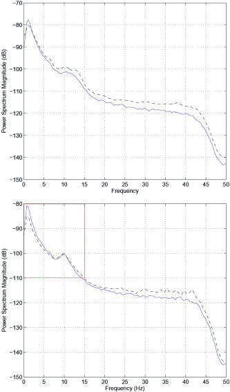
Suppose that there two systems exists evolving in phase spaces X and Y, respectively, and that x(t), y(t) represent the state‐space variables of these systems. The time evolution of these systems may be thought of as the flow generated by:

f and g are nonlinear functions that generate the local dynamics, and these dynamics may be chaotic. The function h introduces the influence of the system X on the system Y. Since there is no reciprocal relationship between Y and X, the system X is referred to as the driver, and the system Y the response or driven system. The strength of this influence is parameterized by the set of coupling parameters c. These parameters are chosen in such a way that h ₀ = 0 and, therefore, in the absence of coupling, the two systems evolve independently in the total phase space X ⊕ Y; As the coupling strength is increased, the dynamics of the two systems X and Y start to interact and in this setting become confined to a smaller region of the total phase space. For coupling of a sufficient strength, the dynamics of the full system collapse onto a lower dimensional manifold called the synchronization manifold [Josic, 1998] and in this scenario the two systems are said to exhibit generalized synchronization [Abarbanel et al., 1996 Rulkov et al., 1995]. This corresponds to

where ϕ is a function, which as a minimum requirement is almost everywhere continuous and one‐to‐one. This relationship implies that it is possible to determine the dynamics of the driven system Y, given orbits of the driver X. It is this relationship that underpins the detection of nonlinear interdependence in the method subsequently described.

Currently, mathematical constraints require that the theoretical discussion of generalized synchronization be limited to the case of drive‐response systems. However, these types of relationships have been commonly observed in mutually coupled systems and in numerical simulations [presented in Terry and Breakspear, 2003], the algorithm used worked well in the case of mutual coupling, weak coupling, system noise, and measurement error.

The issue that remains to be overcome is that the state variables x(t) and y(t) are not directly accessible. Instead we have some measured scalar variables (in this particular situation, those collected from the EEG channels),

where k is some (possibly nonlinear) measurement function and ε_1,2(t) are white noise processes, associated with corruption of the signal by measurement noise. In this setting, the original state‐space variables are recovered from the EEG recordings using time‐delay embedding [Takens, 1981]. These EEG recordings, are a reflection of summed local field potentials generated by cortical networks [Nunez, 1995], with coupling arising primarily as the result of spare long‐range excitatory projections.

This time‐delay embedding technique utilized requires the dimension d in which to embed and the time‐delay τ with which to delay. There are many techniques available to determine embedding dimension and we used the method of false nearest neighbors suggested in Kennel et al. [1992]. The time‐delay was chosen to be the correlation time divided by d − 1 [Albano et al., 1988] (in the data analysed, d = 5, τ = 7). For a pair of bipolar derivations, reconstructed orbits were obtained from the normalized recordings V̂ _i, V̂ _j having the form:

These time‐series correspond to reconstructed orbits in the phase spaces X and Y. To test for nonlinear interdependence between these two time‐series, the algorithm of Terry and Breakspear [2003] was used. The algorithm was applied to the collected data in sequential epochs, each containing 1,024 data points, where the data was sampled at a frequency of 100 Hz. This nonlinear measure of predictability employed offers a number of advantages over linear coherence, such as sensitivity to direction of influence and determination of interdependence between different types of activity. It is also possible to classify the strength of such interactions.

Essentially this algorithm determines the presence of nonlinear interactions between the two systems as follows. At time t = t _i , construct a simplex around x(t _i) consisting of 2d ₁ vertices in the phase space X, where each vertex is another member of the reconstructed orbit x(t). These vertices are chosen in such a way that the volume of the simplex is minimized, whilst maintaining computational efficiency. For certain time points, it may not be possible to condatamaticsch a simplegips the values may lie on the extrema of the orbit. In this situation, the missing vertices are replaced by a sufficient number of nearest neighbors.

Indexing the vertices chosen by their time points t _j , we may then construct a simplex in the phase space Y using the equivalent vectors. By taking a weighted average of these vertices (essentially obtaining the centre of mass of the simplex), we discover an approximation to the vector y(t _i) as predicted by knowledge of the vector x(t _i). We then compare the predicted and actual values of y(t _i) and obtain a prediction error. This error is then normalized by calculating another prediction to y(t _i), only this time by use of a simplex whose vertices are randomly chosen and the average of these is weighted with respect to another randomly chosen point.

In the absence of interdependence, there is no reason to assume that the predicted value as chosen by the optimal simplex for x(t _i) should be any better than that of a randomly chosen simplex, so it should assume an value of ∼1. The presence of interdependence reduces this error, depending on how well the orbits of X predict those of Y. If these are identical, then the error should be approximately 0.

The final step for demonstrating that this relationship is deterministic (as opposed to stochastic) is to attempt to predict future iterates of the orbit in a similar manner. This is achieved by calculating the simplex in Y as above and then iterating H steps along the respective orbits of each vertex. The weighted predicted value is again compared with the actual value and the error calculated and normalized. This leads to H prediction errors; an example of this can be seen in figure 5 of Breakspear and Terry [2002b].

Figure 5.

Correlation coefficients for the concurrent occurrence of nonlinear interdependence in either direction between different bipolar electrode derivations in the case of young subjects. F, frontal; P, parietal; L, left; R, right. The bold arrows represent the reference pairing and the values denote the correlation coefficients for nonlinear interdependence in either direction of the adjacent arrow pairing relative to the reference pair. P values for these coefficients were all less than 0.01.

If the processes were actually generated by uncorrelated white noise, the prediction error should jump to 1, for H = 1. If the two systems are generalized synchronized, then this error should grow at a rate proportional to the largest Lyapunov exponent. If the interdependence is weak, some future predictability is possible, but the error will grow more rapidly than that determined by the largest Lyapunov exponent and will approach 1 in fewer time steps.

This relationship may be determined in the opposite direction by interchanging X and Y and their corresponding vectors.

Unfortunately, the final step has a slight sting in its tail, in that although uncorrelated white noise will give maximums of 1 after just one time‐step, for linearly correlated colored noise, the prediction errors will be less than 1 for some future values H. Hence the prediction errors must be statistically compared to those calculated from appropriately generated surrogate data, where linear correlations are preserved but nonlinear interdependencies (if they exist) are destroyed.

Surrogate data analysis

For each subject, 49 surrogate data sets were constructed from randomly chosen epochs within each subject's data. Since the comparison of surrogate data to individual epochs is a one‐tailed test, 49 sets are required in order to test statistically at the 1% level. It could be argued that one should generate 49 surrogate sets per epoch, rather than comparing each epoch to a static 49 data sets. However, this is for computational reasons unrealistic as it would require analysing at least 3,430 surrogate data sets per subject, as opposed to 49. These surrogate sets were calculated using a phase‐randomized, amplitude‐adjusted algorithm, based upon the work of Theiler et al. [1992], Pritchard and Theiler [1994], and Rombouts et al. [1995]. For each subject, the mean and standard deviation for each prediction error were computed from this overall ensemble, representing the values used to compare each epoch with the null hypothesis in each subject. These are then used to allow accurate calculation of the 99% confidence intervals. P values were then obtained via a one‐tailed parametric test, representing the probability that the experimental measures would be observed by chance alone, given that the null hypothesis of purely linear interactions was correct. The Keppel correction [Keppler, 1991] to control for repeated observations was not employed in this analysis, as it is believed to give an overly conservative indication of nonlinear interactions (Friston, 2002, personal communication).

If an epoch contained at least one nonlinear index outside this corrected interval, then it was identified as exhibiting nonlinear interdependence. The strength of nonlinear interdependence was determined by the number of indexes outside of the confidence interval for each epoch. This calculation was performed in both directions for each combination of bipolar pairs.

Recently, work has appeared regarding the use of wavelet resampling for generating surrogate data sets [Breakspear et al., 2003a]. This type of technique is particularly important, for example, in fMRI where there is essentially spatial continuity. However, in the EEG analysis presented here, space is discrete and the traditional Fourier based techniques utilized are suitable for the surrogate data generation.

Summary

The algorithm may be summarized as follows:

• 1For each epoch, we reconstruct the orbits from each EEG channel using a time‐delay embedding technique [Takens, 1981].
• 2We then choose appropriate local linear maps for each point along the orbit of system one and use these to attempt to predict the future evolution of the orbits of system two.
• 3If this prediction is better than that of a randomly chosen map, then there is potentially nonlinear interdependence between system one and system two.
• 4To confirm this is the case, a comparison is made between that of the epoch and that from appropriately generated surrogate data. This is to control for limitations of the data, such as the presence of linear coherence, colored noise (which has a power‐frequency relationship), a finite sample size, sampling error and measurement noise. All of these are known to permit inaccurate detection of nonlinearity.

A more detailed overview of the methods employed in this report is given in Breakspear and Terry [2002b] and Terry and Breakspear [2003].

Topography of Interdependence

It has been hypothesized that nonlinear coupling between brain regions (and hence nonlinear interdependence between EEG channels) would not occur as an isolated phenomenon, but would occur in different spatial patterns. In order to study the topography of nonlinear interactions between different brain regions, we investigated the relationship between the indices of interdependence. This involved selecting an “index” bipolar pair, Fp₁F₃/Fp₂F₄ for example, then establishing which epochs exhibited nonlinear interdependence between this pair. Subsequently, the correlation coefficients between the indices of the index pair and those of each other pairwise combination were evaluated. The occurrence of nonlinear interdependence can occur in consecutive epochs in each electrode pair, which can cause autocorrelations within the sequences of indices. These autocorrelations can become reflected in the cross‐correlations and consequently generate disproportionately high correlation coefficients between pairs.

To account for these autocorrelations, the confidence intervals for the null hypothesis were calculated from the surrogate data in the following way. For each sequence of nonlinear interdependencies, a number n, was selected randomly, such that 1 ≤ n ≤ N, where N was the total number of epochs considered (N = 587 for the old subjects and 567 for the young subjects). Subsequently, this sequence was then reordered beginning with the n th index and proceeding to the final index, then beginning with the first index, up to the n − 1‐th index. This shuffling has the effect of preserving autocorrelations in each sequence, but removing linear correlations [Breakspear and Terry, 2002b]. The values calculated are then significant at the 99% level, hence values greater than 0.01 can be considered as being a greater probability than that of chance alone.

Unlike with the coherence function, these coefficients will not necessarily be symmetrical. This is because with the nonlinear interdependence algorithm employed, X → Y is not equivalent to X ← Y, whereas with the coherence function it is only possible to determine X ↔ Y. This is a crucial difference between the two methods and one that allows us to build a “map” of the connectivity in the human brain by use of the different EEG channels.

RESULTS AND DISCUSSION

The main questions we wish to address concern the occurrence of nonlinear interactions between brain regions during sleep. From a basic research perspective, are these interactions more or less prevalent than was the case in previously studied wake data [Breakspear and Terry, 2002a, b], or is the occurrence broadly similar in both cases? Furthermore, are there any changes in the topography of interactions present in the data analysed?

Recent brain imaging studies [Drummond et al., 2000, 2001] of sleep‐deprived young adults indicate that specific brain regions, such as the right parietal area, are activated as a compensatory response for localised areas, known to be affected by sleep loss (i.e., the PFC). As recent research has suggested similar effects caused by natural ageing and sleep deprivation, we are interested from a neuropsychological perspective whether there are statistically significant differences both in the power spectra of NREM EEG in both age groups and also in the topography of interdependencies between brain regions. Of special interest will be the topography when the left frontal–right parietal connection is used as a reference, as this could highlight similar effects via EEG to that previously observed in fMRI.

Prevalence of the Epochs Exhibiting Nonlinear Interdependence

For the whole data set analysed, the number of epochs exhibiting nonlinear interdependence in each respective direction is presented in Table I. The total number of epochs that exhibited nonlinear interdependence in either direction varied from 4.4% to 9.6% across all subjects. These figures are higher than those in Breakspear and Terry [2002a, b] for a number of reasons. First, the analysis performed in our previous studies was overly conservative for reasons discussed above. Secondly, levels of noise and artifact are greatly reduced in sleep EEG as opposed to wake EEG and this will have had a potentially noticeable effect on the performance of the nonlinear detection algorithms utilised, since all of these are susceptible to the effects of measurement noise.

Table I.

Epochs permitting rejection of the null hypothesis of purely linear interactions between bipolar channels

Subjects	Bipolar combination	R to L	L to R	B to F	F to B
Old (587 epochs)	Fp1F3/Fp2F4	44 (7.50)	25 (4.26)	—	—
	O1P3/O2P4	42 (7.16)	21 (3.58)	—	—
	Fp1F3/O2P4	39 (6.64)	34 (5.79)	—	—
	O1P3/Fp2F4	27 (4.60)	20 (3.41)	—	—
	Fp1F3/O1P3	—	—	34 (5.79)	20 (3.41)
	Fp2F4/O2P4	—	—	24 (4.09)	23 (3.92)
Young (567 epochs)	Fp1F3/Fp2F4	25 (4.41)	39 (6.88)	—	—
	O1P3/O2P4	35 (6.17)	34 (6.00)	—	—
	Fp1F3/O2P4	36 (6.35)	24 (4.23)	—	—
	O1P3/Fp2F4	36 (6.35)	32 (5.64)	—	—
	Fp1F3/O1P3	—	—	42 (7.41)	29 (5.11)
	Fp2F4/O2P4	—	—	37 (6.53)	32 (5.64)

Values are expressed as n (%).

In keeping with previous studies, there were no significant differences between frontal and posterior occurrences of nonlinear interdependencies. The number of left‐right interactions was also comparable across all subjects. This should not be construed as a negative finding, since it is often the connectivity between brain regions that is of particular interest, rather than simply the occurrences of interactions between any specific brain regions.

For each of the 16 subjects (8 young, 8 old), we analysed between 70 and 80 1,024‐point epochs. These totalled 567 epochs in the case of the young subjects and 587 epochs for the old subjects. This gave a total of 13,848 pairwise combinations of bipolar derivations investigated.

Power Spectrum Analysis

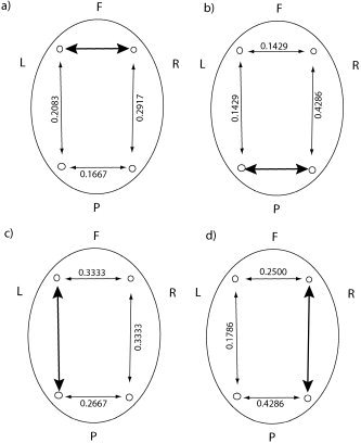
A typical power spectrum from the EEG collected during this stage of sleep is characterized by a peak in power between 1 and 3 Hz. Oscillations with frequency in this region are known as delta (δ) rhythms. In addition, there is another peak at approximately 10 Hz. This secondary peak could be an α – δ resonance due to frontal α activity or it could be a variant of sleep‐spindles. An illustrative example of such a power spectrum is presented in Figure 1.

Figure 1.

Illustrative example of the power‐spectrum from an older subject during NREM sleep. The channel under consideration is FP₁–F₃. The peak in δ‐power at approximately 1.5 Hz and a peak corresponding to sleep‐spindles are also visible. An interesting question is whether linear or nonlinear mechanisms are primarily responsible for the generation of these oscillations.

An important question to address is the relative contributions to these oscillations made by linear and nonlinear mechanisms. In order to achieve this, we subdivided the time‐series of each subject into epochs where the null hypothesis of purely linear interactions between regions could be rejected (i.e., where nonlinear interdependence was detected) and those for which the null hypothesis could not be rejected. We then plotted the power spectra for each case and compared the magnitude of the peaks for each subject (Figs. 2 and 3). Interestingly, the peak in δ power was much more pronounced in those epochs exhibiting nonlinear interdependence relative to those epochs for which the null hypothesis could not be rejected. However, in the case of the 10‐Hz peak, there was no such noticeable difference in the peaks between linear and nonlinear oscillations.

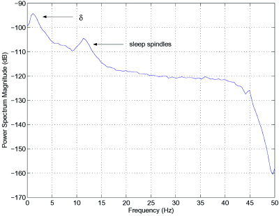
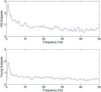
Figure 2.

Spectral properties of all epochs identified as containing nonlinear interdependence (blue/solid) in comparison to all other epochs, for which the null hypothesis could not be rejected (black/dashed). Top: Results of the young subjects. Bottom: Results of the old subjects. Interestingly, the peak in δ‐power is much more pronounced in those epochs exhibiting nonlinear interdependence, as opposed to those for which the null hypothesis could not be rejected. Contrastingly, the peak in power at 12 Hz shows no such difference in the ration of power in nonlinear vs. linear epochs. This is an important point, since it indicates that nonlinear mechanisms are not necessarily the driving force behind all rhythms in the brain. The boxed portion of the spectrum (bottom) is illustrated in Figure 3. This figure was produced using a moving Hanning window of 256 samples.

Figure 3.

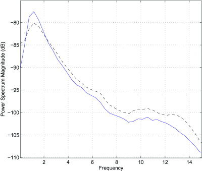
Close‐up of the power spectrum density in the case of old subjects. The difference in δ‐power between nonlinear epochs (blue/solid line) and all others (black/dashed line) is clearly visible. In addition, the closeness between the two in sleep spindles power is also noticed. This suggests that nonlinear mechanisms are responsible for generation of δ waves, but that nonlinear mechanisms do not generate sleep spindles.

To illustrate this difference more clearly, we took Fp ₁ F ₃‐O ₂ P ₄ as the reference pairing for both the younger and older subject groups. We then plotted the average ratio in power spectra between those epochs exhibiting nonlinear interdependence between these two electrodes and those for which the null hypothesis was not rejected (Fig. 4). In both young and old subjects, a maximum in this ratio occurs at the δ‐frequency, whereas no equivalent maximum occurs in the 10‐Hz range. It is also apparent that this ratio between nonlinear epochs and all others is noticeably greater in the old subjects than the young subjects. This is an interesting development, the cause for which cannot be conclusively given but can be speculated upon. From an information‐processing viewpoint, much greater quantities of information can be transmitted via nonlinear mechanisms, due to utilisation of multiple frequencies simultaneously. Hence, one explanation for this increase in the ratio between nonlinear epochs and all others in the case of older subjects, is that the left pre‐frontal cortex is having to call upon the right parietal region in order to maintain the equivalent performance of the younger human brain. We should emphasize at this point that this deterioration can be attributed purely to the effects of natural aging, rather than any known neurological defects in the older subjects.

Figure 4.

Comparison of the ratio of the power spectra between those epochs exhibiting nonlinear interdependence and all others, in the case of old subjects and young subjects. The peak in this ratio in δ‐power indicates that nonlinear mechanisms are the driving force behind these oscillations. Note that there is no equivalent peak in the sleep‐spindles range (9–14 Hz). It is also interesting to observe that the peak in this ratio is noticeably higher for the old subjects.

These observations compare favourably with a previous study of eyes‐open, eyes‐closed data [Breakspear and Terry, 2002a], where the peak in alpha (α) power (10‐Hz oscillations) was significantly more pronounced in those epochs exhibiting nonlinear interdependence, relative to those for which the null hypothesis could not be rejected. This continues to support the theory that nonlinear interactions between brain regions, whilst detected relatively infrequently, are actually the driving force behind many of the common rhythms in the human brain, often making vital contributions.

Correlations Between Nonlinear Interdependencies in Different Bipolar Pairs

We illustrate some of the results for the correlations of nonlinear interdependence between the various combinations of electrode pairs in Figures 5 and 6. In each figure, a “reference” pair is represented by a bold arrow and correlations are then calculated between this pair and all others (light arrows). These correlation coefficients were empirically calculated from the shuffled sequences as described in Topography of Interdependence and had mean 1.1 × 10⁻⁴ and variance 4.9 × 10⁻⁴ for the older subjects and mean 6.7 × 10⁻⁵ and variance 7.8 × 10⁻⁴ for the younger subjects.

Figure 6.

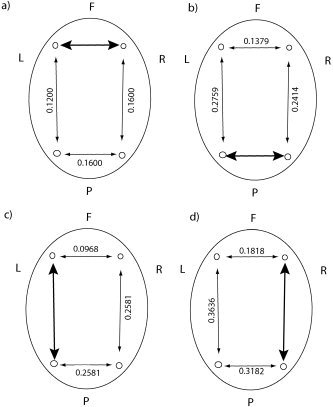
As per Figure 5, but for the old subject group. Again, P values for these coefficients were all less than 0.01.

Bidirectional Correlations for Occurrence of Nonlinear Interdependence Between Bipolar Channels

In both age groups, the correlation coefficients for the occurrence of nonlinear interdependence in either direction between bipolar channels are all highly significant. Were these patterns of interdependence due to chance alone, we would expect to see correlation coefficients of less than 0.01, whereas the actual coefficients are all significantly larger than this value. On the other hand, these correlations do not show any significant differences either between intrahemispheric and interhemispheric interactions within age groups, or even in equivalent interactions between age groups. This is in keeping with previous studies of this type, where the statistical differences in the topography of interactions is more often highlighted when considering directional differences between subject groups.

Furthermore, the equivalent diagrams for correlation coefficients of the diagonal pairings and all others also did not show any subject‐specific differences in the correlation of interdependency.

Correlations in Directional Nonlinear Interdependence Between Bipolar Pairs

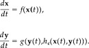
Consideration of direction between all bipolar channels, including diagonally frontal to posterior, reveals far more topographic structure. Of particular interest to us are the coefficients when using the left frontal‐right parietal interaction as a reference. In this situation, illustrated in Figure 7a,b, there are statistically significant differences in these coefficients between the young and old age groups. Of perhaps greater interest is the back connection from right parietal to left frontal, where the correlation coefficient for the old group is 0.5238, relative to 0.2270 for the young group. This suggests that the right parietal regions “talks back” to the left frontal region much more frequently than is the case for the young subjects. This finding is in keeping with the hypothesis that the right parietal region is called upon to assist in normal neural processing as a result of natural aging, and that these changes in plasticity of the connections are highlighted in this topographic analysis. Further evidence of these changes are the significant differences in frontal and parietal interhemispheric interactions between subject groups. The differences in these coefficients are significantly different in the left frontal to right frontal and right parietal to left parietal interactions, providing further evidence of a change in wiring between young and old subjects.

Figure 7.

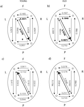
Correlation coefficients for the concurrent occurrence of nonlinear interdependence in either direction between different bipolar electrode derivations. The large bold arrows denote the reference bipolar pair and the direction of interaction. The numbers adjacent to all other arrows are the correlation coefficients for the occurrence of nonlinear interdependence between the bipolar pair in the corresponding direction. a,b: The reference pairing is left frontal–right parietal and statistically significant (bold valued) differences are observed between young and old subjects. Contrastingly, when the reference pairing is right parietal–left frontal (as in c,d) no such statistical differences are observed.

In contrast, when we take the right parietal to left frontal combination as the reference pairing (Fig. 7c,d), no such statistical differences are observed between young and old subjects. This is indicative of the left frontal region being the driving force behind these interactions and that the wirings involved are in the direction left frontal to right parietal only.

It is difficult to make a direct comparison to the previously studied eyes open, eyes closed data [Breakspear and Terry, 2002a, b] since these diagonal interactions were not specifically considered. However, analysis of equivalent pairings to those previously studied did not yield any significant differences in correlations either between subjects in this study or between this study and the previously considered data. For this reason, it was not felt necessary to illustrate these connections.

CONCLUSIONS

In this report, EEG data collected during sleep from 8 older subjects (> 60 years) and 8 young subjects (< 23 years) was investigated using algorithms for the detection of dynamic nonlinear interdependence. The algorithm employed was based upon the theory of coupled nonlinear oscillators, which has recently been widely used for the study of neural function [Breakspear, 2001; Frank et al., 2000]. Specifically, EEG data from NREM sleep stages were investigated, and in this data oscillations at around 1–2 Hz (delta rhythm) and a further peak at 10 Hz were observed to be the dominant frequencies. Interestingly, nonlinear mechanisms were observed to be dominant in the δ region, whereas there was no such dominance in the 10‐Hz range. This finding is both in keeping and in contrast with previous studies of nonlinear interdependence in human EEG [Breakspear and Terry, 2002a, b] where nonlinear mechanisms were observed to contribute strongly to the alpha rhythm.

Perhaps an even more significant observation was the difference in the ratio peaks in power between nonlinear epochs and all others. This ratio peaked in δ‐power and was considerably greater in the old subjects, indicating an increased activity level in neural activity in the left pre‐frontal cortex in the elderly subjects. The precise explanation for this cannot be elucidated and is still under investigation. However, it might, for example, highlight differences in the wiring of the older brain corresponding to a failing of the capabilities of the left pre‐frontal cortex and a need to call upon other brain regions, such as those in the right parietal area, so as to assist in normal brain function.

With regard to connectivity, due to the nature of human EEG, nonstationarity [Palus, 1996] is a potential issue. However, both in our previous study [Breakspear and Terry, 2002b] and in this study, repeated analysis of the data produced remarkably similar results (correlations 0.95). In the present study, the overall occurrences of dynamic nonlinear interdependence were increased on previous studies in wake data. This increase can be attributed in part to a decrease in noise in the system, but also to less conservative corrections of the original statistics. Despite the relatively small number of subjects, statistically significant differences in the topography of interdependencies were also present between young and older subjects and these were particularly apparent when taking left frontal, right parietal interactions as a reference and comparing correlations between this and all other connections. This particular combination was chosen as Drummond and co‐workers [Drummond et al., 1999, 2001] have indicated this connection to be particularly important during working memory tasks, when the PFC is functioning at a less than optimal rate, for example due to sleep deprivation.

It is apparent that the study of nonlinear interdependence in human EEG provides a powerful tool for examining functional connectivity (brain mapping), both in the analysis of sleep EEG data and also for studying performance due to natural aging. The high temporal resolution of EEG makes techniques such as those utilised in this report highly effective and it is also a highly cost‐effective way of obtaining human neural data.

REFERENCES

- Abarbanel HDI, Rulkov NF, Sushchik MM (1996): Generalized synchronization of chaos: the auxiliary system approach. Phys Rev E 53: 4528–4535. [DOI] [PubMed] [Google Scholar]
- Achermann P, Borbély P (1998): Coherence analysis of the human sleep electroencephalogram. Neuroscience 85: 1195–1208. [DOI] [PubMed] [Google Scholar]
- Albano A, Muench J, Schwartz C, Mees A, Rapp P (1988): Singular value decomposition and the grassberger‐procaccia algorithm. Phys Rev A 38: 3017–3026. [DOI] [PubMed] [Google Scholar]
- Anderson C, Horne JA (2003): Pre‐frontal cortex: links between low frequency delta EEG in sleep and neuropsychological performance in healthy, older people. Psychophysiology 40: 349–357. [DOI] [PubMed] [Google Scholar]
- Arnhold J, Grassberger P, Lehnertz K, Elger C (1999): A robust method for detecting interdependencies: application to intracranially recorded EEG. Physica D 134: 419–430. [Google Scholar]
- Breakspear M (2001): A nonlinear model of odor perception by the olfactory bulb. Int J Neural Systems 11: 101–124. [DOI] [PubMed] [Google Scholar]
- Breakspear M, Terry JR (2002a): Detection and description of nonlinear interdependence in normal multichannel human EEG data. Clin Neurophys 113: 735–753. [DOI] [PubMed] [Google Scholar]
- Breakspear M, Terry JR (2002b): Topographic organization of nonlinear interdependence in multichannel human EEG. Neuroimage 16: 822–835. [DOI] [PubMed] [Google Scholar]
- Breakspear M, Brammer MJ, Robinson PA (2003a): Construction of multivariate surrogate data for nonlinear data using the wavelet transform. Physica D 182. [Google Scholar]
- Breakspear M, Terry JR, Friston KJ (2003b): Modulation of excitatory synaptic coupling facilitates synchronization and complex dynamics in a biophysical model of neuronal dynamics. Network Comput Neural Syst 14: 702–732. [PubMed] [Google Scholar]
- Breakspear M, Terry JR, Friston KJ, Harris AJW, Williams LM, Brown K, Brennan J, Gordon E (2003c): A disturbance of nonlinear interdependence in scalp EEG of subjects with first episode schizophrenia. Neuroimage 20: 466–478. [DOI] [PubMed] [Google Scholar]
- Chang HS, Staras K, Gilbey MP (2000): Multiple oscillators provide metastability in rhythm generation. J Neurosci 20: 5135–5143. [DOI] [PMC free article] [PubMed] [Google Scholar]
- Drummond SPA, Brown GG, Stricker JL, Buxton RB, Wong EC, Gillin JC (1999): Sleep dperivation‐induced reduction in cortical functional response to serial subtraction. Neuroreport 10: 1–4. [DOI] [PubMed] [Google Scholar]
- Drummond SPA, Brown GG, Gillin JC, Wong EC, Buxton RB (2000): Altered brain response to verbal learning following sleep deprivation. Nature 403: 655– 657. [DOI] [PubMed] [Google Scholar]
- Drummond SPA, Gillin JC, Brown GG (2001): Increased cerebral response during a divided attention task following sleep deprivation. J Sleep Res 10: 85–92. [DOI] [PubMed] [Google Scholar]
- Fein G, Raz J, Brown F, Merrin E (1988): Common reference coherence data are confounded by power and phase effects. Clin Neurophys 69: 381–384. [DOI] [PubMed] [Google Scholar]
- Frank T, Daffertshofer A, Peper C, Neek P, Haken H (2000): Towards a comprehensive theory of brain activity: coupled oscillators under external forces. Physica D 144: 62–86. [Google Scholar]
- Freeman WJ (1975): Mass action in the nervous system. New York: Academic Press. [Google Scholar]
- Friston KJ (1997): Another neural code? Neuroimage 5: 213–220. [DOI] [PubMed] [Google Scholar]
- Gray C, Konig P, Engel A, Singer W (1989): Oscillatory responses in cat visual cortex exhibit inter‐columnar synchronization which reflects global stimulus properties. Science 338: 334–337. [DOI] [PubMed] [Google Scholar]
- Haig AR, Gordon E, Wright JJ, Maeres RA, Bahramali H (2000): Synchronous cortical gamma‐band activity in task relevant cognition. Neuroreport 11: 1–7. [DOI] [PubMed] [Google Scholar]
- Harrison Y, Horne JA, Rothwell A (2000): Prefrontal neuropsychological effects of sleep deprivation in young adults: a model for healthy aging? Sleep 23: 1067–1073. [PubMed] [Google Scholar]
- Horne JA (1993): Human sleep, sleep loss and behaviour: implications for the prefrontal cortex and psychiatric disorder. Br J Psychiatry 162: 413–419. [DOI] [PubMed] [Google Scholar]
- Josic K (1998): Invariant manifolds and synchronization of coupled dynamical systems. Phys Rev Lett 80: 3053–3056. [Google Scholar]
- Kennel M, Brown R, Abarbanel HDI (1992): Determining embedding dimension for phase space reconstruction using a geometrical reconstruction. Phys Rev A 45: 3403–3411. [DOI] [PubMed] [Google Scholar]
- Keppler G (1991): Design and analysis: a researcher's handbook. New York: Prentice‐Hall. [Google Scholar]
- Ie Van Quyen M, Martinerie J, Adam C, Varela F (1999): Nonlinear analyses of interictal EEG map the interdependencies in human focal epilepsy. Physica D 127: 250– 266. [Google Scholar]
- Nunez P (1995): Neocortical dynamics and human brain rhythms. New York: Oxford University Press. [Google Scholar]
- Nunez P, Srinivassan R, Westdorp A, Wijesinghe R, Tucker D, Silberstein R, Cadusch P (1997): EEG coherency I: Statistics, reference electrode, volume conduction, Laplacians, cortical imaging, and interpretation at multiple scales. Clin Neurophys 103: 499–515. [DOI] [PubMed] [Google Scholar]
- Oldfield RC (1971): The assessment and analysis of handedness: the Edinburgh inventory. Neuropsychologica 9: 97–113. [DOI] [PubMed] [Google Scholar]
- Palus M (1996): Nonlinearity in normal human EEG: cycles, temporal asymmetry, non‐stationarity and randomness, not chaos. Biol Cybernet 75: 389–396. [DOI] [PubMed] [Google Scholar]
- Platt N, Spiegel EA, Tresser C (1993): On‐off intermittency: a mechanism for bursting. Phys Rev Lett 70: 279–282. [DOI] [PubMed] [Google Scholar]
- Pritchard W, Theiler J (1994): Generating surrogate data for time‐series with several simultaneously measured variables. Phys Rev Lett 73: 951–954. [DOI] [PubMed] [Google Scholar]
- Rechtschaffen A, Kales A (1968): A manual of standardized terminology, techniques, and scoring system for sleep stages of human subjects. Los Angeles: Brain Information Service/Brain Research Institute, UCLA. [Google Scholar]
- Rodriguez E, George N, Lachaux N, Martinerie J, Renault B, Varela F (1999): Perception's shadow: long‐distance synchronization of human brain activity. Nature 397: 430–433. [DOI] [PubMed] [Google Scholar]
- Rombouts S, Kuenen R, Stam CJ (1995): Investigation of nonlinear structure in multichannel EEG. Phys Lett A 202: 352–358. [Google Scholar]
- Rulkov NF, Sushchik MM, Tsimring LS, Abarbanel HDI (1995): Generalized synchronization of chaos in unidirectionally coupled chaotic systems. Phys Rev E 51: 980–994. [DOI] [PubMed] [Google Scholar]
- Schiff SJ, So P, Chang T, Burke RE, Sauer T (1996): Detecting dynamical interdependence and generalized synchrony through mutual predection in a neural ensemble. Phys Rev E 54: 6708–6724. [DOI] [PubMed] [Google Scholar]
- Takens F (1981): Detecting strange attractors in turbulence. Lecture Notes Math 898: 366–381. [Google Scholar]
- Terry JR, Breakspear M (2003): An improved algorithm for the detection of dynamical interdependence in multivariate time‐series. Biol Cybernet 88: 129–136. [DOI] [PubMed] [Google Scholar]
- Theiler J, Eubank S, Longtin A, Galdrikian B, Farmer J (1992): Testing for nonlinearity: the method of surrogate data. Physica D 58: 77–94. [Google Scholar]
- Thomas M, Balkin T, Sing H, Wesensten N, Belenky G (1998): PET imaging studies of sleep deprivation and sleep: implications for behaviour and sleep function. J Sleep Res 7: 274. [Google Scholar]
- Wauquler A, Dugovic C, Radulovacki M, editors (1989): Effects of maturation and ageing on slow wave sleep in man: implications for neurobiology in slow wave sleep. Physiological, pathophysiological and functional aspects. New York: Raven Press. [Google Scholar]
- Werth E, Achermann P, Borbély AA (1996): Brain topography of the human sleep EEG: anterior‐posterior shifts of spectral power. Neuroreport 8: 123–127. [DOI] [PubMed] [Google Scholar]
- Werth E, Achermann P, Borbély AA (1997): Fronto‐ocipital EEG power gradients in human sleep. J Sleep Res 6: 102–112. [DOI] [PubMed] [Google Scholar]
- West RL (1996): An application to prefrontal cortex function theory to cognitive aging. Psychol Bull 120: 272–292. [DOI] [PubMed] [Google Scholar]