A method for making group inferences from functional MRI data using independent component analysis

Abstract

Independent component analysis (ICA) is a promising analysis method that is being increasingly applied to fMRI data. A principal advantage of this approach is its applicability to cognitive paradigms for which detailed models of brain activity are not available. Independent component analysis has been successfully utilized to analyze single‐subject fMRI data sets, and an extension of this work would be to provide for group inferences. However, unlike univariate methods (e.g., regression analysis, Kolmogorov–Smirnov statistics), ICA does not naturally generalize to a method suitable for drawing inferences about groups of subjects. We introduce a novel approach for drawing group inferences using ICA of fMRI data, and present its application to a simple visual paradigm that alternately stimulates the left or right visual field. Our group ICA analysis revealed task‐related components in left and right visual cortex, a transiently task‐related component in bilateral occipital/parietal cortex, and a non‐task‐related component in bilateral visual association cortex. We address issues involved in the use of ICA as an fMRI analysis method such as: (1) How many components should be calculated? (2) How are these components to be combined across subjects? (3) How should the final results be thresholded and/or presented? We show that the methodology we present provides answers to these questions and lay out a process for making group inferences from fMRI data using independent component analysis. Hum. Brain Mapping 14:140–151, 2001. © 2001 Wiley‐Liss, Inc.

INTRODUCTION

Independent component analysis (ICA) is a promising data analysis method that is being increasingly applied to fMRI data [Bell and Sejnowski, 1995; McKeown et al., 1998b]. Independent component analysis attempts to separate independent “sources” that have been mixed together (e.g., separating the voices from different speakers recorded on a single microphone). Independent component analysis as applied to fMRI data can be used to separate either spatially [McKeown et al., 1998a] or temporally [Biswal and Ulmer, 1999] independent sources and works well in both situations when appropriate assumptions are met [Calhoun et al., 2001b; McKeown and Sejnowski, 1998].

However, there has not yet been an approach presented for performing an ICA analysis on a group of subjects. This process is complicated by the different processing stages involved in the ICA analysis as well as the computational burden involved. For example, when using the general linear model, the investigator specifies the regressors of interest, and so drawing inferences about group data comes naturally, because all individuals in the group share the same regressors. In ICA, by contrast, different individuals in the group will have different time courses, and so it is not immediately clear how to draw inferences about group data using ICA. We present a model that facilitates the extension of ICA to group studies. We propose performing such an analysis by answering the following three questions: (1) How many components should be calculated? (2) How are these components to be combined across subjects? (3) How should the final results be thresholded and/or presented? We propose answers to each of these questions in the context of this work. We focus on spatial ICA (i.e., calculation of spatially independent brain sources mixed by the hemodynamic response), although our methods can be applied to temporal ICA as well.

THEORETICAL DEVELOPMENT

A group ICA model

We introduce the model in Figure 1 for discussion of group ICA. In the data generation block, we assume that there are a set of statistically independent hemodynamic source locations in the brain (indicated by s _i (v) at location v, a continuous number spanning the image space, for the ith source). The sources

(1)

have weights that specify the contribution of each source to each voxel (at locations indicated by v _p, defined on [0, D] for the pth subject, where D is the size of the image); these weights are multiplied by each source's hemodynamic time course. Finally, it is assumed that each of the N sources are added together so that a given voxel contains a mixture of the sources, each of which fluctuates according to its weighted hemodynamic time course. This linear mixing is represented by the system, A, and yields

(2)

which represents N ideal samples of the signals u _i (v) at location v, for the ith source.

Figure 1.

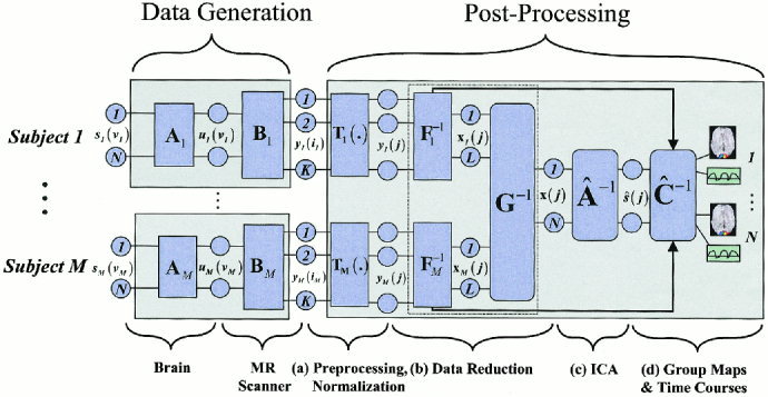
Model for the group ICA analysis. The model indicates our assumptions in the data‐generation block and our processing method in the postprocessing block. After spatial normalization and reduction, single subject data are combined together, followed by the independent component analysis, and finally individual subject maps and time courses are reconstructed and a “random effects” estimation is performed.

The first portion of the data generation block takes place within the brain. The second portion of the data generation block involves the fMRI scanner. We assume that K discrete time points were acquired with the scanner and that there are more time points acquired than there are sources in the brain. The sampling of the brain's hemodynamics with the fMRI scanner results in

(3)

where the fMRI data is discretely sampled in space (at locations indicated by i _p = 1, 2,…,V for the pth subject, where V is the number of voxels).

In the data processing block, we have a transformation T(.) representing a number of possible preprocessing stages, including slice phase correction, motion correction, spatial normalization, and smoothing. Following this stage, the effective spatial sampling for all subjects is indexed by j = 1, 2,…,M, so that we now have

(4)

To perform the group analysis, we make the assumption that the data collected from individual subjects are statistically independent observations. Thus, p _xy (x, y) = p _x (x) p _y (y), where p _i(i)|_i=x,y is a probability density function (pdf) of a source from subject i and p _xy (x, y) is the joint pdf for the same source for subjects x and y. Each subject is thus treated as an observation of the statistics of the population. Given this assumption, we will demonstrate that the unmixing matrix produced from the group ICA analysis will be largely separable across subjects.

The postprocessing block is the primary concern of this work. The stages of analysis include (a) preprocessing/spatial normalization, (b) data reduction, (c) estimation of independent components, and (d) thresholding/presentation of the results. The first stage (a) in our model involves preprocessing and spatial normalization of the data into a standard space [Talairach and Tournoux, 1988] followed by (b) data reduction. Two reduction steps, one on data from each subject (F̂ ₁ ⁻¹…F̂ _M ⁻¹) and one on an aggregate data set (Ĝ ⁻¹), are used to reduce the computational load of simply entering all subjects' data into an ICA analysis prior to reduction. In the third stage (c), estimation of independent sources is performed. The fourth stage (d) involves grouping components across subjects and thresholding the resulting group ICA images. The reasons for choosing this particular set of stages will become evident during the discussion of each of the three questions presented earlier.

How many components should be estimated?

The number of time points of the fMRI data has no relationship to the number of independent sources. In this method, we assume that there are more time points than sources in the fMRI scan, a reasonable assumption in many fMRI studies due to the large number of time points often acquired. Typically, principle component analysis (PCA) is used to represent most of the variance of the data (e.g., more that 99%) within a lower dimensionality [McKeown et al., 1998b] although other approaches to reduce the data, such as clustering [Calhoun et al., 2001a], can also be used. One could also choose to incorporate the data reduction into the ICA estimation stage directly. We chose to keep the data reduction as a separate stage because this seems a more natural way of treating the data and allows the estimation of the number of components.

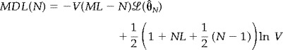
We propose using standard information theoretic methods for estimating the number of components from the aggregate data set. These methods make a decision based upon the complexity or information content of the data. The number of sources can be estimated using the well known Akaike's information criterion (AIC) or the minimum description length (MDL) criterion [Akaike, 1974; Rissanen, 1983]. These criteria have the following forms:

(5)

(6)

where V is the number of voxels, M is the number of subjects, £ (Θˆ_N) is the log of the maximum likelihood estimate of the model parameters (and is estimated from the data, e.g., fMRI data), ML is the number of time points following the first reduction stage, and N is the number of sources. The estimate for the number of sources is determined from the minima of the above functions with respect to N. These equations have been previously derived for a PCA decomposition resulting in the equation presented below

(7)

where λ_i represents the ith largest eigenvalue from the PCA decomposition [Karhunen et al., 1997; Wax and Kailath, 1985]. The expression for £ (Θˆ_N) is the ratio of the geometric mean of the LM‐N smallest PCA eigenvalues to their arithmetic mean. PCA is an optimal data reduction approach in that it minimizes the squared error associated with a lower dimensional set of orthogonal vectors. In the context of fMRI data, λ_LM represents the variance associated with the resultant best‐fit line through the fMRI data (consider a graph with LM axes, one per time point, and with one point plotted per voxel). The variance associated with the next best‐fit line (constrained to be orthogonal to the first line) is represented byλ_LM−1 continuing down toλ₁. The number of eigenvalues will be equal to the number of time points in the fMRI data set, although many of the smaller eigenvalues will be very close to zero.

The MDL criterion has the desirable property of statistical consistency, yielding asymptotically correct results [Karhunen et al., 1997; Wax and Kailath, 1985]. Although the AIC criterion does not have this theoretically desirable property, it may perform better at lower signal‐to‐noise ratios [Karhunen et al., 1997]. We thus chose to calculate both estimates and use the average of the two to determine the number of components.

HOW CAN COMPONENTS BE COMBINED ACROSS SUBJECTS?

We suggest entering all subjects into an ICA analysis and estimating one set of components. This has the advantage of ordering the components in different subjects in the same way. This produces a single set of “group” components that can then be interpreted. The estimation stage becomes computationally unwieldy for whole brain data sets, but the computational load can be decreased considerably by the incorporation of two data‐reduction stages as indicated. The data from the individual subjects are first reduced in dimension; these reduced data, from all subjects, are then concatenated (see Appendix). This data set is then further reduced resulting in a matrix that can be used in an ICA estimation stage.

The ICA maps from individual subjects are back‐reconstructed from the aggregate mixing matrix. A formal treatment of this process may be found in the Appendix; here we consider a heuristic case. Consider data in a voxel sampled at two time points from two subjects (subject x and subject y), d _x = [x ₁ x ₂] and d _y = [y ₁ y ₂], each of which is a normalized linear mixture of two hemodynamic sources. If we concatenate these subjects into a single vector, we have

(8)

Assuming the correct number of sources is two, the data reduction and ICA analysis result in a mixing matrix

(9)

and an estimate of the original sources ŝ = Wd where W is partitioned to depict the submatrices corresponding to the original mixed sources. To back‐reconstruct the individual subject maps we multiply the partition of W corresponding to the desired subject's data with the corresponding partition of d (e.g., s _x = W _x d _x).

Because the goal of ICA is to yield independent components, the rows of ŝ will be approximately statistically independent. Additionally, data from each subject is expected to be independent of each other. Then, we write the expression for ŝ

(10)

where we have defined s ₁₁ = α₁ x ₁ + α₂ x ₂, s ₂₁ = β₁ x ₁ +β₂ x ₂, s ₁₂ = α₃ y ₁ + α₄ y ₂, s ₂₂ = β₃ y ₁ + β₄ y ₂, and first note the statistical independence of s ₁₁ and s ₂₂ (and s ₁₂ and s ₂₁). Because the ICA algorithm minimizes the dependence among the signals (rows of ŝ), the dependence between s ₁₁ and s ₂₁ (and s ₁₂ and s ₂₂) will be minimized by more heavily relying on the data within that subject, forcing the parameters for each subject to be primarily determined by that subject's observations. Thus, the individual unmixing matrices will be approximately separable across subjects (partitions) and the back‐reconstructed data will be a function of primarily the data within subjects rather than across subjects.

In addition to the spatial maps, this analysis produces a representative time course, although this time course is not directly suitable for interpretation because it is derived from the reduced data sets. The unreduced fMRI time courses can be reconstructed by multiplying the dewhitening matrix from the first data reduction by the corresponding partition of W ⁻¹ (see Appendix). These time courses then reflect the hemodynamics of the fMRI experiment and may be inspected separately for each subject, or averaged across subjects to create a group time course.

How should the final results be thresholded?

We can threshold the resulting group ICA maps using a Z‐threshold criterion as suggested for single subject analysis [McKeown et al., 1998a]. Although this is a useful method, we suggest instead reconstructing single‐subject ICA maps from the group ICA estimation. As the ICA analysis produces estimates of hemodynamic sources, there is a physiologic meaning to the results. Thus, it makes sense to calculate the mean and variance of each component across subjects, where the variance across subjects can be used as an estimate of the population variance [Woods, 1996]. A hypothesis test can then be used to provide a “random effects” inference: the magnitudes or weights of the voxels within a set of ICA components are treated as random variables and a one‐sample t test with the null hypothesis of zero magnitude is performed.

EXPERIMENTS AND METHODS

Simulated experiment

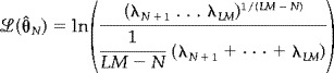
We apply these concepts to simulated data to illustrate their use. Two 30‐by‐30 spatial “sources” and associated 80‐point hemodynamic mixing time courses were generated (see Fig. 2). Each source was flattened into a 900‐element vector, and the two subsequently mixed by the hemodynamic time courses, resulting in a 900‐by‐80 matrix. Zero mean, Gaussian noise was then added to the mixed sources such that the contrast‐to‐noise ratio (CNR) for the largest simulated fMRI “activation” was 3.9, slightly less than half the CNR for our fMRI experiment. Nine sets of data, differing only in additive noise, were created to simulate a group of nine “subjects”. Each individual “subject” was first reduced from 80 time points to 20 time points using PCA, and the resulting data sets were concatenated together into an aggregate data set, resulting in a 900‐by‐180 matrix. The number of sources was then estimated from the aggregate data using AIC/MDL, and the aggregate data was further reduced using PCA to the dimension indicated by AIC/MDL, followed by independent component estimation. This yielded a set of aggregate components and time courses. The individual time courses and maps were then reconstructed and thresholded as described earlier.

Figure 2.

Simulated hemodynamic mixing functions (top), and spatial “sources” (bottom). Two sources were simulated; source 1 had 3 times the amplitude of source #2 as can be seen from the amplitudes of the hemodynamic mixing functions.

A second simulation was performed to determine how the sources that were back‐reconstructed from the aggregate mixing matrix would compare with sources that were generated from an ICA analysis performed separately on each “subject”. To determine this matrix, we simulated nine “subjects” as before, except eight of the nine subjects only had one source embedded within the data. The ninth subject had two sources (similar to the sources in the previous simulation). Noise was added to each data set as in the previous simulation. We then performed a group ICA analysis and calculated individual subjects maps from the aggregate mixing matrix. Additionally, we performed an ICA analysis on each subject individually and generated subjects' maps for comparison with the back‐reconstructed maps.

fMRI experiment

The Johns Hopkins Institutional Review Board approved the protocol and all participants provided informed consent. Data from nine normal subjects were acquired on a Philips 1.5T Scanner. Functional scans were acquired with an echo planar sequence (64 × 64, flip angle = 90, TR = 1 sec, TE = 39 msec) over a 6‐min period for a total of 360 time points. Nine slices were acquired, centered on the occipital pole and the frontal pole. A visual paradigm was presented in which an 8 Hz reversing black and white checkerboard was presented intermittently in the left and right visual fields for 30 sec at a time. The paradigm is depicted in Figure 3.

Figure 3.

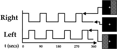
Paradigm used for the fMRI experiment. An 8 Hz reversing checkerboard was presented intermittently in the left and right visual fields. Subjects were instructed to maintain focus on a central crosshair during the 6‐min experiment.

Preprocessing

The images were first corrected for timing differences between the slices using windowed Fourier interpolation to minimize the dependence upon which reference slice is used [Calhoun et al., 2000; van de Moortele et al., 1997]. Next, the data were imported into the Statistical Parametric Mapping software package, SPM99 [Worsley and Friston, 1995]. Data were motion corrected, spatially smoothed with a 6 × 6 × 10 mm Gaussian kernel, and spatially normalized into the standard space of Talairach and Tournoux [1988]. The data were slightly subsampled to 3 × 3 × 4 mm, resulting in 53 × 63 × 34 voxels. For display here, slices 10–25 are presented.

General linear model

Data from each participant were used in a general linear model (GLM) analysis using SPM99 [Friston et al., 1996]. Regressors consisted of the two time courses (left visual field and right visual field) in Figure 3 convolved with an estimate of the hemodynamic response function. Data were high‐pass (drift removal) filtered by entering sinusoidal functions into the model up to a frequency of 1/180s as covariates and low‐pass filtered by smoothing the data temporally with a Gaussian kernel (4 sec full width at half maximum). These single‐subject maps were thresholded at p < .00001 [t = 4.5, degrees of freedom (df) = 79]. Additionally, a secondary “random effects” analysis was performed on the individual analyses by entering the amplitudes of the two regressors into a one‐sample t test. Results from this analysis were thresholded at p < .001 (t = 4.5, df = 8).

ICA

An AIC/MDL estimation on two subjects was performed, which predicted in both subjects fewer than 40 sources. Data from each subject were reduced from 360 time points to 40 time points using PCA. The results are not very sensitive to the reduction parameter; however, the original data should not be overly reduced to avoid losing important information. Data from all subjects were then concatenated and this aggregate data set was entered into an AIC/MDL estimation to determine the number of sources existing in the group data. The aggregate data were then reduced to this dimension using PCA, followed by an independent component estimation using an algorithm which attempts to minimize mutual information [Bell and Sejnowski, 1995]. Time courses and spatial maps were then reconstructed for each subject and the spatial maps were thresholded at p < .001 (t = 4.5, df = 8).

A question that arose was how performing the group ICA analysis and back‐reconstructing individual ICA maps from the aggregate mixing matrix would affect the individual mixing matrices. We thus performed a separate ICA analysis on each subject for comparison with the back‐reconstructed ICA maps. Data from each subject were reduced from 360 time points to 22 time points, a number greater than the intrinsic number of sources and less than the original dimensionality, using PCA and entered into an independent component estimation. Each resultant image was then converted to a Z score and thresholded at p < .00001 (Z = 4.23).

RESULTS

Simulated experiment

The number of sources in the simulated data set was correctly estimated to be two (see Fig. 4a). Group results from nine simulated “subjects” are shown in Figure 5. The group spatial maps (bottom) were thresholded at p < .001 (t = 4.5, df = 8), and match the actual sources very well. The amplitudes of the time courses were normalized to one. Note that there is increased variability in source #2 due to the lower amplitude of the hemodynamic mixing function. Having a hemodynamic mixing function, which is one‐third of that for source #1, is equivalent to an fMRI activation, which has one‐third of the amplitude of source #1 (refer to Fig. 2).

Figure 4.

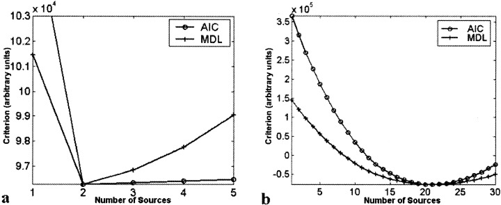
Results from AIC/MDL source estimation for (a) simulated, and (b) fMRI data. Both the AIC and MDL methods indicated the correct number of sources (2) for the simulated data set. For the fMRI data set, both AIC and MDL indicated 21 sources.

Figure 5.

Estimated sources and hemodynamic mixing functions. Results are thresholded at p > .001 (t = 4.5, dF = 8) with the regions that surpassed the threshold outlined in red. Both sources are correctly identified. Note that source #2 had a higher degree of variability (both in the time course and in the spatial map) due to the lower amplitude of the original source.

Results from our second simulation are presented in Figure 6. ICA spatial maps generated from individual subjects were very similar to spatial maps back‐reconstructed from the aggregate mixing matrix.

Figure 6.

Comparison of (a and c) individual ICA maps with (b and d) back‐reconstructed ICA maps. Note that one of the nine “subjects” had two sources, both of which are successfully detected by the back‐reconstructed ICA maps and the individual ICA maps. Eight of the subjects only had one source, thus the maps for source #2 are just noise. Overall, the two methods yielded similar results.

fMRI experiment

Single‐subject results from the fMRI experiments are presented in Figure 7 for the (a) general linear model, (b) back‐reconstructed ICA, and (c) individual ICA methods for slice 15 of the spatially normalized data. Results are overlaid onto the normalized EPI images from the appropriate subjects. The GLM results are thresholded at p < .00001 (t = 4.5, df = 79), and the ICA results are thresholded at p < .00001 (Z = 4.23). Twenty‐one components were estimated for the ICA results; two task‐related components (depicted in red and blue, respectively) along with one transiently task‐related component (depicted in green) are presented in the figure. Note that the GLM maps seem quite similar to the ICA maps for the task‐related components. The back‐reconstructed ICA maps seem similar to the ICA maps performed on individual subjects. Note that there are some differences between the maps at the chosen threshold, but when applying a slightly lower threshold (not shown) the overall similarity of the two sets of ICA maps is confirmed.

Figure 7.

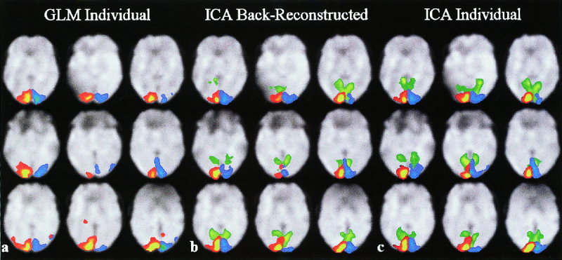
(a) Single subject results for GLM, (b) back‐reconstructed ICA, and (c) individual ICA. A single slice is presented for each of the nine subjects depicting activation significantly activated when the right (red) and left (blue) visual fields were stimulated. A transiently task‐related component located in the visual cortex is also depicted on the ICA images (green).

Group maps for both the GLM and ICA analyses are presented in Figure 8. The number of components was estimated to be 21 by both MDL and AIC, so the aggregate data were reduced to this dimension and 21 components were estimated. Both maps are thresholded at p < .001 (t = 4.5, df = 8). Group ICA maps resembled individual subject maps but were considerably smoother (compare to the group maps produced using SPM99). There were several interesting components within the data (see Fig. 8c). Separate components for primary visual areas on the left and the right visual cortex (depicted in red and blue, respectively) were consistently task‐related with respect to the appropriate stimulus. A large region (depicted in green) including occipital areas and extending into parietal areas seemed to be deactivated when the visual stimuli from either hemi‐field was turned off. This area follows the parieto‐occipital sulcus upward and extends on both sides, including portions of cuneous, precuneous, and the lingual gyrus. Additionally, we identified visual association areas (depicted in white) that were consistently detected across the group of subject; however, the time courses were not task‐related.

Figure 8.

Random effects group fMRI results for (a) GLM, and (b) ICA, both thresholded at p < .001 (t = 4.5, df = 8). Five components are presented including task‐related components in right visual cortex (red), left visual cortex (blue); a transiently task‐related component (TTR, green) in bilateral occipital/parietal cortex; and non‐task‐related components in bilateral visual association cortex (NTRV, white outline) and primary auditory cortex (NTRA, pink). (c) Time courses for the components are presented. Standard deviation across the group of nine subjects is indicated for each time course with dotted lines.

DISCUSSION

We have presented a method for making group inference maps through the application of independent component analysis to fMRI data. We have applied it to a simple visual paradigm and identified several distinct visual areas, which were either consistently task‐related, transiently task‐related, or correlated but non‐task‐related. Among these, we identified bilateral occipital/parietal areas, which indicated transient decreases only when the visual stimuli from either eye were turned off. The visual areas that were not task‐related may have been detected because of functional connectivity. This is related to experiments in which correlations are detected between functionally related regions [Biswal et al., 1995] and also agrees with the fact that bilateral primary auditory cortex (see Fig. 7) and other areas (not shown) are consistently detected in our ICA studies.

A few comments on the particulars of our method are in order. It is important to consider how the preprocessing stages affect the resulting images. The preprocessing stages performed include timing correction, motion correction, spatial normalization, and smoothing. The first three are necessary to attempt to place the image data from all subjects into the same point of reference in both time and space. The smoothing is useful as it both reduces the amount of high‐frequency spatial noise as well as desensitizes the images to errors in the motion correction and normalization. It is straightforward to demonstrate that spatial smoothing will not affect the (spatial) ICA estimate (i.e., the mixing matrix will be the same though the source maps will be smoothed) and thus is a reasonable preprocessing step [Hyvarinen and Oja, 2000].

In Figure 8, it is interesting to note that at the same threshold, the group ICA maps indicate greater spatial extent of activation than the group SPM maps for both the left and the right visual field stimulation. The SPM group results were generated by performing a t test on the amplitudes resulting from a GLM estimation (tested against a null hypothesis of zero amplitude). We chose such a comparison because testing the amplitudes in a GLM analysis is the more common approach due to the physiologic meaning of the amplitude estimates [Holmes and Friston, 1998]. However, we also performed a t test on the individual SPM{t} maps (not shown), and the resulting maps are very similar in spatial extent to the depicted GLM results. The ICA t test also has physiologic meaning, as our initial assumption was that the ICA maps represent statistically independent hemodynamic sources in the brain.

We chose to estimate the number of sources present from the fMRI data itself. Order selection, however, is not an easy problem, and such methods are often largely empirical in nature. We chose the number of components to provide a good tradeoff between preserving much of the information in the data while reducing the size of the data set, thus making the ICA computation and interpretation less intensive. We have presented one approach to determine the optimal reduction parameter, but it should be noted that order selection methods are still an area of active investigation. The use of our Group ICA method, however, may improve the statistics used for order selection methods due to the increase in sample points. It thus might be more useful to perform such estimations on group‐averaged data.

Starting from the assumption that data from subjects represent independent observations, we have demonstrated that the aggregate mixing matrix is separable across subjects. Empirically, we have demonstrated, both for simulated data and for fMRI data, that doing an ICA analysis on individual subjects ends up yielding largely similar results to performing an aggregate analysis. However, an alternative, which does not make this assumption yet still provides for group inference, is recombining an ICA analysis performed on each subject individually (as one would do for a single‐subject analysis). A set of N _i components is produced for each subject, and the challenge is then to determine how to combine these components across the subject. We have explored methods for performing this combination automatically and have previously used a manual combination method [Calhoun et al., 2001c]. Additionally, one could choose to perform a group analysis as we have done in this work as well as an individual ICA analysis. The individual back‐reconstructed ICA maps could then be used as a template with which to order and combine the ICA maps from the individual ICA analysis (by calculating the correlation of the individual maps with the group ICA maps and sorting them by correlation coefficient). Of these possibilities, the group method we present in this work provides the least amount of both computation time and manual interpretation.

Future studies

There is some evidence that the visual areas detected are related to the task in general, as they are not detected in ICA analysis of data from experiments in which a different task is performed (e.g., a visual perception task) [Calhoun et al., 2001c]. Interpretation of non‐task‐related regions is difficult, but may be possible with carefully designed control tasks and additional studies of the properties of ICA decomposition of fMRI. Additionally, methods related to hybrid ICA might be useful in understanding how to interpret non‐task‐related regions [McKeown, 2000].

Registration errors do not seem to be a significant problem in our experiment, which involved very striking changes in the left and right visual cortices that could be easily inspected. However, ICA of paradigms involving subtler changes or transiently task‐related components may require further investigation into the effects of these stages.

In conclusion, we have extended independent component analysis of fMRI data to provide for group inferences. Our method has general applicability, is straightforward to apply, and should be computationally reasonable for many fMRI group studies.

DATA REDUCTION AND SINGLE‐SUBJECT PARTITIONING

Data reduction

Let X _i = F _i ⁻¹ Y _i be the L‐by‐V reduced data matrix from subject i, where Y _i is the K‐by‐V data matrix (containing the preprocessed and spatially normalized data), F _i ⁻¹ is the L‐by‐K reducing matrix (determined by the PCA decomposition), V is the number of voxels, K is the number of fMRI time points, and L is the size of the time dimension following reduction. Note that all inverses are considered to be psuedoinverses if the matrix is not square.

The next step is to concatenate the reduced data from all subjects into a matrix and reduce this matrix to N (the number of components to be estimated). The N‐by‐V reduced, concatenated matrix for the M subjects is

(A1)

where G ⁻¹ is an N‐by‐LM reducing matrix (also determined by a PCA decomposition) and is multiplied on the right by the LM‐by‐V concatenated data matrix for the M subjects.

ICA estimation

Following ICA estimation, we can write X =  Ŝ, where  is the N‐by‐N mixing matrix and Ŝ is the N‐by‐V component map. Substituting this expression for X into Equation (A1) and multiplying both sides by G, we have

(A2)

Partitioning

Partitioning the matrix G Â by subject provides the following expression

(A3)

We then write the equation for subject i by working only with the elements in partition i of the above matrices such that

(A4)

The matrix Ŝ _i in Equation (A4) contains the single subject maps for subject i and is calculated from

(A5)

Single‐subject maps and time courses

We now multiply both sides of Equation (A4) by F _i and write

(A6)

which provides the ICA decomposition of the data from subject i, contained in the matrix Y _i. The N‐by‐V matrix Ŝ _i contains the N source maps and the K‐by‐N matrix F _i G _i  _i is the single subject mixing matrix and contains the time course for each of the N components.

REFERENCES

- Akaike H (1974): A new look at statistical model identification. IEEE Trans Automatic Control 19: 716–723. [Google Scholar]
- Bell AJ, Sejnowski TJ (1995): An information maximisation approach to blind separation and blind deconvolution. Neural Computation 7: 1129–1159. [DOI] [PubMed] [Google Scholar]
- Biswal B, Yetkin FZ, Haughton VM, Hyde JS (1995): Functional connectivity in the motor cortex of resting human brain using echo‐planar MRI. Mag Res Med 34: 537–541. [DOI] [PubMed] [Google Scholar]
- Biswal BB, Ulmer JL (1999): Blind source separation of multiple signal sources of FMRI data sets using independent component analysis. J Comput Assist Tomogr 23: 265–271. [DOI] [PubMed] [Google Scholar]
- Calhoun V, Golay X, Pearlson G (2000): Improved FMRI slice timing correction: interpolation errors and wrap around effects. Proceedings, ISMRM, 9th Annual Meeting, Denver.
- Calhoun V, Adali T, Pearlson G (2001a): Independent components analysis applied to FMRI data: a natural model and order selection. Proceedings, NSIP, Baltimore.
- Calhoun V, Adali T, Pearlson G Pekar J (2001b): Spatial and temporal independent component analysis of functional MRI data containing a pair of task‐related waveforms. Hum Brain Mapp 13. [DOI] [PMC free article] [PubMed] [Google Scholar]
- Calhoun V, Pekar J, Adali T, Pearlson G (2001c): FMRI of visual perception: networks identified by SPM and independent component analysis. Proceedings, ISMRM, 10th Annual Meeting, Glascow, Scotland.
- Friston KJ, Holmes A, Poline JB, Price CJ, Frith CD (1996): Detecting activations in PET and FMRI: levels of inference and power. Neuroimage 4: 223–235. [DOI] [PubMed] [Google Scholar]
- Holmes AP, Friston KJ (1998): Generalizability, random effects, and population inference. Neuroimage 7: S754. [Google Scholar]
- Hyvarinen A, Oja E (2000): Independent component analysis: algorithms and applications. Neural Net 13: 411–430. [DOI] [PubMed] [Google Scholar]
- Karhunen J, Cichocki A, Kasprzak W, Pajunen P (1997): On neural blind separation with noise suppression and redundancy reduction. Int J Neural Syst 8: 219–237. [DOI] [PubMed] [Google Scholar]
- McKeown MJ (2000): Detection of consistently task‐related activations in FMRI data with hybrid independent component analysis. Neuroimage 11: 24–35. [DOI] [PubMed] [Google Scholar]
- McKeown MJ, Sejnowski TJ (1998): Independent component analysis of FMRI data: examining the assumptions. Hum Brain Mapp 6: 368–372. [DOI] [PMC free article] [PubMed] [Google Scholar]
- McKeown MJ, Jung TP, Makeig S, Brown G, Kindermann SS, Lee TW, Sejnowski TJ (1998a): Spatially independent activity patterns in functional MRI data during the Stroop color‐naming task. Proc Natl Acad Sci 95: 803–810. [DOI] [PMC free article] [PubMed] [Google Scholar]
- McKeown MJ, Makeig S, Brown GG, Jung TP, Kindermann SS, Bell AJ, Sejnowski TJ (1998b): Analysis of FMRI data by blind separation into independent spatial components. Hum Brain Mapp 6: 160–188. [DOI] [PMC free article] [PubMed] [Google Scholar]
- Rissanen J (1983): A universal prior for integers and estimation by minimum description length. Ann Statistics 11: 416–431. [Google Scholar]
- Talairach J, Tournoux P (1988): A co‐planar sterotaxic atlas of a human brain. Stuttgart: Thieme. [Google Scholar]
- van de Moortele PF, Cerf B, Lobel E, Paradis AL, Faurion A, Le Bihan D (1997): Latencies in FMRI time‐series: effect of slice acquisition order and perception. NMR Biomed 10: 230–236. [DOI] [PubMed] [Google Scholar]
- Wax M, Kailath T (1985): Detection of signals by information theoretic criteria. IEEE Trans Acoust Speech, Sig Proc 33: 387–392. [Google Scholar]
- Woods RP (1996): Modeling for intergroup comparisons of imaging data. Neuroimage 4: S84–S94. [DOI] [PubMed] [Google Scholar]
- Worsley KJ, Friston KJ (1995): Analysis of FMRI time‐series revisited—again. Neuroimage 2: 173–181. [DOI] [PubMed] [Google Scholar]