

Abstract
The major disadvantage of hierarchical clustering in fMRI data analysis is that an appropriate clustering threshold needs to be specified. Upon grouping data into a hierarchical tree, clusters are identified either by specifying their number or by choosing an appropriate inconsistency coefficient. Since the number of clusters present in the data is not known beforehand, even a slight variation of the inconsistency coefficient can significantly affect the results. To address these limitations, the dendrogram sharpening method, combined with a hierarchical clustering algorithm, is used in this work to identify modality regions, which are, in essence, areas of activation in the human brain during an fMRI experiment. The objective of the algorithm is to remove data from the low‐density regions in order to obtain a clearer representation of the data structure. Once cluster cores are identified, the classification algorithm is run on voxels, set aside during sharpening, attempting to reassign them to the detected groups. When applied to a paced motor paradigm, task‐related activations in the motor cortex are detected. In order to evaluate the performance of the algorithm, the obtained clusters are compared to standard activation maps where the expected hemodynamic response function is specified as a regressor. The obtained patterns of both methods have a high concordance (correlation coefficient = 0.91). Furthermore, the dependence of the clustering results on the sharpening parameters is investigated and recommendations on the appropriate choice of these variables are offered. Hum. Brain Mapping 20:201–219, 2003. © 2003 Wiley‐Liss, Inc.
Keywords: fMRI, hierarchical clustering, dendrogram sharpening, single link
INTRODUCTION
Data analysis techniques in fMRI can be loosely classified into two categories: model‐dependent and model‐free methods. The first category encompasses standard statistical approaches such as Statistical Parametric Mapping (SPM) (Wellcome Department of Cognitive Neurology, London, UK), where the hemodynamic response function is explicitly modeled. However, their use is limited in studies with more complex activation paradigms or unknown brain response patterns (e.g., drug studies, epileptic seizures, or analysis of resting‐state data). To identify unknown brain responses, exploratory methods such as principal component analysis (PCA) [Sychra et al., 1994], independent component analysis (ICA) [McKeown et al., 1998], and cluster analysis are useful. The most popular methods among the numerous clustering techniques are fuzzy clustering [Baumgartner et al., 1998, 2000a, b; Windischberger et al., 2001] and K‐means [Goutte et al., 1999]. Even though fuzzy and K‐means clustering are regarded as exploratory, data‐driven methods, they still require the specification of the number of expected clusters.
Hierarchical clustering methods have been successfully applied to fMRI data [Cordes et al., 2002; Filzmoser et al., 1999; Goutte et al., 1999]. Hierarchical clustering, contrary to K‐means, is not based on a multivariate Gaussian distribution of the data, and has therefore advantages in classifying various types of distributions. The aim of any clustering method in fMRI is to create a partition of the entire data set into distinct regions where each region is represented by voxels exhibiting similar temporal behavior. One of the obstacles in fMRI data analysis is the large size and complexity of the raw data set, the low contrast‐to‐noise ratio (CNR), and the presence of artifacts including subject motion and hardware instabilities. The ultimate goal is to detect areas of real activation. Hierarchical clustering allures with its simplicity and its absence of any underlying parametric assumptions. One only needs to specify the measure of similarity, which is then used to link the objects into a binary tree. The clusters are usually defined by setting an appropriate inconsistency threshold, which is equivalent to a cut of the binary tree at a certain level. However, due to the presence of noise in the fMRI data, this “cutting” method can result in any arbitrary number of clusters.
The purpose of this study is to evaluate the application of a particular sharpening algorithm to obtain robust activation maps. The sharpening technique, in general, allows a significant reduction of the dimensionality of the acquired data, at the same time preserving its structure. In the present study, two different on/off motor paradigms, a slow‐paced and a fast‐paced finger tapping experiments, are used. The correlation coefficient between two voxel time courses serves as a measure of similarity. The choice of the appropriate linking method is discussed. To evaluate clustering results, the performance of the algorithm is compared to the outcome of a conventional statistical analysis using a hypothesized hemodynamic response function as a regressor. Finally, the dependence of the obtained clusters on the sharpening parameters is investigated and suggestions for the appropriate values choice are given.
THEORY
Distance Measure
The first step in clustering is to define a distance measure between the objects (points), d(i,j). This measure must satisfy the following three properties:
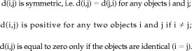 |
The defined measure is a metric if in addition to the listed properties the triangle inequality is satisfied:
The choice of the similarity measure depends on the data type (nominal, ordinal, ratio, etc.) and the accepted practice in the application field. Common examples of similarity measures include Euclidian and Mahalanobis distances. A detailed description and discussion of possible similarity measures are beyond the scope of this study and can be found elsewhere [Hartigan, 1981; Jain and Dubes, 1988].
Linkage Algorithm
Cluster linking is accomplished by grouping the acquired data into a hierarchical tree using an appropriate linkage method. The three most popular and basic linkage methods in hierarchical agglomerative clustering are the single link, complete link, and average link method. All these methods lead to a binary tree called a dendrogram that describes the structure of the data. In the single linkage method (also called the nearest neighbor method), the distance between two clusters is defined as the minimum of all pairwise distances between objects constituting the clusters. At each step, the two closest clusters are joined together. Complete linkage, or “furthest neighbor linkage,” in turn, uses the largest distance between objects to separate two clusters. The average linkage method uses the average distance between all pairs of objects from two different clusters.
For completeness, we like to mention briefly the popular K‐means algorithm, which is an example of a partitioning algorithm. It aims to partition the data into distinct groups by minimizing the sum of distances from each object to its cluster centroid over all clusters. For more information on clustering algorithm, the reader is referred to Hartigan [ 1975] and Jain and Dubes [ 1988].
Terminology
Next we review some of the basic terminology used in hierarchical clustering. The original data points are referred to as terminal nodes. When two nodes are merged together they form a new node, called a parent node. When the last two clusters are merged together they form a root node. The ordinate value of a parent node on the diagram is equal to the distance between the objects forming the node. This distance is also called agglomeration value. The two nodes agglomerated to form a new cluster are called left and right child of the newly formed cluster, respectively. The size of the particular node equals the number of the terminal children constituting the node. Obviously the size of any terminal node is one and the size of the root node (i.e., the top node) is equal to the number of the terminal children.
Advantages of Using the Single Linkage Method
Here, the single linkage method is used because of its ability to correctly reveal the underlying structure of the data. This is not necessarily the case for the other linkage methods, unless points of high density are separated by a sufficiently deep valley of zero density. For example, when sets of original points become close or overlap, the complete and average linkage algorithms yield several large clusters, giving an impression of distinct grouping in the data regardless of the density. It has been shown [Hartigan, 1981] that the large clusters produced by these algorithms depend on the range, but not on the true density of the data set. Thus, complete and average linkage algorithms are unable to properly indicate the modal peaks unless the data is constituted of well‐separated groups of objects. Single linkage behaves differently, producing long chained clusters that are difficult to interpret. Many top nodes of the single linkage dendrogram have a very small and a sufficiently large child. Due to this “chaining” effect, which correctly indicates the lack of spatial separation in case of touching or overlapping clusters, the single linkage has been neglected by many researchers.
Hartigan [ 1975, 1977a, b, 1981] provides formal support for the usage of the single linkage over average and complete linkage algorithms. Hartigan shows that single linkage is fully consistent for separating two disjoint, high‐density clusters in R n when n =1, and that it is fractionally consistent for n > 1. The latter case means that if two disjoint population groups exist, there will be two distinct single linkage clusters containing a positive fraction of the sample points from the corresponding population groups. It then follows that the single linkage is in a sense conservative, that it won't necessarily detect all clusters, but it will detect modal regions separated by a sufficiently deep valley [Hartigan, 1977b].
The single linkage has other alluring properties: it is computationally simple, it produces clusters invariant under reordering of the objects, and it is related to the minimum spanning tree (MST). The MST is the graph of minimum length connecting all data points. An example of the MST is given below.
Example
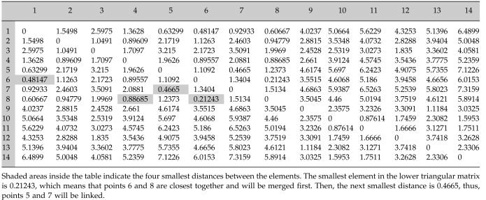
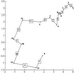
To gain a better understanding, consider the following example of the single linkage algorithm for a small data set consisting of fourteen points in R 2 labeled from 1 to 14 (Fig. 1). Initially, every point is a cluster. The first step is to compute all pairwise distances between the points. In this example, the distance is defined as the simple Euclidean distance in R 2 . Due to the discussed distance properties, the distance matrix d(i,j) (Table I) is symmetric with zeros on the main diagonal. Consider the lower triangle matrix and find its smallest element. This element is d(8,6) and means that the points 6 and 8 are closest together. These will be merged to form a new cluster 15. At the next step, points 5 and 7 represent the closest clusters and will be linked together to form object 16. The next smallest value of the distance matrix is d(6,1). But object 6 already formed the new cluster 15, thus object 1 will be combined with cluster 15 to form a new node 17. The process continues until all nodes merge to a single cluster. Table II shows a step‐by‐step linking process. The first column represents a new parent cluster formed by merging together clusters from the second and third columns of the corresponding row. The last column shows the distance between the linked objects. The result of this process is the single linkage dendrogram (SLD) shown in Figure 2. The original 14 objects are marked on the horizontal axis. Clusters created during the linking process are marked as black points on the diagram and labeled from 15 to 27. It is quite obvious that in order to connect n objects one needs to make (n‐1) links, thus, it will take 13 edges to connect 14 vertexes. Referring to our terminology, the node 27 is the root node of the dendrogram and has a size of 14. Consider, for instance, node 22. Its left child will be node 21, its right child node 3. The agglomeration value of node 22, that is the distance between cluster 21 and 3, is about 1.05. The size of node 22 is 8, because it has eight terminal children {6,8,1,5,7,4,2,3}.
Figure 1.
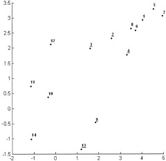
Simulated two‐dimensional Gaussian cloud consisting of 14 points labeled by consecutive integers. Objects that are discarded later by sharpening are underlined.
Table I.
Matrix of Euclidian distances for the simulated data set in Figure 1
|
Table II.
Linkage process for the simulated data set in Figure 1
| Parent node | Left child | Right child | Distance |
|---|---|---|---|
| 15 | 6 | 8 | 0.21243 |
| 16 | 5 | 7 | 0.4665 |
| 17 | 1 | 15 | 0.48147 |
| 18 | 17 | 16 | 0.63299 |
| 19 | 10 | 11 | 0.87614 |
| 20 | 18 | 4 | 0.88685 |
| 21 | 20 | 2 | 0.89609 |
| 22 | 21 | 3 | 1.0491 |
| 23 | 9 | 13 | 11.1184 |
| 24 | 19 | 14 | 1.5953 |
| 25 | 24 | 12 | 1.6666 |
| 26 | 22 | 25 | 1.835 |
| 27 | 26 | 23 | 2.3082 |
Objects in column 1 are formed when objects in columns 2 and 3 in the corresponding row are linked together. Column 4 lists distances between the linked objects.
Figure 2.
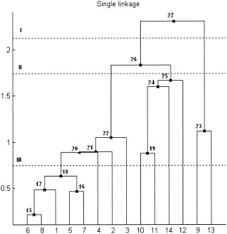
Single linkage dendrogram for the simulated data set. Values on the horizontal axis are points from the initial data set numbered from 1 to 14. Black nodes and numbers on the dendrogram tree represent the internal nodes formed by the linkage algorithm. Values on the vertical axis are the distances between combined objects.
The MST is constructed as follows (Fig. 3): the two closest observations (6 and 8) are connected by edge 1 (the edge numbers are given in the diagram in squares). The next two closest points, 5 and 7, are connected by edge 2 and so on. To complete the MST, the objects will be connected in exactly the same order as for the SLD.
Figure 3.
Minimal Spanning Tree (MST) of the data from Figure 1. Numbers in squares indicate the edges of the tree.
The single linkage clusters can be obtained from the MST by a number of methods. For example, removing one of the edges of the MST will split the set into two connected subsets representing two distinct clusters. This operation on the MST is equivalent to the incision of the dendrogram tree at the corresponding level. Returning to the previous example (Fig. 3), deleting the largest edge 13 will yield two subsets. The first subset contains two points {9,13}, and the second consists of all the remaining 12 objects. The same data set division could be obtained by cutting the binary tree at level one (Fig. 2, dashed line I). Removing the second largest edge 12 from the MST yields three clusters {9,13}, {10,11,14,12}, and {6,8,1,5,7,4,2,3}. Exactly the same grouping could be obtained by cutting the SLD at level II and so on. All the single‐linkage clusters could be obtained by deleting the edges of the MST, starting from the largest one.
The Dendrogram Sharpening Algorithm
Finding natural divisions in the data set is a challenging task. The ideal situation is where the population clusters are separated by a deep valley of zero density. In practice, in a large data set the observations in the tails contaminate the picture, filling the space between the modal peaks. The known solution to this problem is to alter the original collection of objects in order to reveal its underlying structure. One natural alteration is to sharpen the data to increase the contrast between the density regions. The goal of this procedure is to reduce the number of considered elements, by deleting or by agglomerating them, and at the same time preserving as much structure of the data as possible.
Sharpening could be performed by a number of ways. In sharpening by excision, observations in regions of low density are simply deleted. However, this sharpening method has one serious disadvantage. If the original data consist of groups of different densities, there is a great risk that the smallest clusters will be completely removed. In sharpening by replacement, each point is replaced by the centroid of it and its nearest neighbors. More details on sharpening techniques can be found in Tukey and Tukey [ 1981]. In this work, the dendrogram sharpening algorithm introduced in McKinney [ 1995] is applied. The idea of the algorithm is to discard all small‐sized children‐nodes with a large‐sized parent node in the dendrogram tree. As it was indicated [McKinney, 1995], this technique yielded consistently good results, correctly reflecting the multimodal structure of the data by well‐separated clusters in the sharpened set.
Formally, our sharpening process is controlled by two parameters, nfluff and ncore The nfluff value is the maximum size of a child cluster that will be discarded if it has a parent node of a size larger than ncore. This is a recursive algorithm that begins with the root node of the dendrogram and continues to invoke on the children of each node since each child node is the root node of a dendrogram tree itself. This is described by a flowchart in Figure 4. Different values of the sharpening parameters together with simple or multiple passes over the data yield a variety of sharpening effects.
Figure 4.
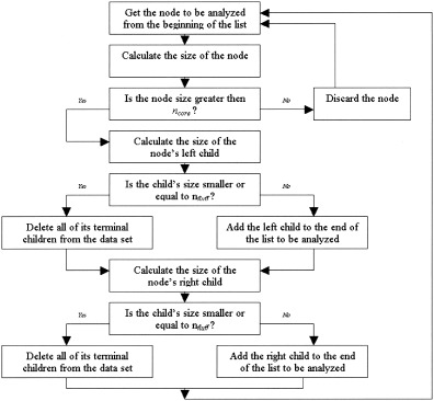
The Dendrogram Sharpening Algorithm.
Consider a simple example of the sharpening technique. Recall the very first example (Figs. 1, 2, 3) where 14 points were linked together into a hierarchical tree using the single linkage method based on the conventional Euclidian distance. The dendrogram sharpening algorithm will be applied to the SLD (Fig. 2) with (nfluff, ncore) parameters (2,5), which means that from every node of a size larger than 5, all its children of a size smaller or equal 2 will be discarded. The procedure starts from the root node of the tree 27. Its size equals the number of the terminal nodes that is 14. Since 14 is greater than 5, the root node is subject to sharpening. It has two children: the left child 26 has a size of 12 and the right child 23 has a size of 2. Further on, the size of the node will be indicated as a number in parenthesis. Node 23 will be discarded because its size satisfies the original condition: 2 ≤ 2. The size of the left child 26 (12) is greater than 2 so it will remain unchanged and will be the next node to be analyzed. The children of node 26 are node 22 (8) and node 25 (4). Both of them remain unaltered since they are of a size greater than 2. The size of node 22 (8) is greater than 5 and thus this root will be analyzed next. Because the size of the right child 25 (4) is less than 5, it no longer satisfies the sharpening conditions, so all its four terminal nodes {10,11,14,12} will be listed in the sharpened data set. The left child 22 (8) will be sharpened in a similar manner. It is obvious from the diagram that the right single‐point children of nodes 22,21,20 will be discarded. Node 18 (5) will remain unchanged because its size is not larger than 5. Thus, points {4,2,3,9,13} are excluded by sharpening. Using the single linkage method to join the remaining nine points will produce a new SLD of the sharpened data (Fig. 5) that clearly reveals the presence of the two distinct groups in the data set. Objects {3,5,1,2,4} on the sharpened SLD correspond to objects {6,8,1,5,7} from the original data set and form one cluster. Points {6,7,9,8}, which are in fact the objects {10,11,14,12} from the original data, constitute the second cluster. Since the original fourteen points of the data set consisted of two Gaussian clusters in R 2 (set {1,…,8} and set {9,…,14}, respectively), it is interesting to note two facts. One is that the discarded objects {4,2,3,9,13} represent the outliers in each of the two clouds (Fig. 1, see the underlined points), and, two, sharpening not only correctly indicates the bimodality of the data, but also properly classifies the objects between the two groups.
Figure 5.
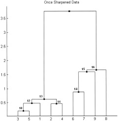
Dendrogram tree after single sharpening of the data in Figure 1 (see the original SLD tree on Fig. 2 to follow up the sharpening process). Resulting tree clearly indicates the presence of two distinct clusters in the data. The first cluster {3,5,1,2,4} corresponds to points {6,8,1,5,7} from the original data set. The second cluster {6,7,8,9} is essentially the objects {10,11,14,12}.
However, before applying the sharpening algorithm to the fMRI data, a slight adjustment will be made to avoid the following problem. As it was indicated, the sharpening algorithm depends only on two parameters, namely the size of a node and the size of its children. Suppose sharpening is performed with parameters nfluff = 2, ncore = 5 on the dendrogram tree, shown in Figure 6. Then the left child, encircled in the diagram, will be discarded and all the terminal nodes of the right child will be present in the sharpened data. Obviously, the voxels that are closest to each other will be eliminated, and pixels that are further apart will remain in the altered data set. To eliminate this problem, the algorithm was slightly modified. If a particular child is subject to sharpening, it will be deleted only when its agglomeration value is larger than that of the remaining child. Thus, in case of the illustrated example (Fig. 6), all six terminal nodes will be present in the sharpened data set. The modified algorithm preserves a larger number of data points and gives a researcher a better insight into the structure of the data in the early stage of an investigation.
Figure 6.
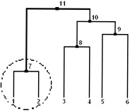
Example of the “problematic” single linkage tree. If sharpening with parameters nfluff = 2 and ncore = 5 is performed on the data linked to form this tree, the encircled child will be discarded even though it is formed of the two closest objects from the entire data set.
Cluster Identification
Cluster identification begins upon the completion of the sharpening. One way to detect the natural grouping of the data is to compare the length of each link in a cluster tree with the length of neighboring links below it in the tree. If the length of the link does not differ significantly from the length of the neighboring links, it means that objects, joined at this level of the hierarchy, have similar characteristics. Otherwise, when the length of the link is much larger than the length of the neighboring links, it indicates some dissimilarity between the objects, and this link is said to be inconsistent.
In this report, the method of inconsistent edges [McKinney, 1995] is used to identify cluster cores. This algorithm exploits the correspondence between the SLD and the MST. The length of the edge in the MST is an agglomeration value of the corresponding node in the SLD. Because the two objects joined at the particular level of hierarchy could have different densities, the length of the edge connecting them should be compared to the length of the edges represented by the left child and by the right child separately. The value of the median edge length of the left (right) subtree plus twice the interhinge spread (described below) is the proposed threshold, beyond which the edge is considered inconsistent with respect to its left (right) child. Mathematically, this threshold, T, is given by
| (1) |
where M r(l), U r(l) and L r(l) are the median, upper‐, and lower‐hinge values of the set of the agglomeration values constituting the right(left) child, respectively. The upper hinge and lower hinge [Tukey, 1977] correspond to the first and third quartile of the ordered data, respectively. The interhinge spread, that is the difference between the upper and lower hinge, gives a robust measure of spread of the edge lengths. The recursive procedure begins with analyzing the root node of the SLD and then invokes on its children.
Final Classification
After clusters in the sharpened data are identified, the voxels that have been set aside during sharpening can be reclassified in order to reassign them to the obtained cores. At this step, the linkage matrix, built for the original data, has to be recalled. The unclassified voxels are assigned to the cluster group, to which they are joined by the link of minimal length. This is a bottom‐up algorithm. Initially, each data point represents a cluster. Thus, every cluster has all members classified or unclassified. If two clusters, linked together, are either classified or unclassified, they are simply merged together forming a new cluster that has all of its members classified or unclassified, respectively. If the classified cluster is linked together with the unclassified cluster, the point in the classified cluster closest to the unclassified cluster is found. All data points in the unclassified cluster are assigned to the group of which the found point is a member [McKinney, 1995].
Simulation
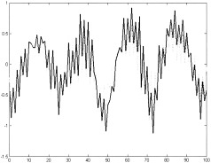
In the following, we show how the single, average, and complete linkage algorithms behave for unimodal and bimodal Gaussian distributed data. Consider a simulated Gaussian cloud plotted in Figure 7A. Plots (Fig. 7B–D) show three dendrograms constructed using single, average, and complete linkage, respectively. Average and complete linkage trees suggest the presence of few distinct clusters in the data set. Single linkage, in turn, produces long chained clusters indicating the lack of spatial separation between the objects. After applying the dendrogram sharpening once (Fig. 7E) and twice (Figure 7F), the SLD becomes more structured. But the method of inconsistent edges does not identify any well‐separated clusters in the data and classifies all the data points as members of the same family.
Figure 7.
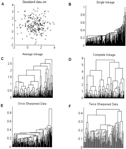
Scatter plot of a simulated Gaussian cloud (A); dendrograms for the (B) single, (C) average, (D) complete linkage; dendrogram of the once (E) and twice (F) sharpened data set. Average and complete linkage tree indicate incorrectly that the data set is well structured and contains at least two separate clusters. Single linkage dendrograms of the raw and once‐sharpened data exhibit lack of spatial separation between the points in the data set, which is correct. Though the tree of the twice‐sharpened data reveals certain structure, the method of inconsistent edges does not identify any clusters.
In another simulation, Figure 8A shows two overlapping Gaussian clouds plotted using different markers. Again, the single linkage detects objects that are closest to each other and then simply connects the remaining outliers to the cluster core exhibiting a strong “chaining” effect. After passing the sharpening algorithm over the data twice, the tree becomes more structured (Fig. 8E,F) and the method of inconsistent edges indicates the presence of two clusters in the original data set. Since the natural division in the simulated data set is known, it is possible to manually classify the remaining objects. Points of the reduced data set are plotted in Figure 8G using two different markers.
Figure 8.
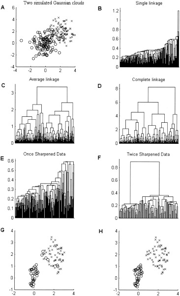
A: Two overlapping Gaussian clouds; dendrograms for the (B) single, (C) average, (D) complete linkage; dendrogram of the once (E) and twice (F) sharpened data set. G: True membership of the points retained after the dendrogram sharpening. Two clusters, shown on plot (H), were identified in the sharpened data set using the method of inconsistent edges. Comparison of fragments (G,H) shows that clustering was performed almost flawlessly with 93% points being reassigned to the set to which they truly belong.
Compare the true data set division from Figure 8G to the two clusters identified from the twice sharpened data (Fig. 8H). Evidently, the match between the plots (Fig. G,H) is almost perfect. The algorithm not only correctly identifies the number of clusters but also properly classifies the remaining data points. It is worth noting that in both examples, complete and average linkage methods produce very structured trees suggesting the presence of distinct groups in the data (compare Figs. 7C,D and 8C,D). Single linkage combined with the sharpening algorithm, in turn, does not identify any distinct groups for the data from a unimodal Gaussian distribution, and correctly indicates the bimodality of the data when it indeed exists (see Fig. 7 and 8F).
METHODS
Data Acquisition and Paradigms
Scanning was performed in accordance with institutional regulations (IRB approval) on a commercial 1.5T MR scanner (GE, Waukesha, WI) equipped with echo‐speed gradients and a standard birdcage head coil. Four experienced normal male volunteers, 20 to 32 years old, participated in the studies. The first motor paradigm consisted of 30 identical cycles of finger tapping and rest with a period of 10 sec (5 sec on, 5 sec off). Scanning was performed with the following EPI parameters: 4 slices, FOV 24 cm × 24 cm, BW ± 62.5 KHz, TR 400 msec, flip angle 50 degrees, slice thickness 7 mm/gap 2 mm, 64 × 64 resolution, 750 time points.
The second paradigm consisted of five periods of bilateral finger tapping interleaved with rest. Each task and rest period was 30 sec long. The EPI acquisition parameters were: FOV 24 cm × 24 cm, BW ± 62.5 KHz, TR 2 sec, flip angle 82 degrees, 20 slices, slice thickness 7 mm/gap 2 mm, 64 × 64 resolution, 165 time points. The auditory cues for both paradigms were provided via electrostatic headphones.
Acquired data were corrected for motion using a 3‐d registration algorithm in AFNI (Robert Cox, NIH). Low‐frequency intensity drift was removed by a cubic‐spline detrending method [Tanabe et al., 2001]. Then, for each voxel its SNR was calculated as a ratio of the mean EPI signal intensity and its standard deviation. Voxels with an SNR value in the first decile were discarded. This procedure effectively eliminated voxels outside the brain and noisy time courses associated with pulsating arteries as well as some portion of the CSF. Active voxels in the gray matter remained unaffected. Each voxel time series was normalized to a mean of zero and a standard deviation of unity.
Sharpening and Cluster Identification
In fMRI data, a convenient choice to measure the similarity between two voxels is the correlation coefficient of the corresponding time courses. Two voxels are said to have a significant correlation if the value of the corresponding correlation coefficient is greater than the defined correlation threshold. Voxels with less than four significant correlations are discarded. The correlation coefficient between voxels i and j is then converted to a distance measure by setting
| (2) |
where cc(i,j) is the corresponding correlation coefficient. The proposed distance measure is not a metric since it does not satisfy the triangle inequality, but this feature does not lead to any shortcomings in clustering. For completeness, it should be mentioned that a simple square root operation would turn this measure into a metric. However, this adjustment would not modify the results, since the transformation simply monotonically rescales the original distances without enhancing the temporal separation between the data objects.
The sharpening was performed on the fMRI data with parameters nfluff = 2 and ncore = 40. An initial pass with nfluff ≤ 2 proved to be very effective at removing low‐density points. But depending on the data set, it could still leave a lot of noisy time courses in place. Objects left after the sharpening are linked together forming a new SLD. A second sharpening was applied to the recomputed tree, with nfluff = 10. The value for ncore remained 40.
For example, Figure 9 shows the dendrogram trees obtained at different stages of the data alteration. Figure 9A demonstrates the tree of the original data. Due to the large amount of linked objects, only the top 200 nodes are shown. One can clearly observe that the original SLD exhibits a strong chaining effect indicating that fine splits between the natural clusters should not be expected. Figure 9B shows the dendrogram tree for the data sharpened once. The dendrogram tree for the twice‐sharpened data is pictured in Figure 9C. Notice, that with each pass of the sharpening algorithm over the data, the chaining effect diminishes exposing the basic features of the set composition. The values for fluff and core are chosen empirically. Smaller fluff‐values combined with larger core‐values yield the greatest number of elements from the original data set (Table III). As seen in Table III, the majority of voxels are discarded during the first pass of the algorithm over the data.
Figure 9.
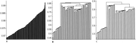
A: Dendrogram tree for the original fMRI data set. B: Dendrogram after the first pass of the sharpening algorithm. C: Dendrogram for the twice‐sharpened data. Notice, how with each filtering step the chaining effect diminishes and the structure of the data becomes more evident.
Table III.
Comparative table of the number of voxels retained before and after dendrogram sharpening for different parameters
| nfluff (1st DSH) | nfluff (2nd DSH) | ncore | No. of voxels prior DSH | No. of voxels after 1st DSH | No. of voxels after 2nd DSH |
|---|---|---|---|---|---|
| 1 | 10 | 20 | 1,455 | 183 | 59 |
| 2 | 10 | 20 | 1,455 | 141 | 59 |
| 2 | 10 | 30 | 1,455 | 157 | 75 |
| 1 | 10 | 40 | 1,455 | 201 | 96 |
| 2 | 10 | 40 | 1,455 | 167 | 94 |
| 2 | 10 | 50 | 1,455 | 176 | 107 |
| 2 | 10 | 70 | 1,455 | 179 | 110 |
First three columns list the sharpening parameters (ncore, nfluff) applied to the data set. The remaining columns list the number of voxels before and after dendrogram sharpening (DSH).
Data Reduction
Paradigm 1
From the total number of voxels in the four slices, the majority of voxels with a SNR in the first decile were discarded leaving about 4,000 voxel time courses for future analysis. For each voxel, the correlation coefficient was computed with all other voxels and a frequency index determined to count the number of significant correlations (correlation coefficient >0.5). About 1,000 voxels were found that had more than four significant correlations with other voxels. After the first sharpening, the number of voxels reduced to 90, and the second sharpening eliminated an additional 20 voxels.
Paradigm 2
After discarding the voxels with SNR in the first decile from the total number of observations in 20 slices with 64 × 64 voxels, the number of voxels was reduced to about 10,000. Setting the correlation threshold to 0.5 and, as before, requiring at least five significant correlations for each voxel, reduced the data set to about 1,200 voxels.
The first sharpening with nfluff = 2 and ncore = 40 resulted in about 320 voxels and was reduced further to 130 voxels after the second pass with sharpening with parameters nfluff = 10 and ncore = 40.
It is worth noting that application of the initial preprocessing steps, which include motion and trend removal, significantly altered the distribution of the cross correlation coefficients. The shape of the distribution for the preprocessed data appears to be more symmetrical than the positively skewed form of the raw data distribution (see solid and dotted lines on Fig. 10, respectively).
Figure 10.
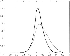
Distribution of the cross‐correlation coefficients for the raw (dotted) and preprocessed (solid) data set. Motion and trend removal significantly impact the shape of the distribution making it more symmetrical.
RESULTS AND DISCUSSION
Obtained results are consistent across all four subjects participating in the study. For each of the four subjects activations specific to the motor task paradigms were detected. To avoid redundancy, we present only the results from two different subjects.
Paradigm 1
After the first pass of the algorithm over the data, two clusters containing 51 and 20 voxels, respectively (Fig. 11A,B), were identified. Active voxels in cluster A could be attributed to motion and vascular artifacts. Voxels constituting cluster B suggest the presence of the activation in SMA and primary motor cortex. The application of the second sharpening produced three clusters (Fig. 11(C–E)). Cluster E is absolutely identical to cluster B. However, artifacts previously combined in cluster A are separated now into two different clusters C and D, each containing 20 and 17 voxels, respectively. The classification of the remaining voxels (C → F, D → G, E → H) confirms our initial hypothesis clearly indicating strong activation in the sensorimotor cortex, SMA, premotor cortex, and precentral gyrus for cluster H, blood vessels (superior sagittal sinus) for cluster F, and motion related artifacts in cluster G.
Figure 11.
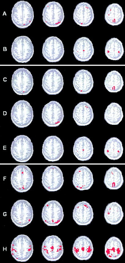
Paradigm 1. A, B: Cluster identified in the once‐sharpened data. C–E: Clusters identified in the twice‐sharpened data. F–H: Clusters C, D, and E after the final classification of the voxels discarded during sharpening. Clusters F and G represent vascular and motion artifacts. Cluster H represents primary motor cortex and SMA.
Even though the paradigm frequency 0.1 Hz contributes to each of the mean time courses of resulting clusters F, G, H (Fig. 12), it is dominant only for the cluster H associated with motor activation. The major contribution to cluster G comes from frequencies <0.01 Hz. This occurs at the location where the spatial gradient is large and is possibly related to the low‐frequency motion artifact. Also, respiratory (0.2–0.4 Hz) and cardiac bands (∼1.2 Hz) are best observed in the spectra of cluster F.
Figure 12.
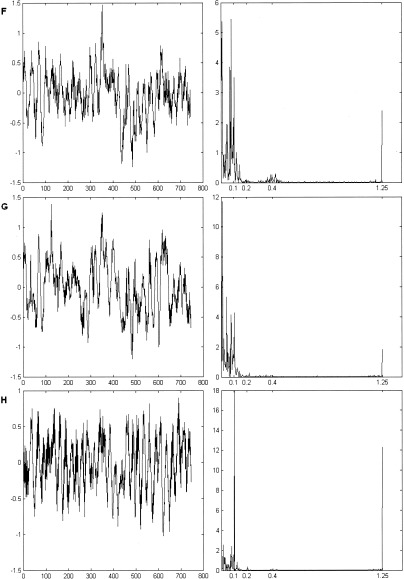
Paradigm 1. Mean time courses and corresponding Fourier spectra for the identified clusters. The paradigm frequency (0.1 Hz) significantly contributes to all three average time courses and is dominant for the cluster H.
Hierarchical clustering combined with dendrogram sharpening proved to be robust to the artifacts, such as motion and trend. Even when applied directly to the raw data (prior motion and trend removal), DSH identifies activation in motor cortex regions and separates vascular artifacts producing clusters similar to the cluster F and H (Figs. 11, 12). Voxels constituting cluster G do not pass the required correlation threshold and are excluded from the cluster analysis.
Paradigm 2
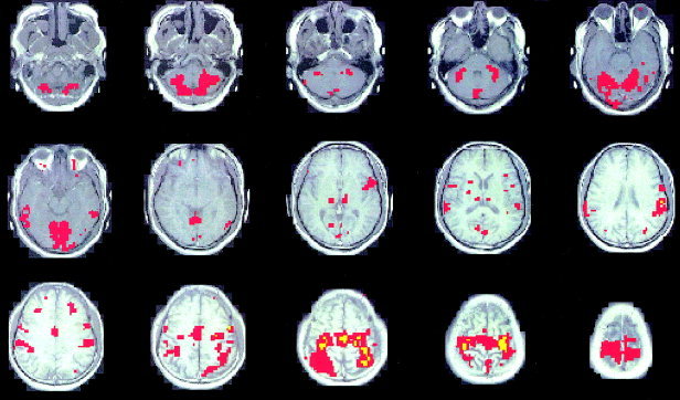
Using the method of inconsistent edges, four clusters, containing 20, 11, 14, and 30 voxels respectively, were identified in the twice sharpened data. After the classification, the majority of discarded voxels (about 1,000) were reassigned to cluster A (Fig. 13). The other three clusters (B, C, D) are shown in Figure 14. Cluster A shows strong activation in the primary sensorimotor cortex, SMA, cerebellum and parietal lobule, Broadmann's areas 7 and 40, known to have contralateral connections with primary somatosensory cortex, The particular activation in the parietal cortex is related to our subject who is an experienced hockey player.
Figure 13.
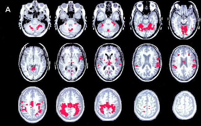
Paradigm 2. The first cluster (A), identified in the twice‐sharpened data after the final classification of the discarded voxels, shows activation in the motor cortex and related areas.
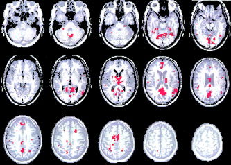
Figure 14.
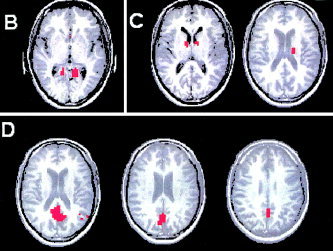
Paradigm 2. The remaining three clusters (B–D) identified in the twice‐sharpened data after the final classification of the discarded voxels.
Clusters B and C were specific to the retrosplenial area (Fig. 14B) and thalamus (Fig. 14C), respectively. The vascular flow artifacts were separated into the fourth cluster (Fig. 14D). For the sake of space, only slices containing the active voxels are presented for the last three clusters. The mean time course and the corresponding power spectrum for each of the four clusters are shown in Figure 15. All time series exhibit a hemodynamic delay of about 6 sec relative to the stimulus onset. In addition, the dominant frequency peak occurs at the paradigm frequency (0.016 Hz). Otherwise, the structure of the Fourier spectra is very diverse. Out of the four identified clusters, cluster A has the least Fourier components.
Figure 15.
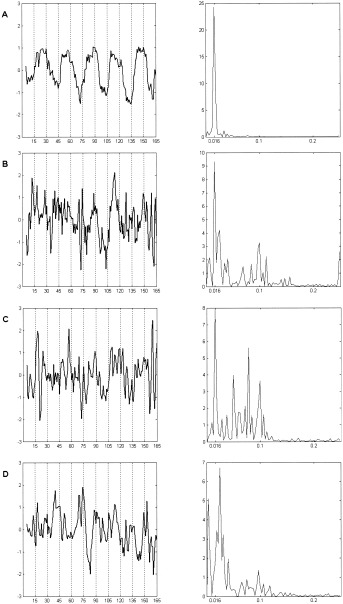
Paradigm 2. Spectral analysis of the average time courses corresponding to the four identified clusters. Notice the presence of the paradigm associated frequency of 0.016 Hz in all four spectra as well as the large range of the contributing frequencies for clusters B, C, and D.
To evaluate the performance of the sharpening algorithm, results were compared to those obtained using a conventional statistical approach (SPM) by using a convolved boxcar function matching the expected hemodynamic response (single‐voxel P = 0.00001). Even though cluster analysis is fundamentally different from the SPM, the latter was chosen as a standard procedure to gain more confidence in the resulting maps.
The SPM map for the first 5 sec on/off paradigm is omitted since the maps detected by the two different methods are virtually the same. Figure 16 shows two graphs, corresponding to the average time course of cluster H (Fig. 11) resulting from the sharpening algorithm and of the SPM activation pattern, respectively. For the convenience of the readers, only the first 100 time points are plotted to show increased detail. The correlation coefficient between the two mean time courses, resulting from the application of clustering and SPM, is equal to 0.91 suggesting almost identical results. The high frequency artifact seen here is related to the unaliased cardiac rate since the TR was very short (400 msec).
Figure 16.
Paradigm 1.The mean time courses of the motor‐activation–related cluster identified using dendrogram sharpening (solid line) and SPM map (dashed line). The high frequency is attributed to the cardiac rate.
Areas of activation associated with the second paradigm (30 sec on/off finger‐tapping) detected by SPM also appear to be very similar to the clustering results (compare Figs. 13A and 17). The value of the correlation coefficient between the mean time courses in this case is 0.99. High similarity between the two methods was observed for all four subjects and both paradigms used in the experiment (Table IV).
Figure 17.
Paradigm 2. SPM analysis of voxels in the sensorimotor cortex and cerebellum (compare to Fig. 13).
Table IV.
Number of clusters identified in each of the data sets attributed to the particular subject and paradigm
| Subject 1 | Subject 2 | Subject 3 | Subject 4 | |
|---|---|---|---|---|
| Paradigm 1 | ||||
| No. of clusters | 3 | 3 | 2 | 3 |
| corr. coef | 0.91 | 0.91 | 0.93 | 0.90 |
| Paradigm 2 | ||||
| No. of clusters | 4 | 5 | 4 | 3 |
| corr. coef | 0.99 | 0.98 | 0.99 | 0.99 |
The correlation coefficient shows the degree of similarity between the mean time courses of the motor‐activition‐related cluster and SPM map.
We compared our algorithm with another clustering technique known as fuzzy C‐means. The major drawback of the basic K‐ and fuzzy C‐means algorithm is the requirement to specify the expected number of clusters; however, the attractive part of both algorithms is their high computational efficiency. We illustrate the result of the fuzzy C‐means analysis for the second 30‐sec on/off paradigm. The number of clusters was chosen to be four, which is exactly the number of groups identified by the sharpening method. One of the produced clusters showed motor activations identical to those in Figure 13A. The correlation coefficient between the mean time courses of the two clusters resulting from our method and fuzzy C‐means was 0.99. We, therefore, omitted the corresponding image. The second largest cluster is presented in Figure 18 and encompasses some features contained in clusters B, C, and D in Figure 14 in addition to some vascular effects. The remaining two clusters contained only 3–4 voxels and were, therefore, meaningless and are not shown. Both clustering methods proved to be capable of identifying activations in the motor areas and produced almost identical results. Hierarchical clustering combined with dendrogram sharpening was more selective in separating certain features into different clusters. Fuzzy C‐means splits all the voxels into two different groups: one with pronounced on/off pattern of the paradigm and the other containing all the remaining voxel time courses. The main advantage of the dendrogram sharpening in hierarchical clustering is that it does not require any prior knowledge of the number of clusters or their locations. Sharpening and final classification algorithms are both very simple and easy to implement. The recursive calls used in the sharpening procedure make it simple to program. However, they demand quite a bit of CPU time and, especially, system memory. We used a 1.7GHz Pentium IV computer with 1.5GB RAM and were able to process a whole data set in less than an hour.
Figure 18.
Second largest of four clusters resulting from fuzzy C‐means algorithm (paradigm 2). It contains some features seen in clusters B–D and also vascular artifacts.
Sharpening proved to be a fruitful method when the activation is strong as for primary cortex stimulations, though it requires more rigorous theoretical studies and further modifications. The only limitation of this algorithm is the proper specification of the two required sharpening parameters. However, the choice of these values is defined by the size and the structure of the data set. It was mentioned earlier that the value of the nfluff and ncore parameters would impact the number of resulting voxels (Table III). In fact, all of the listed values would produce very similar clustering results, since the final classification algorithm assigns the voxels set aside during sharpening to the identified cores. For example, choosing the combination of parameters that leaves more voxels for clustering, would allow a researcher to get an idea of the expected activation pattern prior to the classification. High values of ncore will also shorten the time of sharpening.
The recommendations on the choice of the settings for the classification algorithm are somewhat different. The latter method, as it was introduced by McKinney [ 1995], would partition the entire set into n clusters. Our original fMRI data is contaminated by physiological noise, subject motion, and scanner artifacts. We propose to classify not all the objects but only those located within a certain radius. Since the distance measure is a function of the correlation coefficient, only those voxels that are highly correlated with the identified centers will be reassigned. For this purpose, the value of the classification threshold is defined. Recall that the classification algorithm works from the bottom to the top of the tree and initially every data point represents a cluster. Two clusters linked together in the original dendrogram will be classified if the distance between them is less than the value of the classification threshold. Remember that the single linkage tree, due to the lack of spatial separation in the data, exhibits strong chaining behavior and, thus, many top nodes tend to have a very small child. These small children often represent the outliers in the data connected to the high‐density regions at the last stage of linking. The higher the threshold value, the more voxels will be classified. Figure 19 illustrates the dependence of the correlation coefficient between the mean time courses of the motor‐activation cluster and SPM activation map on the value of the classification threshold. As one can see, at first the results of the algorithms are getting closer as the correlation coefficient approaches its maximum for the threshold value of 0.8, but then the classification results worsen as more and more voxels have been reassigned to the cluster groups. The declination is due to the reassignment of “noisy” voxels that have low correlation coefficients. Though the correlation coefficient remains high when all the voxels are reassigned, the optimal choice of the classification threshold for this particular data set would be 0.8. The latter value depends on the maximum distance between the linked objects in the original dendrogram and varies for different data sets and preprocessing settings. In our analyses, the classification threshold is set to 0.8*agglomeration value of the root node. This threshold consistently yielded good results in all data sets.
Figure 19.
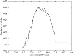
The correlation coefficient between the mean time courses of the SPM activation map and motor activation cluster resulting from our method as a function of the classification threshold.
CONCLUSIONS
The present study demonstrates that dendrogram sharpening might be a very helpful tool for analysis of activation patterns in fMRI. This approach is model free and does not require prior assumption about the number and location of the clusters. The single linkage method, used to group the data, is preferable over the complete or average linkage algorithms, because of its ability to reveal the modal regions of the data. The large amount of fMRI data makes it difficult to detect networks of brain activity. Sharpening significantly simplifies the identification by reducing the data set and preserving its structure. Though dendrogram sharpening is sensitive to its parameters, it is possible to identify appropriate values to yield a meaningful result.
Acknowledgements
This work was partially supported by a grant from the Royalty Research Fund and the National Institute of Child Health and Human Development (HD33812). We also thank George Barrett, Ph.D. (University of Washington) for reviewing the manuscript.
REFERENCES
- Baumgartner R, Windischberger C, Moser E (1998): Quantification in functional magnetic resonance imaging: fuzzy clustering vs. correlation analysis. MRI 16: 2: 115–125. [DOI] [PubMed] [Google Scholar]
- Baumgartner R, Ryner L, Richter W, Summers R, Jarmasz M, Somorjai R (2000a): Comparison of two exploratory data analysis methods for fMRI: fuzzy clustering vs. principal component analysis. MRI 18: 89–94. [DOI] [PubMed] [Google Scholar]
- Baumgartner R, Somorjai R, Summers R, Richter W, Ryner L (2000b): Novelty indices: identifiers of potentially interesting time‐courses in functional MRI data. MRI 18: 845–850. [DOI] [PubMed] [Google Scholar]
- Cordes D, Haughton V, Carew J, Arfanakis K, Maravilla K (2002): Hierarchical clustering to measure connectivity in fMRI resting‐state data. MRI 20: 305–317. [DOI] [PubMed] [Google Scholar]
- Filzmoser P, Baumgartner R, Moser E (1999): A hierarchical clustering method for analyzing functional MR images. MRI 17: 817–816. [DOI] [PubMed] [Google Scholar]
- Goutte C, Toft P Rostrup E, Nielsen FA, Hansen LK (1999): On clustering fMRI time series. Neuroimage 9: 298–310. [DOI] [PubMed] [Google Scholar]
- Hartigan JA (1975): Clustering algorithm. New York: John Wiley & Sons. [Google Scholar]
- Hartigan JA (1977a): Asymptotic distributions for clustering criteria. Ann Stat. [Google Scholar]
- Hartigan JA (1977b): Distribution problems in clustering In: Van Ryzin J, ed. Classification and clustering. New York: Academic Press; p 45–72. [Google Scholar]
- Hartigan JA (1981): Consistency of single linkage for high‐density clusters. Am Stat 76: 388–392. [Google Scholar]
- Jain AK, Dubes RC (1988): Algorithms for clustering data. Englewood Cliffs, NJ: Prentice‐Hall. [Google Scholar]
- McKeown MJ, Sejnowski TJ (1998): Independent component analysis of fMRI data: examining the assumptions. Hum Brain Mapp 6: 368–372. [DOI] [PMC free article] [PubMed] [Google Scholar]
- McKinney S (1995): Autopaint: A Toolkit for visualizing data in four or more dimensions. PhD thesis, University of Washington, Seattle.
- Sychra JJ, Bandettini PA, Bhattacharya N, Lin Q (1994): Synthetic images by subspace transforms. I. Principal components images and related filters. Med Phys 21: 193–201. [DOI] [PubMed] [Google Scholar]
- Tanbe J, Miller D, Tregellas J, Freedman R, Meyers F (2002): Comparison of detrending methods for optimal fMRI preprocessing. Neuroimage 15: 902–907. [DOI] [PubMed] [Google Scholar]
- Tukey JW (1977): Exploratory data analysis. Reading, MA: Addison‐Wesley Publishing Co. [Google Scholar]
- Tukey PA, Tukey JW (1981): Data‐driven view selection. Agglomeration and sharpening In: Barnett V, ed. Interpreting multivariate data. New York: John Wiley and Sons; p 215–243. [Google Scholar]
- Windischberger C, Barth M, Lamm C, Schroeder L, Bauer H, Gur R, Moser E (2002): Fuzzy cluster analysis of high‐field functional fMRI data. Artificial Intelligence in Medicine 675: 1–21. [DOI] [PubMed] [Google Scholar]