Analysis and visualization of single‐trial event‐related potentials

Abstract

In this study, a linear decomposition technique, independent component analysis (ICA), is applied to single‐trial multichannel EEG data from event‐related potential (ERP) experiments. Spatial filters derived by ICA blindly separate the input data into a sum of temporally independent and spatially fixed components arising from distinct or overlapping brain or extra‐brain sources. Both the data and their decomposition are displayed using a new visualization tool, the “ERP image,” that can clearly characterize single‐trial variations in the amplitudes and latencies of evoked responses, particularly when sorted by a relevant behavioral or physiological variable. These tools were used to analyze data from a visual selective attention experiment on 28 control subjects plus 22 neurological patients whose EEG records were heavily contaminated with blink and other eye‐movement artifacts. Results show that ICA can separate artifactual, stimulus‐locked, response‐locked, and non‐event‐related background EEG activities into separate components, a taxonomy not obtained from conventional signal averaging approaches. This method allows: (1) removal of pervasive artifacts of all types from single‐trial EEG records, (2) identification and segregation of stimulus‐ and response‐locked EEG components, (3) examination of differences in single‐trial responses, and (4) separation of temporally distinct but spatially overlapping EEG oscillatory activities with distinct relationships to task events. The proposed methods also allow the interaction between ERPs and the ongoing EEG to be investigated directly. We studied the between‐subject component stability of ICA decomposition of single‐trial EEG epochs by clustering components with similar scalp maps and activation power spectra. Components accounting for blinks, eye movements, temporal muscle activity, event‐related potentials, and event‐modulated alpha activities were largely replicated across subjects. Applying ICA and ERP image visualization to the analysis of sets of single trials from event‐related EEG (or MEG) experiments can increase the information available from ERP (or ERF) data. Hum. Brain Mapping 14:166–185, 2001. © 2001 Wiley‐Liss, Inc.

INTRODUCTION

Single‐trial event‐related potential (ERP) data are usually averaged prior to analysis to increase their signal/noise relative to non‐time and ‐phase‐locked electroencephalographic (EEG) activity and non‐neural artifacts. However, response averaging ignores the fact that the response may vary widely across trials in amplitude, time course, and scalp distribution. This temporal and spatial variability is hidden by response averaging, but may in fact reflect changes in subject performance or in subject state possibly linked to fluctuations in expectation, attention, arousal, task strategy, or other factors [Haig et al., 1995; Yabe et al., 1993]. Thus, conventional averaging methods may not be suitable for investigating brain dynamics arising from unpredictable changes in subject state and/or from complex interactions between subject state and experimental events.

Analysis of single event‐related trial epochs may potentially reveal more information about event‐related brain dynamics than simple response averaging, but faces three signal processing challenges: (1) difficulties in identifying and removing artifacts associated with blinks, eye‐movements and muscle noise, which are a serious problem for EEG interpretation and analysis, especially when blinks and muscle movements occur quite frequently as with some patient groups; (2) poor signal‐to‐noise ratio arising from the fact that non‐phase‐locked background EEG activities typically are much larger than phase‐locked response activity, making extraction of event‐related brain dynamics difficult; (3) trial‐to‐trial variability in latencies and amplitudes of both event‐related response features and endogenous EEG measures. In large part, these problems are hidden rather than solved by response averaging.

EEG artifacts

Contamination of EEG activity by eye movements, blinks, and muscle artifacts seriously interfere with the interpretation and analysis of ERPs. A common strategy is to average trials time‐locked to all similar experimental events and discard or ignore averages of data from frontal and temporal electrodes. Often, EEG segments with artifacts larger than an arbitrarily preset value are rejected. However, when limited data are available, or blinks and muscle movements occur too frequently as with some patient groups, the amount of data lost to artifact rejection may be unacceptable. For example, Small [1971] reported a visual ERP experiment conducted on autistic children who produced EOG artifacts in nearly 100% of the trials. Under these conditions, differences in background EEG make averaged ERPs of the few artifact‐free trials too unstable to allow useful analysis.

Other methods attempt to regress out eye movement artifacts based on reference signals collected near the eyes [Hillyard and Galambos, 1970; Verleger et al., 1982; Whitton et al., 1978; Woestenburg et al., 1983a]. However, these methods also eliminate recorded activity common to the reference channel and neighboring electrodes, and may also spread neural activity unique to the reference channel into other sites. Better methods are needed for removing artifacts that preserve all of the EEG data prior to averaging or single‐trial analysis.

Spontaneous EEG

ERPs, particularly those evoked by visual stimuli, often contain prominent remnants of rhythmic EEG activity, particularly at alpha frequencies, although non‐visual, non‐alpha oscillatory ERP activity may also occur [Makeig and Galambos, 1982]. In some subjects, large amounts of residual alpha activity may make accurate assessment of standard ERP peak measures impossible. This so‐called ERP “alpha ringing” may represent stimulus‐induced phase resetting of ongoing alpha activity [Brandt, 1997; Kolev and Yordanova, 1997] from multiple alpha processes [Florian et el., 1998], and may differentially affect the amplitudes of both early [Brandt et al., 1991] and late [Haig and Gordon, 1998] ERP components. Interactions between pre‐stimulus theta activity and late ERP components have also been noted [Polich, 1997; Yordanova and Kolev, 1997]. Improved separation of artifacts, background EEG processes, and single‐trial ERP components could allow more accurate ERP measurements, as well as more detailed study of interactions between evoked response features and ongoing EEG activity.

Response variability

The late positive complex (LPC), also called the P300 or P3, in responses to anticipated but unpredictable stimuli typically peaks more than 300 ms after target onset. However, LPC peak amplitudes, latencies, and wave shape may vary widely from trial to trial [Kutas et al., 1977]. Several studies have reported a number of different single‐trial response subtypes [Haig et al., 1995; Suwazono et al., 1994]. Classifying subtypes of single‐trial scalp ERPs may allow investigating brain dynamics involving transitory or intermittent subject cognitive states, but is difficult because the presence of large artifacts and non‐task‐related background EEG activity in single trials.

New approaches

We introduce here an approach to analyzing and visualizing multichannel single‐trial unaveraged ERP records that alleviates these problems. First, we describe a new visualization tool, the “ERP image,” an effective method for visualizing phase, amplitude, and timing relations between event‐related EEG activity time‐locked to experimental events (e.g., stimulus onsets and/or subject responses) in sets of single trials. We then demonstrate the benefits of decomposing sets of multichannel single‐trial ERP epochs using blind source separation [Jutten and Herault, 1991]. In this study, we apply independent component analysis (ICA) [Comon, 1994] using the infomax approach of Bell and Sejnowski [1995], Amari et al. [1996], and Lee et al. [1999] to carry out blind source separation. Infomax ICA is one of a family of algorithms [Cardoso and Laheld, 1996; Comon, 1994; Jutten and Herault, 1991] that exploit independence to perform blind source separation. ICA algorithms can separate complex multichannel data into spatially fixed and temporally independent components whose linear mixtures form the input data records, without detailed models of either the dynamics or the spatial structure of the separated components.

These analytical tools were applied to 50 sets of single‐trial EEG epochs collected from 28 normal controls and 22 neurologic patients. In this paper, we demonstrate, through three data sets, the power of these new analysis and visualization methods for increasing the information about event‐related brain dynamics that can be derived from both “clean” or “noisy” EEG data. Improvements in analyzing data heavily contaminated by movement artifacts may be important in clinical and developmental EEG studies. Our approach may also increase the range of usable paradigms for studies of normal adult brain processing. When ICA was applied to single‐trial target‐response epochs, the derived components were time‐locked to stimulus onsets and/or subject responses in distinctly different ways. We also propose an effective method for deriving optimized ERP averages with minimal temporal smearing from performance fluctuations.

METHODS AND MATERIALS

Subjects

Data were collected from 28 normal controls, and ten high‐functioning autistic and 12 brain lesion subjects. All subjects had normal or corrected‐to‐normal vision. The control subjects had no history of substance abuse, special education, major medical or psychiatric illness, or developmental or neurological disorder. The autistic subjects met DSM‐III‐R [American Psychiatric Association, 1987] criteria for autistic disorder, as well as criteria from the Autism Diagnostic Interview, the Autism Diagnostic Observation Schedule [Lord et al., 1994], and the Childhood Autism Rating Scale [Schopler et al., 1980]. Lesion sites in the patients were verified by neuroradiological examination of magnetic resonance images. The stroke and autistic subjects had no additional neurological or psychiatric diagnoses.

EEG data collection

EEG data were recorded from 31 scalp electrodes, 29 placed at locations based on a modified International 10‐20 system, one placed below the right eye (VEOG), and one placed at the left outer canthus (HEOG). All 31 channels were referred to the right mastoid and were digitally sampled for analysis at 256 Hz with a 0.01‐ to 100‐Hz analog bandpass plus a 50‐Hz low‐pass filter. Subjects participated in a 2‐hour visual spatial selective attention task in which they were instructed to attend to filled circles flashed in random order in five locations laterally arrayed 0.8 cm above a central fixation point. Locations were outlined by five evenly spaced 1.6‐cm blue squares displayed on a black background at visual angles of 0°, ± 2.7°, and ± 5.5° from fixation. An attended location was marked by a green square throughout each 72‐sec experimental block. Subjects were instructed to maintain fixation on the central cross and press a button as quickly as possible each time they saw a filled circle appear in the attended location. The location of the attended square was counterbalanced across experimental blocks [for further details see Makeig et al., 1999a; Townsend and Courchesne, 1994]. Prior to analysis, those trials wherein the subject blinked or moved the eyes at the moment of presentation of the visual stimulus were rejected because stimulus perception might have been impaired.

A visualization tool, the ERP image

The “ERP image” is a new method for visualizing variability in the latencies and amplitudes of event‐related responses [Jung et al., 1999, 2000b, 2001]. To form an ERP image, potentials recorded at one scalp channel in each trial (or the time courses of activations of one response component) are sorted in order of a relevant response measure (e.g., subject response time) and then plotted as parallel colored lines forming a colored rectangular image. The ERP image may be displayed before or after smoothing with a narrow (e.g., 2‐30 trial) moving window to increase the salience of time‐ and/or phase‐locked response features.

Independent component analysis

Independent component analysis [Comon, 1994] is a method for solving the blind source separation problem [Jutten and Herault, 1991]: to recover N‐independent source signals, s = {s ₁(t),…,s _N(t)} (e.g., different voices, music, or other sound sources) from N linear mixtures, x = {x ₁(t),…,x _N(t)}, modeled as the result of multiplying the matrix of source activity waveforms, s, by an unknown square matrix A (i.e., x = As). Given minimal a priori knowledge of the nature of the sources or of the mixing process, the task is to recover a version, u, of the original sources, identical to s, save for scaling and source order. To do this, it is necessary to find a square matrix, W, specifying filters that linearly invert the mixing process (i.e., u = Wx). The key assumption used to distinguish sources from mixtures is that sources, s_i, are statistically independent, though their mixtures, x_i, are not. In contrast with decorrelation techniques such as PCA, which ensure only that output pairs are uncorrelated (< u_i u_j> = 0, ∀ ij), ICA approaches a much stronger criterion, statistical independence, which occurs when the multivariate probability density function (p.d.f.), f(u), factorizes, e.g.,

Strict statistical independence requires that all second‐order and higher‐order correlations of the u_i are zero, whereas decorrelation only seeks to minimize second‐order statistics (covariance or correlation).

Bell and Sejnowski [1995] proposed a simple neural network “infomax” algorithm that blindly separates mixtures, x, of independent sources, s, using information maximization (infomax). They showed that maximizing the joint entropy, H(y), of the output of a neural processor minimizes the mutual information among the output components, y_I = g(u_i), where g(u_i) is an invertible bounded nonlinearity and u = Wx. Recently, Lee et al. [1999] extended the ability of the infomax algorithm to perform blind source separation on linear mixtures of sources having either sub‐ or super‐Gaussian distributions. For further details, see these sources and Jung et al. [2000a, 2000b]. Here, we apply the infomax algorithm to collections of 31‐channel single‐trial EEG records from a visual selective‐attention experiment.

Applying ICA to single‐trial EEG epochs

Use of ICA for blind source separation of EEG data is based on two plausible premises: (1) EEG data recorded at multiple scalp sensors are linear sums of temporally independent components arising from spatially fixed brain networks or extra‐brain sources; (2) the spatial spread of electric current from sources by volume conduction does not involve significant time delays. For further details regarding ICA assumptions underlying EEG analysis, see Makeig et al. [1997, 1999a], Jung et al. [1998a] (see Fig. 1)

Figure 1.

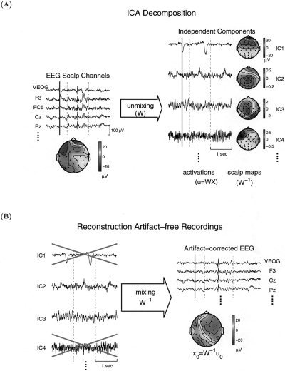
Schematic overview of ICA applied to EEG data. (A) A matrix of single‐trial EEG data, x, recorded at multiple scalp sites (only four are shown), are used to train an “unmixing” weight matrix, W, to minimize the statistical dependence of the equal number of outputs, u = Wx (four shown here). After training, ICA components consist of time series (the rows of u) giving the time courses of activation of each component, plus fixed scalp topographies (the columns of W⁻¹) giving the projections of each component onto the scalp sensors. (B) Some ICA components account exclusively or predominantly for artifactual activity, for example component IC1, generated by blinks, or IC4, generated by temporal muscle activity. Others account for various evoked and/or spontaneous EEG activity (e.g., IC2, IC3). Artifact‐free EEG signals, x₀, can be obtained by mixing and projecting back onto the scalp channels selected non‐artifactual ICA components (IC2 + IC3) by multiplying the selected activation waveforms, u₀, by the inverse mixing matrix, W ⁻¹ [Adapted from Jung et al., 2000b].

Several previous applications of ICA to electrophysiological data have focused on event‐related response averages [Jung et al., 1998a; Makeig et al., 1996, 1997, 1999a, 1999b]. Applying ICA to spontaneous or event‐related single‐trial EEG epochs is more promising but has been less explored [Jung et al., 1999, 2000b, 2001; Makeig et al., 1996, 2000a, 2000b, 2000c; McKeown et al., 1998]. In single‐trial EEG analysis, the rows of the input matrix, x, are EEG signals recorded at different electrodes, and the columns are measurements recorded at different time points (Fig. 1A, left). ICA finds an “unmixing” matrix, W, which decomposes or linearly unmixes the multichannel scalp data into a sum of maximally temporally independent and spatially fixed components, u = Wx. The rows of the output data matrix, u, are time courses of activation of the ICA components. The columns of the inverse matrix, W ⁻¹, give the relative projection strengths of the respective components at each of the scalp sensors (Fig. 1A, right). These scalp weights give the scalp topography of each component, and provide evidence for the components' physiological origins (e.g., eye activity projects mainly to frontal sites, etc.). All scalp maps shown here were computed using the original right‐mastoid reference. Event‐related brain signals accounted for by single‐ or multicomponents can be obtained with true polarity and μV amplitudes by projecting selected ICA components back onto the scalp, x₀ = W⁻¹ u₀, where u₀ is the matrix, u, of activation waveforms with rows representing activations of irrelevant component activations set to zero (Fig. 1B).

Component clustering

To study the cross‐subject stability of independent components derived by infomax ICA applied to single‐trial epochs, a symmetrical Mahalanobis distance measure (see Appendix), calculated from a combination of scalp maps and power spectra of the component activations was used to cluster the set of components obtained from multiple subjects. Individual component clusters were characterized by their mean cluster map and activity spectrum.

Numerical methods

Extended‐ICA decomposition was performed on 31‐channel, 1‐sec data epochs from 300 to 700 target stimulus trials for each of 28 normal control and 22 clinical subjects using routines coded in MATLAB 5 and C running on a Pentium II 400 MHz PC with 512 MB RAM. Only target trials in which the subject pressed the response button within the allowed (150–1000 msec) time window were analyzed. The learning batch size was 50. The initial learning rate, 0.004, was gradually reduced to 10⁻⁷ during training, which required 2–6 hours per subject to converge in MATLAB (or less than one‐half hour using optimized C‐language binary code). Our previous results [Jung et al., 2000a; Makeig et al., 1996, 1997, 1998, 1999a] as well as the results we report here have shown that ICA decomposition is relatively insensitive to the exact choice or learning rate or batch size. A MATLAB toolbox for performing the analyses and visualizing the results, plus binary code for speeding the decomposition is available for download at http://www.cnl.salk.edu/~scott/ica.html.

Characterizing independent components

For each set of 31‐channel single‐trial target responses, ICA derived 31 maximally independent components having temporally distinct activities arising from different brain or extra‐brain sources.

Eye blink components

Blink‐related component(s) were identified by the following procedure. (1) All 31‐channel ICA activations were displayed and searched for the component(s) with time courses resembling blink activity (brief, large amplitude changes). (2) The scalp topographies of the candidate components were plotted to provide further evidence of their physiological origin (eye activity projects most strongly to periocular and far frontal sites). (3) When necessary, source localization was performed to find effective dipoles for the component(s) using BESA [Scherg, 1990] to judge whether these were located in or near the eyes.

Eye movement components

Component(s) accounting for lateral eye movements time locked to visual stimulus presentations were identified by the following. (1) Separately averaging the single‐trial EEG records time‐locked to target stimuli presented at five different locations. (2) Applying the spatial filters derived by ICA from all the EEG trials to the resulting five 31‐channel ERPs and searching for components whose time courses differed systematically with stimulus location. Our assumption here was that involuntary saccadic movements following stimulus presentations would systematically change in both amplitude and direction as a function of the distance and direction from the fixation point to target location. There should be a systematic relationship for components accounting for saccadic eye movements, but not for other components accounting for other brain (or extra‐brain) activities. (3) Verifying the nature of the candidate eye‐movement components by plotting their scalp topographies. The components accounting for lateral eye movements projected most strongly to far frontal sites, and showed a polarity difference between the two periocular sites.

ERP images were used to identify the nature of neural activity accounted by other component. One‐second single‐trial activations of each component were aligned to stimulus onsets and to the subject's responses to help us determine if the EEG activity accounted for by the component was stimulus‐locked, response‐locked, or non‐phase‐locked (see Results).

RESULTS

ERP images

ERP images can be used to visualize variability in the amplitudes and latencies of event‐evoked responses, either by visualizing single‐channel EEG epochs themselves, or by visualizing the single‐trial activations of components of the data. An example, shown in Figure 2 (left), plots 645 single‐trial ERP epochs recorded at the central parietal site Pz from a control subject and time‐locked to onsets of target stimuli (left vertical line). Each colored horizontal trace represents a 1‐s single‐trial ERP record whose potential variations are color‐coded (see color bar at right). The jagged black vertical line shows the subject's response latency in each trial. Note the trial‐to‐trial fluctuations in both ERP latency and reaction time. The average of these trials and the median response time (RT) are plotted below the ERP image. Next, the same single trials were sorted in order of increasing subject RT and plotted both before (middle) and after (right) smoothing with a 20‐trial rectangular moving average.

Figure 2.

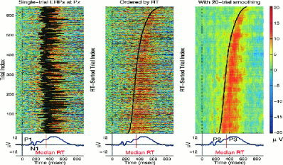
ERP images of single‐trial target response data from a visual selective attention experiment. (Left) Single‐trial ERPs recorded at a parietal electrode (Pz) from the control subject and time‐locked to onsets of visual target stimuli (left thin vertical line) with superimposed subject response times (RT) (thick black line). (Middle) The same 645 single trials, sorted (bottom to top) in order of increasing RT. (Right) The same sorted trials smoothed with a 20‐trial moving window advanced through the data in one‐trial steps to increase response signal‐to‐noise ratio and minimize the influence of EEG activity not consistently time‐ and phase‐locked to experimental events. The average of all 645 trials, shown below each ERP image, contains characteristic peaks (including the indicated P1, N1, P2, and P3 peaks) whose systematic relationships to behavioral RT are most clearly visualized in the right and central images.

Note (Fig. 2, right) that in nearly all trials the early features (P1, N1) are time‐locked to stimulus onset (i.e., they are stimulus‐locked), whereas the later positive “P3” feature follows the response in all but the longest‐RT trials (i.e., it is mainly response‐locked), a fact not evident in the ERP trial average (bottom).

An ERP image allows direct visualization of single event‐related EEG trials and their contributions to the averaged ERP. An ERP image also makes visible relationships between subject behavior and amplitudes/latencies of individual event‐related responses, and reveals several problems with conventional response averaging. First, few if any trials in these data had a time course that closely resembled the averaged ERP waveform (i.e., the bottom traces). Second, later ERP components systematically time‐locked to subject responses were temporally smeared in the stimulus‐locked average, making the averaged ERP an imprecise representative of the underlying event‐related response processes. Third, the temporal relationship between the time‐varying events, such as RT and the “P3” peak were confused in the ERP average. For this subject, the average response (shown in the bottom traces) gives the impression that the onset of the positive (red) “P3” preceded the median RT (vertical lines crossing the ERP traces) by about 80 ms, whereas the ERP images (top) clearly show that, in single trials, the “P3” onset actually systematically followed RT.

The ERP image can be used to display single‐trial raw data and their independent component activations and to characterize the nature of independent components (see Fig. 5).

Figure 5.

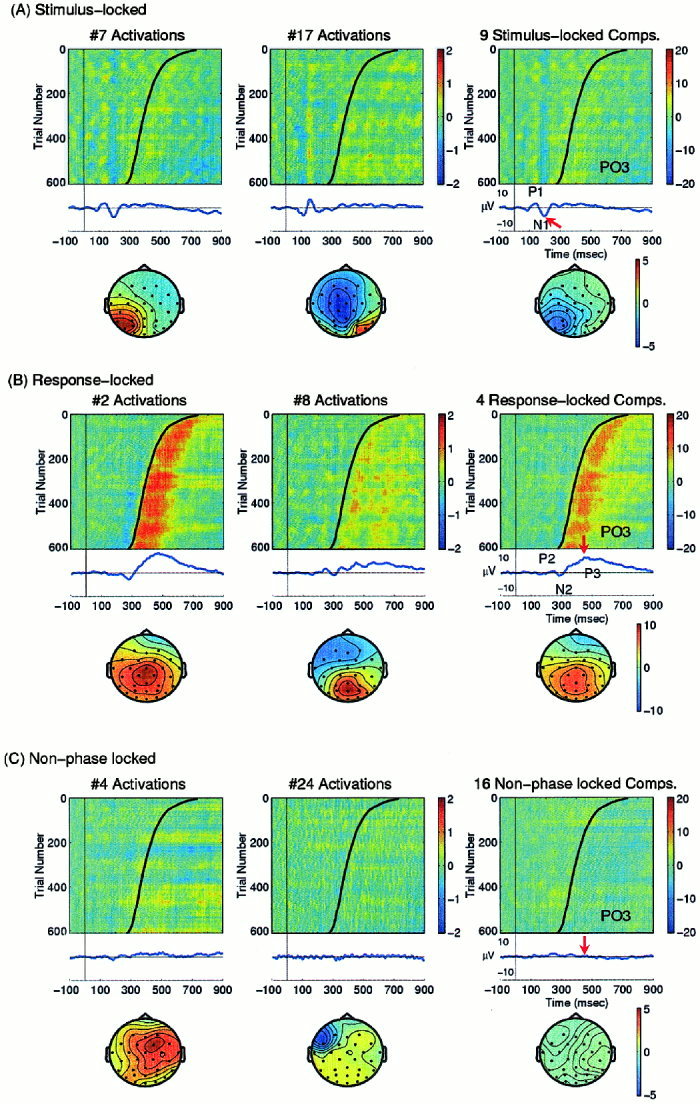
Three categories of ICA components of single‐trial ERP data. (Left) RT‐sorted ERP images of selected ICA component activations and scalp maps, and (right) their summed projections onto a left posterior scalp site (PO3) of the autistic subject. Smoothing width in all images: 30 trials. (A, left) Single‐trial activations of two of nine independent components accounting for stimulus‐locked activity. Mean activation shown below (relative units). (Right) Summed projection, at left posterior site PO3, of all nine independent components accounting for stimulus‐locked activity, with the ERP average at this site shown below (units: μV). (B, middle left) Two of four independent components accounting for response‐locked activity. (Right) Summed projection at PO3 of all four response‐locked components. (C, middle left) Two of 16 independent components accounting for non‐phase locked activity. (Right) Summed projection at PO3 of all 16 spontaneously active components.

Results of ICA decomposition

ERP images of the independent components of the target responses single‐trial data displayed a variety of features with distinct relations to task events. Because of space constraints, we illustrate these features by showing data from one 30‐year‐old male normal control subject and two (19‐ and 32‐year‐old) high‐functioning male subjects with autism, although we obtained similar results in all 50 cases.

Figure 3 shows the scalp maps and power spectra of the 31 independent components derived from 641 target response epochs from a 32‐year‐old autistic subject. Several of these components can be assigned to different component types using the procedure described in Methods. Some components clearly captured a category of non‐time locked non‐brain activity such as blinks (#1), eye‐movements (#9), or muscle artifacts (#14). Many accounted for portions of rhythmic activity (e.g., alpha #7, 8, 17, etc.). Note that some component maps were bilaterally symmetric (e.g., #24 and 29). The nature of other components was not clear from their scalp topographies and spectra (see Fig. 5). These component types are discussed separately below. The mean variance of the projections of each of the 31 independent components across the scalp electrodes is shown in Figure 3 (bottom right).

Figure 3.

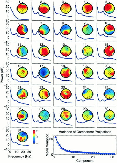
The scalp maps and power spectra of the 31 independent components derived from target response epochs from a 32‐year‐old autistic subject. Blink and eye movement artifact components (IC1 and IC9) had a typical strong low frequency peak. Temporal muscle artifact components (i.e., ICs 14, 22, 27, and 29) had characteristic focal optima at temporal sites and power plateaus at 20 Hz and higher. Some components captured oscillatory activity (i.e., ICs 7, 8, 17, etc.). Some components included features that systematically time‐ and phase‐locked to stimulus onsets or subject responses (Fig. 5).

Removing blink and eye‐movement artifacts

Figure 4 shows an example of ICA‐based artifact removal. In this example, ICA was applied to target responses collected from a 19 year‐old autistic subject performing the visual spatial selective attention experiment. Although the subject was instructed to fixate the central cross during each 72‐sec block, he tended to blink or move his eyes slightly toward target stimuli presented at peripheral locations. ICA successfully isolated blink artifacts to a single independent component (Fig. 4A) whose contributions could be removed from the EEG records by subtracting the component projection from the data [Jung et al., 1998a, 1998b, 2000a, 2000b]. A second ICA component accounted for the small horizontal eye movements (Fig. 4B).

Figure 4.

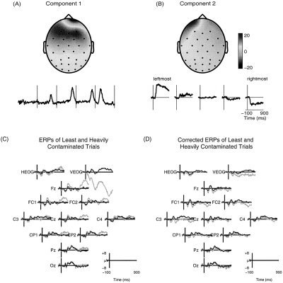
Elimination of eye‐movement artifacts from ERP data. (A) Scalp topography and five consecutive 1‐sec target response epochs showing the time course of activation of an ICA component accounting for blink artifacts. This component was separated by ICA from 321 target‐response trials recorded from an adult autistic subject in the visual selective attention experiment. (B) The scalp topography of a second eye‐movement component and its average activation time course in response to target stimuli presented at the five different attended locations. (C) Averages of (N = 231) relatively uncontaminated (solid traces) and (N = 90) heavily contaminated (faint traces) single‐trial target response epochs from a normal control subject. (D) Averages of ICA‐corrected ERPs for the same two trial subgroups overplotted on the average of uncorrected uncontaminated trials.

A standard approach to ERP artifact rejection is to discard eye‐contaminated trials containing maximal potentials exceeding some selected value (e.g., 70 μV) at periocular sites. For this data set, this procedure rejected 90 of 321 or 28% trials of the subject's data. For the data set collected from one of the lesion subjects, the same procedure would have rejected over 60% of trials. Figure 4C shows the ERP averages of the relatively uncontaminated target trials (solid traces) and the heavily contaminated target trials (faint traces) that would have been rejected by this method. Note that the averages of these two groups of trials differed most at frontal electrodes. Figure 4D shows averages of the same uncontaminated (solid traces) and contaminated (faint traces) trials after the ICA components accounting for the artifacts were identified and removed, and the remaining components projected back onto the scalp electrodes. The two ICA‐corrected averages were almost completely coincident, showing that ICA‐based artifact removal did not change the neural signals that were not contaminated. Note that the “ICA‐corrected” averages of these two trial groups are remarkably similar to the average of the uncontaminated trials before artifact removal (Fig. 4C, solid trace). This implies that the corrected recordings contained only event‐related neural activity and were free of artifacts arising from blinks or eye movements.

Similar ICA‐based artifact removal was applied to single‐trial target‐response records from all 28 normal, ten autistic, and 12 brain lesion subjects in this experiment. Artifact‐removal results for remaining 49 subjects were at least as impressive as in Figure 4. More examples and supporting evidence can be found in Jung et al. [2000b] and online at http://www.cnl.salk.edu/~jung/ERPartifact.html.

Stimulus‐locked activity

Single‐trial EEG records include ongoing EEG that are not time‐locked and/or phase‐locked to experimental events. Applied to the single‐trial EEG records, ICA identified stimulus‐locked, response‐locked, and non‐phase locked response features in mostly separate classes of independent components. The numbers of components in each class varied between subjects. This is illustrated further by the ICA decomposition of the EEG data from a 32‐year‐old autistic subject, the same subject shown in Figure 3. After removal of two ICA components (IC1 and IC9) accounting for blinks and eye movements (similar to those in Fig. 4), 29 ICA components remained.

Figure 5A (middle left) shows single‐trial activations of two of nine ICA components accounting for portions of the stimulus‐locked response activity. Note that both the response latencies and active durations of the early stimulus‐locked P1 and N1 components were stable and time‐locked to stimulus onsets in nearly all trials. Each of these nine independent components had distinct time courses. For example, the peak latency (156 msec) of the early N1‐latency component extracted by IC17 (middle) led that of the late N1 activity (195 ms) accounted for by IC7 (left). The scalp maps of the two components were distinct, although overlapping and non‐orthogonal (r = 0.09). The maps of these two components resemble the N1a and N1b components separated by ICA from the set of normal‐subject grand mean ERPs in these experiments [Makeig et al., 1999b]. Details of the early single‐trial visual response components will be reported elsewhere.

The single‐trial activations of nine stimulus‐locked components were projected back onto the scalp channels and then summed to estimate their contributions to the averaged response. Figure 5A (right) shows the summed projections, at the left posterior site PO3, accounting for nearly all of the P1 and N1 peaks in the raw response waveform but for only part of the P2 and N2 response peaks. The scalp map of the summed projections at the N1 peak (195 msec) is shown below the ERP image. The ICA separation of P2/N2 activity into both stimulus‐locked and response‐locked components may explain the often‐noted difficulty in characterizing the nature and sources of these intermediate response peaks.

Response‐locked activity

Figure 5B (left, middle) shows activations of two of the four ICA components accounting primarily for response‐locked activity. The activations of these components had distinct relationships to subject responses. Peak latencies of the response‐locked activity covaried with response time, while their active durations were stable. Figure 5B (right) shows the summed projections of these four ICA components at left parietal‐occipital site PO3, and the scalp map of their summed projections at the “P3” peak (453 msec) in their response average. Note that response latency differences produced a pronounced temporal smearing of the P3 peak in the averaged ERP (middle right), yielding an inaccurate average of event‐related brain responses to target stimuli. Peaks in averaged ERPs have been the primary features used to study brain dynamics surrounding experimental events. Inaccuracies of ERP averaging might lead to mistaken conclusions based on inaccurate peak amplitudes and latencies. Below we describe an effective method for realigning these single‐trial event‐related activities while preventing temporal smearing.

Spontaneous EEG activity

For the same subject, the remaining non‐phase locked background EEG activity was accounted for by 16 components, several of which were quite small. The single‐trial activations of two of these components and the summed projection of all 16 components at site PO3 are shown in Figure 5C. As expected, because of phase cancellation induced by averaging 641 trials, the summed projections of ICA components accounting for non‐phase locked background EEG activity contributed very little to the ERP average (Fig. 5C, bottom right trace). The scalp map of their summed projections at the (453 ms) “P3” peak latency (bottom right) does not resemble that of the “P3” response in the averaged ERPs (Fig. 5B, right).

Realigning single‐trial ERPs

Figure 6A (top left) shows the artifact‐corrected single‐trial ERP epochs at left posterior site PO3 for the same subject (i.e., the sum of the data shown in the rightmost ERP‐image panels of Fig. 5). The latency of the N1 peak (dotted line) was stable across trials, whereas response latency differences in long‐ and short‐RT trials produced a pronounced temporal smearing of the P3 peak in the averaged ERP (bottom trace), giving an inaccurate representation of event‐related brain response to target stimuli. Realigning the single‐trial ERP epochs to the median reaction time (top right) sharpened the averaged P3, but unfortunately smeared out the early stimulus‐locked activity across trials (dotted line), thus removing the early (100–300 msec) response peaks from the averaged response (bottom trace). However, because ICA separated much of the stimulus‐locked, response‐locked and non‐phase locked background activity into different subsets of independent components (Fig. 6B), we could first realign the time courses of the components accounting for response‐locked ERP features (middle) to the median reaction time, (Fig. 6C, middle) and then sum them with the stimulus‐aligned projections of time courses of stimulus‐locked early components (P1, N1, etc.) (Fig. 6B, left), forming artifact‐ and latency‐corrected data that preserved the early stimulus‐locked response (P1, N1) while sharpening the response‐locked P3 (Fig. 6C, bottom right). In this record, temporal smearing in the averaged ERP arising from performance fluctuations is minimized without smearing or eliminating the stimulus‐locked components (dotted line) (compare 6A, top right, and 6C, bottom right).

Figure 6.

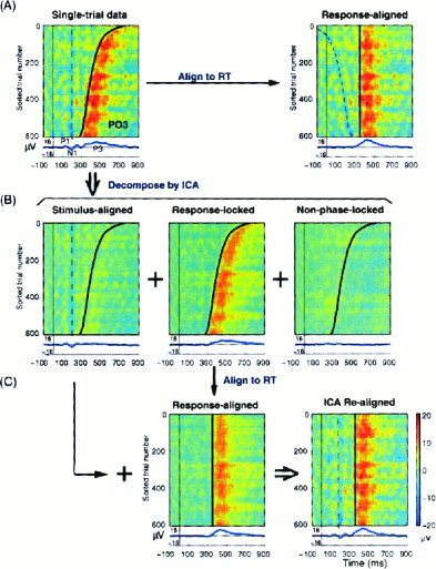
Realignment of the ERPs to compensate for variable reaction times. (A) Artifact‐corrected, RT‐sorted single‐trial ERP data for the same autistic subject at site PO3 time‐locked, respectively, to stimulus onsets (left) and to subject responses (right). Note that the early ERP features (P1, N1, etc.) are out‐of‐phase in the response‐locked trials (right) and therefore do not appear in the response‐locked average (bottom right trace). (B) The single‐trial data at PO3 were decomposed by ICA into summed projections of components accounting for (left) stimulus‐locked, (center) response‐locked, and (right) non‐phase‐locked background EEG activity. (C) Projections of the response‐locked components to site PO3 were aligned to median reaction time (355 ms) and summed with the projections to PO3 of stimulus‐locked components (B, left), forming an enhanced ICA‐aligned ERP (bottom right trace).

Classifying subtypes of endogenous ERPs

By separating event‐related responses components from background EEG processes and EEG artifacts, ICA also allowed differences in single‐trial responses to be more closely examined. This is illustrated by characterizing the relatively artifact‐free spatiotemporal P3 response extracted by ICA in each single trial response from the same autistic subject (Fig. 7). First, the time courses of the four response‐locked components accounting for the P3 were realigned to the median response time and then the response‐aligned activations were projected back to site PO3 (Fig. 7A, left). By using the average of the response‐aligned P3 waveform (bottom trace) as a template for correlating with the waveform of each single‐trial projection (left), two trial subsets were identified comprised of relatively “consistent” and “inconsistent” P3 responses, respectively. Figure 7A (middle) shows the ERP image of 515 response‐aligned consistent P3 response trials (80% of the trials), in which the P3 component activation resembled the average time course (r = 0.3). In the remaining 126 inconsistent P3 response trials (20%) (right), the response morphology differed markedly (r < 0.3) from the mean response.

Figure 7.

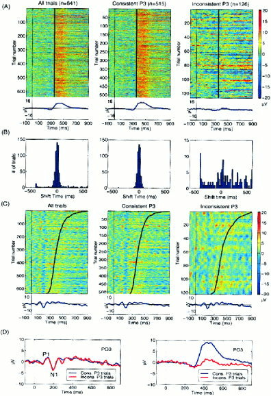
Analysis of variability in the P3 component in single trial ERPs. (A) Summed projections of the four ICA components to left‐posterior site PO3 accounting for response‐locked P3 activity (left) could be separated into 515 consistent‐P3 trials (middle), whose activations resembled those of the averaged P3‐component activation (r = 0.3), and 126 inconsistent‐P3 trials (right) (r < 0.3) whose average (bottom right trace) did not resemble the averages of the consistent trials (middle trace) or of all the trials (right trace). To better illustrate intertrial differences, the ERP images are unsmoothed. (B) Distributions of latency shifts yielding maximal correlations between the P3 template (A, bottom left trace) and each response‐aligned trial, for (left) all trials, (middle) the 515 consistent‐P3 trials, and (right) the 126 inconsistent‐P3 trials. Note that P3 waveforms of most of trials were consistently time‐locked to the subject's responses, as evidenced by a tight concentration near zero‐time shift in the left and center histograms. However, the maximally correlated shift times for the inconsistent trials (right) had no central tendency. (C) ERP images of projected stimulus‐locked activity at site PO3 for (left) all, (middle) consistent, and (right) inconsistent‐P3 trials appear similar. (D) Averages of (blue) consistent‐P3 and (red) inconsistent‐P3 trials. (Left) Summed projected stimulus‐locked components produce identical early P1/N1 response peaks at site PO3. (Right) Summed projected response‐locked components at site PO3 produce dramatically different responses for the two trial subsets.

To test the response‐locking of the activity isolated by these components, we cross‐correlated each trial (i.e., each horizontal trace in Fig. 7A, left) with the P3 template (Fig. 7A, bottom left trace). Fig. 7B shows histograms of the latency shifts giving maximal correlations for all trials (left), consistent response trials (middle), and inconsistent response trials (right). Note that most of the consistent response trials were time‐aligned to the template, as evidenced by a tight concentration near zero in the histogram (middle), implying that their peak latency consistently followed the subject response latency by about 100 msec. Note also that the outliers in the histogram of latency shifts for all trials (left vs. middle) were mainly contributed by the inconsistent response trials (Fig. 7B, right), even though the zero‐lag waveform correlation rather than the size of the time shift was used as the criterion for classifying trials as consistent or inconsistent.

An interesting and related question was whether stimulus‐locked activity differed between consistent and inconsistent response trials. Figure 7C shows ERP images of summed stimulus‐locked component activity projected to site PO3 in all trials (left), consistent response trials (middle), and inconsistent response trials (right). Stimulus‐locked activity (Fig. 7D, left) was similar in consistent and inconsistent trial subsets. However, as expected, the averages for the same two trial subsets of the summed activity of the response‐locked components differed strongly between 300 msec and 800 msec (Fig. 7D, right).

Constructing an optimized ERP average

Many studies have attempted to use peak measures of LPC or P3 waveforms to test a wide range of clinical and developmental hypotheses. By applying artifact removal, extraction of event‐related activity, response realignment, and inconsistent P3 response trial pruning to the target‐response epochs from the autistic subject, we derived an optimized target P3 (Fig. 8, solid traces). Note that, compared to the raw averaged ERP (dashed traces), the optimal P3 peak at central‐parietal site Pz had 50% larger amplitude and 20 msec shorter latency (plot insert), with a shorter active duration than the raw averaged ERP. Similar differences are apparent in Figure 8 at all central and posterior channels.

Figure 8.

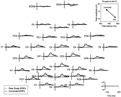
Effects of artifact and latency correction on averaged ERPs from an autistic subject. Average of all 641 single target trials from the autistic subject, before (dashed traces) and after (solid traces) artifact‐removal, latency‐realignment, and elimination of 126 inconsistent‐P3 trials from the average (see Results). The plot insert (top right) shows P3 peak latency and amplitude at site Pz before and after correction. Note the larger, earlier and narrower P3 peak in the corrected average at central and posterior channels.

Event‐related oscillatory EEG activity

ICA applied to multichannel single‐trial EEG records can also separate multiple, spatially overlapping oscillatory components, even when they have maximal energy within the same frequency band [Makeig et al., 1996]. For example, Figure 9 plots the ERP images and scalp topographies of activations of two ICA components accounting for alpha‐band (8–12 Hz) activity in target‐response epochs from a 30‐year‐old normal control subject. Note that alpha activity in the activation average of the central occipital component (left, bottom trace and scalp map) seemed augmented in the averaged response following stimulation, whereas alpha activity in the right‐central component (middle and scalp map) was clearly reduced or blocked at or before the subject response (black trace). The peak alpha frequencies in the single‐trial activations of the two components were near identical (circa 11 Hz), yet because of time‐varying differences in amplitude and phase their activations were nearly uncorrelated (r = 0.002). The power spectrum (not shown) of the second component contained a second peak near 20 Hz, whereas the spectrum of the first component did not. The spectra, scalp maps, equivalent dipole source locations (not shown), and activity blocking following the button press are all compatible with the behavior of the EEG mu rhythm associated with the motor system [Kuhlman, 1978; Makeig et al., 2000b; submitted]. When the ICA component filter for the right mu component was applied to data from a second session in which the same subject was instructed to attend to target stimuli without making a button press (right panel), this component was again recovered but its rhythmic alpha‐band activity was not blocked.

Figure 9.

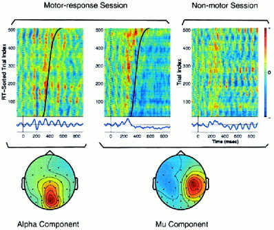
Non‐phase locked ICA components with and without event‐related dynamics. (Top left and middle) ERP images of single‐trial activations of two ICA components accounting for alpha activity in single trials from a normal control subject, and their scalp topographies. Images smoothed with a 30‐trial moving window. The separate alpha activities accounted for by these components were respectively enhanced (left) or blocked (middle) by subject responses. When the spatial filter for the second alpha component (middle) was applied to single target trials from another session in which the same subject was asked only to “mentally note,” but not physically respond to targets (right), this component's alpha activity was not blocked.

Conversely, when ICA was trained on target response trials from the no‐response session, it derived a spatial filter nearly identical to the right mu component (scalp maps r = 0.94). When the new spatial filter was applied to the trials from the motor‐response session, the component's alpha activity again was blocked following the response, even though the new component was derived from the non‐motor response session in which the activity was not blocked. This result indicates that ICA can extract the activity of distinct, spatially distributed alpha‐band activities that may be differently affected (or unaffected) by stimulus presentation and/or subject responding. Details of these and other oscillatory components will appear elsewhere [Makeig et al., submitted].

Component stability

Component scalp maps and activation spectra of 713 (31 × 23) independent components from 23 normal control subjects (aged between 16 and 80, mean: 44.8, 14 males and nine females) were clustered using a symmetrical Mahalanobis distance measure (see Methods and Appendix). Of the resulting clusters, several accounted for eye blinks (Fig. 10A, left), lateral eye movements (middle), and temporal muscle activity (right), as judged by their scalp maps, mean spectra, and activity patterns in single trials. These artifactual components were separated from nearly every subject's data.

Figure 10.

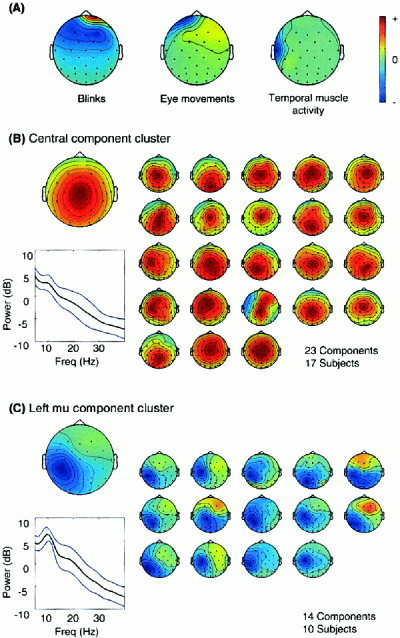
Between‐subject component stability. (A) Three stable component clusters accounting for blinks (N = 27/23 Ss), eye movements (N = 19/16 Ss) and left temporal muscle activity (N = 19/16 Ss). These components were near‐perfectly replicated across all subjects. (B) The largest nonartifactual component cluster (N = 23/17 Ss). (Leftmost map) Mean component map. (Bottom) Mean power spectra (red) ± SD. The components account for much of the LPC. Individual maps in this cluster resembled the cluster mean map (leftmost). (C) Left mu rhythm component cluster (N = 14 / 10 Ss). Note the spectral peaks near 11 and 20 Hz. The activations of these components were significantly reduced following the response period between 500 to 1000 msec after stimulus onset.

The largest two clusters not accounting for artifacts are shown in Figure 10B and C. Figure 10B shows the mean map and power spectrum of a large cluster of central parietal components. In this cluster, the component activations accounted for a portion of the vertex‐positive “P3”. Twenty‐three components from 17 subjects were grouped into this cluster. The power spectra of the component cluster in Figure 10C contained peaks near 11 and 20 Hz. In all 14 components from ten subjects contributing to this cluster, the 11‐Hz activity was significantly blocked following subject responses as in Figure 9 (middle), strongly suggesting these represented mu activity [Kuhlman, 1978; Makeig et al., submitted]. Scalp maps of individual left mu components in this cluster strongly resembled the (left) cluster mean map. Nine subjects contributed one component to this cluster, three subjects contributed two components, and one subject contributed three. Table I summarizes largest component clusters, number of components in the each cluster, and the number of contributing subjects out of a total of 23 subjects.

Table I.

Major component clusters

	Eye		Temporal muscle		Posterior α			mu		Central occipital α
Activity type	Blink	Eye movement	Left	Right	Left	Right	“P3”	Left	Right
Number of components	27	19	19	11	13	13	23	14	10	12
Number of contributing subjects	23/23 100%	16/23 70%	16/23 70%	9/23 39%	10/23 43%	12/23 52%	17/23 74%	10/23 43%	8/23 35%	9/23 39%

The results of component clustering. The activity accounted for by the 10 largest component clusters, numbers of individual components participated in the each cluster, and numbers of subjects having components in the clusters are shown here. The mean scale maps of three largest artifactual components clusters and two largest non‐artifactual, P3b and left mu, are shown in Figure 10.

DISCUSSION

In this study, ICA was applied to single‐trial target‐response records from 22 neurological patients and 28 adult control subjects in a visual selective attention experiment, producing for each subject 31 maximally independent EEG components having a variety of distinct relations to task events. Some components included activity time‐ and phase‐locked to stimulus onsets thereby accounting for a portion of the stimulus‐locked ERP. Others included activity time‐ and phase‐locked to subject responses, thereby accounting for a portion of the response‐locked ERP. Still other components accounted for blinks, eye movements, muscle noise, and EEG activity not locked either to stimuli or responses.

Our confidence in the usefulness of ICA decomposition of EEG signals is strengthened by these results: first, by its apparently clean separation of eye blink and eye movement artifacts and, second, by the physiologically plausible scalp maps of all but the smallest ICA components. Scalp maps of larger components tended to have few spatial optima, consistent with relatively simple source generators. Elsewhere, we have presented further evidence for the robustness of ICA decomposition applied to ERP averages [Makeig et al., 1997, 1999a, 1999b, 2000c].

Artifactual components

ICA‐based artifact removal can effectively detect and separate contaminations arising from a wide variety of artifactual sources in EEG records without sacrificing neural signals recorded at sites most affected by the artifacts. This method also can preserve most or all of the recorded trials for analysis, even when few if any of the raw trials are artifact‐free.

Researchers have recognized the importance of single trials as reflecting dynamic operations such as orienting, habituation, or associative learning. However, they typically have had to sacrifice some or most of the information contained in single trials to increase the signal‐to‐noise ratio by averaging single trials across subjects [Kenemans et al., 1989] or across time intervals [Courchesne et al., 1978]. Making use of information about single trials while removing artifacts with ICA may help researchers to take fuller advantage of what until now has been an only partially realized strength of ERP paradigms—the ability to examine systematic msec‐scale variations from trial to trial within subjects.

Exogenous and endogenous components

ERP researchers have traditionally distinguished between shorter‐latency exogenous components, whose amplitudes and/or latencies depend directly on physical characteristics of the evoking stimulus, and longer‐latency endogenous components whose size and latency depend on the cognitive relevance of the stimulus [Goodin et al., 1986]. ERP images both of single‐trial raw data and of its independent component activations (Fig. 5) have revealed that in our experiments the later (“endogenous”) P3 components were clearly time‐locked to the motor responses, whereas early (“exogenous”) P1, N1 components were reliably time‐locked to stimulus onsets. ICA decomposition makes possible the study of properties of exogenous and endogenous response activities in single trials. The independence of stimulus‐locked and response‐locked activities in consistent and inconsistent P3 trials (Fig. 7) demonstrates that different factors modulate the amplitudes of these two component classes. The ability of ICA to study relationships between exogenous and endogenous activity in each trial could open new basic and clinical research opportunities.

Response latency variability

Using ERP images to visualize component activations revealed response information not obtainable from response averages. In our data, response latencies and active durations of the early stimulus‐locked P1 and N1 peaks were stable in nearly all trials, whereas the later LPC or P3 peak covaried with response time (i.e., it was response‐locked). ICA separated stimulus‐ and response‐locked event‐related activity into different components on the basis of temporal independence and differences in spatial distribution. ICA allowed the time courses of response‐locked components to be realigned, preventing temporal smearing of late response activity in the average.

Examining single‐trial activations of response‐locked independent components made it easy to classify subtypes of ERP trials by reducing confounds from large artifacts and nontask‐related background EEG activity. Although P3 response amplitudes and wave shapes varied widely from trial to trial, latency variability in late positive complex of responses to visual targets could be explained nearly entirely by a small set of independent components that were consistently time‐locked to the subject's motor responses. Reasons for the trial‐to‐trial performance differences might arise from intertrial differences in attention or arousal, or be linked to differences in the stimulus sequences preceding target presentation. Alternatively, they might arise from the subject using different strategies to perform the same task, even within the same session. Using the methods presented here, these and other possibilities can now be studied in detail.

Optimal response averaging

The ICA‐adjusted ERP averages derived for each subject represented time‐ and phase‐locked event‐ related brain activity more faithfully than either the stimulus‐ or response‐aligned averaged ERPs because: (1) the trials were relatively artifact‐free; (2) response‐locked features of the ERP were aligned to the median subject response time, thereby minimizing temporal smearing included by stimulus‐aligned averaging; (3) approximately 20% of target response trials contained little or no P3 activity that were not included in the average. When peak measures applied to ERP averages are used to index response dynamics associated with experimental manipulations, ICA optimization can remove pervasive artifacts, realign the response‐locked activity to prevent temporal smearing, and give information useful for pruning deviant trials, thereby more faithfully representing the average responses of interest. Such enhanced averaging has long been a goal of ERP signal processing efforts (e.g., Wiener‐filtered ERPs) [Woestenburg et al., 1983b].

Background EEG components

The summed projections of ICA components accounting for non‐phase locked (or “background”) EEG activity contributed little to the averaged ERP. However, the ICA decomposition reveals the brain dynamics of spatiotemporally overlapping components of spontaneous brain activity that were distinctively affected by experimental events. ICA identified multiple oscillatory EEG components with spectral peaks at a range of frequencies. At alpha band frequencies (8–12 Hz), multiple independent components with differing scalp topographies were found in single‐trial responses. The time courses of activation of these components proved to be consistently and distinctively affected by task events. Observed event‐related modulations in these (and other) data included event‐related amplitude augmentation or blocking time locked to target‐stimulus onsets or to subject responses.

Spontaneous EEG activity has been analyzed primarily in the frequency domain, most often using measures of power in standardized frequency bands such as theta (4–7 Hz) and alpha (7–12 Hz). Event‐related depressions in spectral power in the alpha band have been studied for nearly 30 years as “event‐related desynchronizations” (ERDs) [Pfurtscheller et al., 1979]. More recently, full‐spectrum event‐related changes in spectral power, termed “event‐related spectral perturbations” (ERSPs) have been demonstrated [Makeig, 1993]. Event‐related changes in phase coherence between signals collected at pairs of scalp channels have also been reported [Rappelsberger et al., 1994; Sarnthein et al., 1998; Walter, 1968]. However, both power and coherence studies use as their unit of analysis relatively narrow frequency bands at single scalp channels or channel pairs, even though most neural generators of oscillatory activity project widely across the scalp, making each scalp channel report the sum of multiple neural sources. Also, these time‐frequency methods rely on averaging across large numbers of trials, and are thereby also subject to contamination by artifacts.

ICA, on the other hand, identifies spatially‐overlapping patterns of coherent activity over the entire scalp and frequency pass band rather than focusing on activity at single frequencies in single scalp channels or channel pairs. Unlike ERP averaging, which acts on oscillatory activity like a comb‐filter, passing only activity both time‐ and phase‐locked to experimental events, ICA allows phase and timing of oscillatory activity to vary independently within identified sources. Because ICA segregates different spatial patterns of oscillatory activity into different components, it facilitates the study of event‐related modulations, compared to studying these modulations at single scalp electrodes, which inevitably record the activity of multiple functional brain sources generated within a large brain area. ICA also separates oscillatory components from overlapping artifactual activity.

Component stability

We previously reported the component stability of ICA decomposition of single‐trial 1‐sec EEG epochs on two different levels: the replicability of components obtained from repeated ICA training on the same data set, and our previous results [Jung et al., 2000a; Makeig et al., 1997, 1999a]. These results showed that ICA decomposition is relatively insensitive to the exact choice of learning rate or batch size. In repeated trainings with the data delivered to the training algorithm in different random time orders, independent components with large projections were unchanged, though the smallest components typically varied.

Within‐subject spatiotemporal stability of independent components was tested by applying moving‐window ICA to sets of overlapping event‐related sub‐epochs of the same single‐trial recordings used in this study [Makeig et al., 2000a, submitted]. Our results showed that ICA decomposition of multichannel single‐trial event‐related EEG data could give stable and reproducible information about the spatiotemporal structure and dynamics of the EEG before, during, and after experimental events. In addition, component clusters produced by single ICA decompositions of sets of whole target‐stimulus epochs strongly resembled those produced by moving‐window decompositions.

Here we investigated the between‐subject stability of independent components of the single‐trial 1‐sec EEG epochs by applying a component clustering analysis (component‐matching approach based on the component scalp maps and power spectra of component activations) of 713 components derived from 23 normal controls. We found that clusters accounting for eye blinks, lateral eye movement, and temporal muscle activities were detected by ICA in almost all subjects. In general, clusters accounting for event‐related activity including early stimulus‐locked activity, late response‐locked activity (P3), event‐modulated mu, and alpha band activities were largely replicated in many subjects, whereas components accounting for non‐phase locked EEG activities varied across subjects.

Differences in single‐trial ERPs between normal controls and neurological patients

The difference in single‐trial ERPs between the normal controls and neurological patients can be investigated using ERP image plots. Although we do not yet have enough subjects to generalize across these two patient populations, preliminary results are quite interesting. Townsend et al. [2001] found that single‐trial variability of average “P3” amplitude at Pz was larger for control subjects than for autism subjects. Control subjects generated “P3” responses that were greater than 5 μV on approximately two‐thirds of the single trials, whereas autism subjects generated responses that large on only one‐third of the single trials. In a study of comparing ERPs in normal patients and cerebellar lesion patients, Westerfield et al [unpublished] showed that although the control subjects had robust “P3” activity time locked to button press, lesion subjects had weaker, sporadic poststimulus positive activity. Further studies on subjects from these subject groups will be reported separately.

ICA limitations

Although ICA seems to be generally useful for EEG analysis, it also has some inherent limitations: First, ICA can decompose at most N sources from data collected at N scalp electrodes. Usually, the effective number of statistically‐independent signals contributing to the scalp EEG is unknown, and it is likely that observed brain activity arises from more physically separable effective sources than the available number of EEG electrodes. To explore the effects of a larger number of sources on the results of the ICA decomposition of a limited number of available channels, we ran a number of numerical simulations in which selected signals recorded from the cortex of an epileptic patient during preparation for operation for epilepsy were projected onto simulated scalp electrodes using a three‐shell spherical model [Makeig et al., 2000c]. We used electrocorticographic data in these simulations as a plausible best approximation to the temporal dynamics of the unknown EEG brain generators.

Results confirmed that the ICA algorithm can accurately identify the time courses of activation and the scalp topographies of relatively large and temporally‐independent sources from simulated scalp recordings, even in the presence of a large number of simulated low‐level source activities. In many decompositions, the largest ICA components were highly stable, with similar topographies and time courses across subjects, whereas the smallest ICA components appeared noisy (i.e., were variable between subjects and repeated trainings and/or had complicated scalp topographies, or else accounted predominantly for artifacts in a few “outlier” epochs). Thus, independent components making small contributions to the scalp data and having complex scalp maps, may represent mixtures of many small brain sources, and should be interpreted cautiously.

Second, the assumption of temporal independence used by ICA cannot be satisfied when the training data set is too small, or when separate topographically distinguishable phenomena nearly always co‐occur in the data. In the latter case, simulations show that ICA may derive single components accounting for the co‐occurring phenomena, along with additional components accounting for their brief periods of separate activation. Such confounds imply that behavioral or other experimental evidence must be obtained before concluding that ICA components with spatiotemporally overlapping projections are functionally distinct. This report illustrates two such criteria: independent components may be considered functionally distinct when they exhibit distinct reactivities to experimental events (Fig. 9), or when their activations correspond to otherwise observable signal sources (Fig. 4).

Third, ICA assumes that physical sources of artifacts and cerebral activity are spatially fixed over time. In general, there is no reason to believe that cerebral and artifactual sources in the spontaneous EEG might not move over time. Examples of spatially fluid sources may include spreading sleep spindles [McKeown et al., 1998], as suggested by neurophysiological modeling [Bazhenov et al., unpublished]. However in our data, the relatively small numbers of components in the stimulus‐locked, response‐locked, and non‐phase locked categories, each accounting for activity occurring across sets of 500 or more 1‐sec trials, suggests that the ERP features of our data were primarily stationary, consistent with repeated observations in functional brain imaging experiments that discrete and spatially restricted areas of cortex are activated during task performance [Friston et al., 1998].

CONCLUSIONS

The study of single‐trial event‐related brain responses has been frustrated for decades by problems of dealing simultaneously with eye and muscle artifacts, spontaneous EEG sources, and spatiotemporally overlapping response components. This paper demonstrates promising analytical and visualization methods for multichannel single‐trial EEG recordings that may overcome these problems.

The ERP image (or, applied to MEG data, the event‐related field or “ERF image”) makes visible systematic relations between experimental events and single‐trial EEG (or MEG) records, and their ERP (ERF) averages. ERP images can also be used to display relationships between phase, amplitude, and timing of event‐related EEG components that are time‐locked either to stimulus onsets, to subject responses, or to other parameters. Applied to these data, they revealed that latency variability in visual target‐evoked responses is predominantly accounted for by response‐locked activity. The ERP image can be used to display single‐trial raw data (Fig. 2) and their independent component activations (Fig. 5).

Independent component analysis of single‐trial ERP data allows blind separation of multichannel complex EEG data into a sum of temporally independent and spatially fixed components. Our results show that ICA can separate artifactual, stimulus‐locked, response‐locked, and non‐event related background EEG activities into separate components, allowing: (1) removal of pervasive artifacts of all types from single‐trial EEG records, making possible analysis of highly contaminated EEG records from clinical populations, (2) identification and segregation of stimulus‐ and response‐locked EEG components, (3) realignment of the time courses of response‐locked components to prevent temporal smearing in the average, (4) classification of response subtypes, and (5) separation of spatially‐overlapping EEG activities that may show a variety of distinct relationships to task events.

Component‐matching clustering analysis automatically grouped components from 23 normal controls having similar scalp maps and power spectra. The results showed that components accounting for blink, eye movements, temporal muscle activity, event‐related activity, and event‐modulated mu and alpha activities were similar across subjects.

Better understanding of trial‐to‐trial changes in brain responses may allow a better appreciation of the limitations of normal human performance in repetitive task environments, and may allow more detailed study of changes in cognitive dynamics in brain‐damaged, diseased, or genetically abnormal individuals. The proposed methods also allow the investigation of the interaction between ERPs and ongoing EEG. The analysis and visualization tools proposed in this study seem to enhance the amount and quality of information in event‐ or response‐related brain signals that can be extracted from ERP data, and so seem broadly applicable to electrophysiological research on normal and clinical populations.

COMPONENT CLUSTERING

Clustering Extraction of dominant scalp activity maps from multiple subjects requires a method that can cope with the expected large fraction of outlier elements. These include two general classes of maps: A map located near but not within a map cluster (an outlier of the cluster), else a map situated far from any cluster (an outlier of the map collection). To determine cluster densities, a distance measure is required. In statistical analysis, a frequently used measure is the Mahalanobis distance [Bishop, 1995], which linearly rotates the data by the data covariance matrix. The process is analogous to pre‐whitening of the data. Unlike the Euclidian distance measure, the Mahalanobis distance increases sensitivity in directions of the data space having high sample densities while allowing more tolerance in sparse directions. Dense regions may contain closely situated but distinct clusters that simple Euclidean distance‐based clustering techniques would fail to separate.

Map signs have no meaning for oscillatory EEG components. Hence, to perform clustering on maps similar maps of opposite signs had to be jointly clustered. This requirement dictated a modification of the definition of the Mahalanobis distance (Δ) [Enghoff, 1999, p. 26]. Theoretically, no upper bound on the generated distances exists. To bound distances, measurements were mapped by the transformation Q_ij = [sign(Δ(x_i,x_j)) exp(−|Δ(x_i,x_j)|)] into the range [0,1].

The inverse‐distance matrix Q contained pairwise measurements for all possible permutations of the elements in the considered data set. After eliminating the undefined diagonal elements of Q, clusters were synthesized. The first clustering step determined the element k whose corresponding column in Q had the largest sum of inverse distances. Elements resembling the kth element at inverse‐distances above a designated threshold were jointly assigned to produce a cluster. In the second step, the clustered elements were rejected from the collection of unassigned elements together with a selection of outlier elements located in the immediate vicinity of the cluster, designated by a second threshold. These steps were repeated until either a maximum number of clusters had been found, all elements were clustered or rejected, or subsequent matches fell below a significance threshold. Thresholds used were determined by trial and error to give the largest number of clusters and best within‐cluster similarity.

REFERENCES

- Amari S, Cichocki A, Yang H (1996): A new learning algorithm for blind signal separation, In: Touretzky D, Mozer M, Hasselmo M, editors. Adv Neural Inf Proc Syst 8: 757–763. [Google Scholar]
- American Psychiatric Association (1987). Diagnostic and statistical manual of mental disorders (3rd Ed., revised). Washington, DC: American Psychiatric Association. [Google Scholar]
- Bell AJ, Sejnowski TJ (1995): An information‐maximization approach to blind separation and blind deconvolution. Neural Comput 7: 1129–1159. [DOI] [PubMed] [Google Scholar]
- Bishop C (1995): Neural networks for pattern recognition. Oxford: Clarendon Press. [Google Scholar]
- Brandt ME (1997): Visual and auditory evoked phase resetting of the alpha EEG. Int J Psychophysiol 26: 285–298. [DOI] [PubMed] [Google Scholar]
- Brandt ME, Jansen BH, Carbonari JP (1991): Pre‐stimulus spectral EEG patterns and the visual evoked response. Electroencephalogr Clin Neurophysiol 80: 16–20. [DOI] [PubMed] [Google Scholar]
- Cardoso J‐F, Laheld B (1996): Equivariant adaptive source separation. IEEE Trans Signal Proc 45: 434–444. [Google Scholar]
- Comon P (1994): Independent component analysis—a new concept? Signal Proc 36: 287–314. [Google Scholar]
- Courchesne E, Courchesne RY, Hillyard SA (1978): The effect of stimulus deviation on P3 waves to easily recognized stimuli. Neuropsychologia 16: 189–199. [DOI] [PubMed] [Google Scholar]
- Enghoff S (1999): Moving ICA and time‐frequency analysis in event‐related EEG studies of selective attention. Institute for Neural Computation Technical Report INC‐9902, University of California San Diego, La Jolla, CA.
- Florian G, Andrew C, Pfurtscheller G (1998): Do changes in coherence always reflect changes in functional coupling? Electroencephalogr Clin Neurophysiol 106: 87–91. [DOI] [PubMed] [Google Scholar]
- Friston KJ, Fletcher P, Josephs O, Holmes A, Rugg MD, Turner R (1998): Event‐related fMRI: characterizing differential responses. Neuroimage 7: 30–40. [DOI] [PubMed] [Google Scholar]
- Goodin DS, Aminoff MJ, Mantle MM (1986): Subclasses of event‐related potentials: response‐locked and stimulus‐locked components. Ann Neurol 20: 603–609. [DOI] [PubMed] [Google Scholar]
- Haig AR, Gordon E (1998): EEG alpha phase at stimulus onset significantly affects the amplitude of the P3 ERP component. Int J Neurosci 93: 101–115. [DOI] [PubMed] [Google Scholar]
- Haig AR, Gordon E, Rogers G, Anderson J (1995): Classification of single‐trial ERP sub‐types: application of globally optimal vector quantization using simulated annealing. Electroencephalogr Clin Neurophysiol 94: 288–297. [DOI] [PubMed] [Google Scholar]
- Hillyard SA, Galambos R (1970): Eye‐movement artifact in the CNV. Electroencephalogr Clin Neurophysiol 28: 173–182. [DOI] [PubMed] [Google Scholar]
- Jung T‐P, Humphries C, Lee T‐W, Makeig S, McKeown MJ, Iragui V, Sejnowski TJ (1998a). Extended ICA removes artifacts from electroencephalographic Data. In: Adv Neural Inf Proc Syst 10: 894–900. [Google Scholar]
- Jung T‐P, Humphries C, Lee T‐W, Makeig S, McKeown MJ, Iragui V, Sejnowski TJ (1998b): Removing electroencephalographic artifacts: comparison between ICA and PCA. In: Neural Networks Signal Proc VIII: 63–72.
- Jung T‐P, Makeig S, Westerfield M, Townsend J, Courchesne E, and Sejnowski TJ (1999): Analyzing and visualizing single‐trial event‐related potentials. In: Adv Neural Inf Proc Syst 11: 118–124. [Google Scholar]
- Jung T‐P, Makeig S, Humphries C, Lee T‐W, McKeown MJ, Iragui V, Sejnowski TJ (2000a): Removing electroencephalographic artifacts by blind source separation. Psychophysiology 37: 163–178. [PubMed] [Google Scholar]
- Jung T‐P, Makeig S, Westerfield M, Townsend J, Courchesne E, Sejnowski TJ (2000b): Removal of eye activity artifacts from visual event‐related potentials in normal and clinical subjects. Clin Neurophys 111: 1745–1758. [DOI] [PubMed] [Google Scholar]
- Jung T‐P, Makeig S, McKeown MJ, Bell AJ, Lee T‐W, Sejnowski TJ (2001): Imaging brain dynamics using independent component analysis. Proc IEEE 89(7): 1107–1122. [DOI] [PMC free article] [PubMed] [Google Scholar]
- Jutten C and Herault J (1991): Blind separation of sources I. An adaptive algorithm based on neuromimetic architecture. Signal Processing 24: 1–10. [Google Scholar]
- Kenemans JL, Verbaten MN, Roelofs JW, Slangen JL (1989): “Initial‐” and “change‐orienting reactions”: an analysis based on visual single‐trial event‐related potentials. Biol Psychol 28: 199–226. [DOI] [PubMed] [Google Scholar]
- Kolev VN, Yordanova JY (1997): Analysis of phase‐locking is informative for studying event‐related EEG activity. Biol Cybernet 76: 229–235. [DOI] [PubMed] [Google Scholar]
- Kuhlman WN (1978): EEG feedback training: enhancement of somatosensory cortical activity. Electroencephalogr Clin Neurophysiol 45: 290–294. [DOI] [PubMed] [Google Scholar]
- Kutas M, McCarthy G, Donchin E (1977): Augmenting mental chronometry: the P300 as a measure of stimulus evaluation time. Science 197: 792–795. [DOI] [PubMed] [Google Scholar]
- Lee T‐W, Girolami M, Sejnowski TJ (1999): Independent component analysis using an extended infomax algorithm for mixed sub‐Gaussian and super‐Gaussian sources. Neural Comput 11: 606–633. [DOI] [PubMed] [Google Scholar]
- Lord C, Rutter M, Le Couteur A (1994): Autism Diagnostic Interview‐Revised: a revised version of a diagnostic interview for caregivers of individuals with possible pervasive developmental disorders. J Aut Dev Disord 24: 659–685. [DOI] [PubMed] [Google Scholar]
- Makeig S (1993): Auditory event‐related dynamics of the EEG spectrum and effects of exposure to tones. Electroencephalogr Clin Neurophysiol 86: 283–293. [DOI] [PubMed] [Google Scholar]
- Makeig S, Galambos R (1982): Attending or discriminating 40‐Hz modulated tones induces phase‐locked subharmonic resonances in EEG. Psychopharmacol Bull 18: 55–58. [Google Scholar]
- Makeig S, Bell AJ, Jung T‐P, Sejnowski TJ (1996): Independent component analysis of electroencephalographic data. In: Adv Neural Inf Proc Syst 8: 145–151. [Google Scholar]
- Makeig S, Jung T‐P, Bell AJ, Ghahremani D, Sejnowski TJ (1997): Blind separation of event‐related brain responses into independent components. Proc Natl Acad Sci USA 94: 10979–10984. [DOI] [PMC free article] [PubMed] [Google Scholar]
- Makeig S, Westerfield M, Jung T‐P, Covington J, Townsend J, Sejnowski TJ, Courchesne E (1999a): Independent components of the late positive response complex in a visual spatial attention task. J Neurosci 19: 2665–2680. [DOI] [PMC free article] [PubMed] [Google Scholar]
- Makeig S, Westerfield M, Townsend J, Jung T‐P, Courchesne E, Sejnowski TJ (1999b): Independent components of early event‐related potentials in a visual spatial attention task. Philosophical Trans: Biol Sci 354: 1135–1144. [DOI] [PMC free article] [PubMed] [Google Scholar]
- Makeig S, Enghoff S, Jung T‐P, and Sejnowski TJ (2000a). Moving‐window ICA decomposition of EEG data reveals event‐related changes in oscillatory brain activity. The 2nd International Workshop on Independent Component Analysis and Signal Separation, 627–632.
- Makeig S, Enghoff S, Jung T‐P, Sejnowski TJ (2000b): An efficient basis for brain‐actuated control. IEEE Trans Rehab Eng 8: 208–211. [DOI] [PubMed] [Google Scholar]
- Makeig S, Jung T‐P, Ghahremani D, Sejnowski TJ (2000c): Independent component analysis of simulated ERP data. In: Nakada T, editor. Human higher function I: Advanced methodologies.
- Makeig> S, Enghoff S, Jung T‐P, Westerfield M, Townsend J, Courchesne E, Sejnowski TJ (submitted): Moving‐window independent component analysis of event‐related EEG data: component stability.
- McKeown MJ, Humphries C, Achermann P, Borbely AA, Sejnowski TJ (1998): A new method for detecting state changes in the EEG: exploratory application to sleep Data. J Sleep Res 7(Suppl. 1): 48–56. [DOI] [PubMed] [Google Scholar]
- Pfurtscheller G, Aranibar A, Maresch H (1979): Amplitude of evoked potentials and degree of event‐related desynchronization (ERD) during phonic stimulation. Electroencephalogr Clin Neurophysiol 47: 21–30. [DOI] [PubMed] [Google Scholar]
- Polich J (1997): On the relationship between EEG and P300: individual differences, aging, and ultradian rhythms. Int J Psychophysiol 26: 299–317. [DOI] [PubMed] [Google Scholar]
- Rappelsberger P, Pfurtscheller G, Filz O (1994): Calculation of event‐related coherence—a new method to study short‐lasting coupling between brain areas. Brain Topogr 7: 121–127. [DOI] [PubMed] [Google Scholar]
- Sarnthein J, Petsche H, Rappelsberger P, Shaw GL, von Stein (1998): Synchronization between prefrontal and posterior association cortex during human working memory. Proc Natl Acad Sci USA 95: 7092–7096. [DOI] [PMC free article] [PubMed] [Google Scholar]
- Scherg M (1990): Brain electric source analysis: the importance of physiological constraints. Brain Topogr 3: 268–269. [Google Scholar]
- Schopler E, Reichler RJ, De Velis RF, Daly K (1980): Toward objective classification of childhood autism: Childhood autism rating scale (CARS). J Aut Dev Disord 10: 91–103. [DOI] [PubMed] [Google Scholar]
- Small JG (1971): Sensory evoked responses of autistic children. In: Infantile Aut 224–239. [Google Scholar]
- Suwazono S, Shibasaki H, Nishida S, Nakamura M, Honda M, Nagamine T, Ikeda A, Ito J, Kimura J (1994): Automatic detection of P300 in single sweep records of auditory event‐related potential. J Clin Neurophysiol 11: 448–460. [DOI] [PubMed] [Google Scholar]
- Townsend J, Courchesne E (1994): Parietal damage and narrow “spotlight” spatial attention. J Cogn Neurosci 6: 220–232. [DOI] [PubMed] [Google Scholar]
- Townsend J, Westerfield M, Leaver E, Makeig S, Jung T‐P, Pierce K, Courchesne E (2001): Event‐related brain response abnormalities in autism: evidence for impaired cerebello‐frontal spatial attention networks. Cogn Brain Res 11: 127–145. [DOI] [PubMed] [Google Scholar]
- Verleger R, Gasser T, Möcks J (1982): Correction of EOG artifacts in event‐related potentials of EEG: aspects of reliability and validity. Psychophysiology 19: 472–480. [DOI] [PubMed] [Google Scholar]
- Walter DO (1968): Coherence as a measure of relationship between EEG records. Electroencephalogr Clin Neurophysiol 24: 282. [PubMed] [Google Scholar]
- Whitton JL, Lue F, Moldofsky H (1978): A spectral method for removing eye‐movement artifacts from the EEG. Electroencephalogr Clin. Neurophysiol 44: 735–741. [DOI] [PubMed] [Google Scholar]
- Woestenburg JC, Verbaten MN, Slangen JL (1983a): Removal of the eye‐movement artifact from the EEG by regression analysis in the frequency domain. Biol Psychol 127–147. [DOI] [PubMed] [Google Scholar]
- Woestenburg JC, Verbaten MN, Slangen JL (1983b): Stimulus information and habituation of the visual event related potential and the skin conductance reaction under task‐relevance conditions. Biol Psychol 16: 225–240. [DOI] [PubMed] [Google Scholar]
- Yabe H, Satio F, Fukushima Y (1993): Median method for detecting endogenous event‐related brain potentials. Electroencephalogr Clin Neurophysiolog 87: 403–407. [DOI] [PubMed] [Google Scholar]
- Yordanova JY, Kolev VN (1997): Developmental changes in the event‐related EEG theta response and P300. Electroencephalogr Clin Neurophysiol 104: 418–430. [DOI] [PubMed] [Google Scholar]