

Abstract
In BOLD fMRI data analysis, robust and accurate estimation of the Hemodynamic Response Function (HRF) is still under investigation. Parametric methods assume the shape of the HRF to be known and constant throughout the brain, whereas non‐parametric methods mostly rely on artificially increasing the signal‐to‐noise ratio. We extend and develop a previously proposed method that makes use of basic yet relevant temporal information about the underlying physiological process of the brain BOLD response in order to infer the HRF in a Bayesian framework. A general hypothesis test is also proposed, allowing to take advantage of the knowledge gained regarding the HRF to perform activation detection. The performances of the method are then evaluated by simulation. Great improvement is shown compared to the Maximum‐Likelihood estimate in terms of estimation error, variance, and bias. Robustness of the estimators with regard to the actual noise structure or level, as well as the stimulus sequence, is also proven. Lastly, fMRI data with an event‐related paradigm are analyzed. As suspected, the regions selected from highly discriminating activation maps resulting from the method exhibit a certain inter‐regional homogeneity in term of HRF shape, as well as noticeable inter‐regional differences. Hum. Brain Mapping 19:1–17, 2003. © 2003 Wiley‐Liss, Inc.
Keywords: BOLD fMRI, hemodynamic response function, Bayesian analysis
INTRODUCTION
Discovered in the early 1990s, functional MRI (fMRI) has quickly become the leading method to study hemodynamic changes in the brain in response to cognitive and behavioral tasks [Chen and Ogawa, 1999]. The relation between neural activity and the Blood Oxygen Level Dependent (BOLD) response is not yet clearly understood and is still under investigation [Vazquez and Noll, 1996; Buxton and Frank, 1997; Buxton et al., 1998; Li et al., 2000; Logothetis et al., 2001]. It is, therefore, convenient to model the various processes intervening in the brain, from reception of the stimulus to measurement of the BOLD contrast signal, as a whole system characterized by its transfer response function, the so‐called Hemodynamic Response Function (HRF) [Friston et al., 1994]. The HRF is the theoretical signal that BOLD fMRI would detect in response to a single, very short stimulus of unit intensity. The key assumptions related to this model are the stationarity and linearity of the underlying physiological process. Such hypotheses are good approximations of the actual properties of the system as long as the inter‐stimulus interval does not decrease below about two seconds [Dale and Buckner, 1997; Buckner, 1998].
Estimation of the HRF is a recent concern. Knowledge about the response function is believed to be a key issue to a better understanding of the underlying dynamics of brain activation and the relationship between brain areas [Biswal et al., 2000; Miezin et al., 2000]. HRFs are increasingly suspected to widely vary from region to region, from task to task, and from subject to subject [Aguirre et al., 1998; Buckner et al., 1998a,b; Miezin et al., 2000]. Unfortunately, precise and robust estimation of the HRF is still the subject of ongoing research, since the problem is badly conditioned, and various methods have been devised so far.
On the one hand, parametric methods assume that the HRF is a generally non‐linear function of certain parameters that are to be estimated. These parameters are often bestowed with some physiological meaning. Such approaches have been applied to block or event‐related stimuli. Function shapes that are typically used include Gaussian [Kruggel and von Cramon, 1999a,b; Kruggel et al., 2000] or spline‐like [Gössl et al., 2001b]. Gössl et al. [2001a] use a parametric model on the temporal scale, whereas a more general prior is used on the spatial extension of the signal. Integration of a physiological model as prior information has also been considered to constrain parametric estimation of the HRF [Friston, 2002]. But assuming the shape of the hemodynamic response to be known a priori and invariant throughout the brain is a very strong constraint, since it fluctuates greatly.
On the other hand, non‐parametric methods have been developed in an attempt to infer the HRF at each time sample. Such methods make no prior hypothesis about the shape of the response function. Since the low signal‐to‐noise ratio of fMRI data precludes direct voxelwise analysis (e.g. with averaging over time), more complex schemes have been proposed. Methods include: averaging over regions [Kershaw et al., 2000], selective averaging [Dale and Buckner, 1997], introduction of non‐diagonal models for the temporal covariance of the noise [Burock and Dale, 2000], or introduction of smooth FIR filters [Goutte et al., 2000]. In a similar fashion, we recently proposed a Bayesian, non‐parametric estimation of the HRF [Marrelec and Benali, 2001; Marrelec et al., 2001]. Relevant physiological information was introduced to temporally regularize the problem and derive estimates of the HRF. This approach had the advantage of introducing no bias into the estimation, since the constraints imposed were clearly derived from physiological requirements. In Marrelec et al. [2001], the estimation features were based on a few examples and the authors' experience of the model. Real data consisted of the mean signals of BOLD fMRI measurements in a few regions of interest. Robust voxelwise analysis had, therefore, yet to be assessed.
In this report we quantify the performances of the estimation introduced. Simulations are used to analyze the behavior of the HRF estimator. When compared to the ML estimator, dramatic performance increase is actually proven. With these evaluations, we also show that robustness is achieved regarding the actual noise sampling distribution and the stimulus sequence.
The outline of the article is as follows. In the next section, we recall the theoretical background necessary for the understanding of the model treatment. We also develop a statistical tool to deal with model testing, including activation detection. In the third section, the major features of the model are assessed: importance of the prior, relevance of the actual noise structure and influence of the stimulus sequence. The method is finally applied to real data, where both HRF estimation and activation detection are performed on the same time series.
THEORETICAL BACKGROUND
Notations
In the following, x denotes a real number, x a vector, and X a matrix. “t” is the regular matrix transposition. I N stands for the N‐by‐N identity matrix. “∝” relates two expressions that are proportional. For two variables x and y, “x|y” stands for “x conditioned on y”, or equivalently “x given y”, and p(x) for the probability of x.
Model
Let x = (x n)1≤n≤N be the time series of stimuli describing an experimental paradigm, and y = (y n)1≤n≤N the corresponding BOLD fMRI time course of a voxel. A discrete linear model is assumed to hold between the stimulus vector x and the data y:
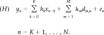 |
The (K + 1)‐dimensional vector h = (h
k)t represents the unknown HRF to be estimated. K is the order of the convolution model, and L = N − K is the actual amount of data used in the calculation. X = (x
n−k) is the regular L‐by‐(K + 1) design matrix, consisting of the lagged stimulus covariates. The L‐by‐M matrix D = (d
m,n) is a basis of M functions that takes a potential drift and any other nuisance effect into account, and the λ = (λm)t are the corresponding coefficients. For the sake of simplicity, the basis is assumed to be orthonormal, i.e.,
 D
t
D = I
L. e = (e
n)t accounts for noise and is supposed to consist of independent and identically distributed Gaussian variables of unknown variance σ2, assumed to be independent from the HRF. As will be shown in the simulation section, this assumption by no way requires that the sampling frequencies of the noise actually corrupting the data be normally distributed. In matrix form, (H) boils down to
D
t
D = I
L. e = (e
n)t accounts for noise and is supposed to consist of independent and identically distributed Gaussian variables of unknown variance σ2, assumed to be independent from the HRF. As will be shown in the simulation section, this assumption by no way requires that the sampling frequencies of the noise actually corrupting the data be normally distributed. In matrix form, (H) boils down to
also called General Linear Model.
Bayesian Analysis With Temporal Prior
What is sought is estimation of the HRF h given the data y. To cope with this issue, a suitable theoretical framework is required for dealing with information coming from various origins. On the one hand, the data follow a known mode, (H). The noise is also supposed to follow a definite (yet general) model, since it is Gaussian. On the other hand, it should be possible to take available information into account, in order to optimize the estimation. The problem faced being ill‐conditioned, a priori knowledge about the HRF needs to be incorporated into the model in order to constrain it and enable coherent estimates. For doing so, Bayesian analysis imposes itself, allowing for robust yet flexible integration of a wide range of information types in a probabilistic framework.
Prior information
Since the underlying physiological process of BOLD fMRI is as of yet only partially understood, setting “hard” constraints on the HRF is most likely to introduce unwanted bias into the estimate. For this reason, we investigate basic and soft constraints that do not contradict current knowledge. More precisely, the following is assumed:
- (P0)
the HRF starts and ends at 0;
- (P1)
the HRF is smooth.
These priors reflect that the underlying process evolves rather slowly on the experimental time scale. Our goal is then to translate this prior knowledge into information that can be directly implemented into a Bayesian analysis. First, prior (P0) can easily be introduced into the model by setting the first and last sample points of the HRF to 0, so that only K − 1 parameters (instead of K + 1) of the HRF are now unknown. Quantification of prior (P1) is achieved by setting a Gaussian prior for the norm of the second derivative of the HRF, whose relative weight is adjusted by a hyperparameter ϵ:
| (1) |
where
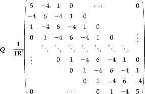 |
is the (K − 1)‐by‐(K − 1) concentration matrix of the Gaussian prior, chosen as the discrete second‐order differentiation matrix. ϵ represents the relative weight of the prior probability compared to the likelihood of the data in the calculation of the posterior probability density function (pdf). The higher ϵ, the more the prior constraint is taken into account. On the contrary, a vanishing ϵ expresses that the solution comparatively integrates much more information from the data. The limiting case ϵ = 0 yields results that are similar to the Maximum‐Likelihood treatment (i.e., Bayesian with no specific prior).
Bayes' Theorem
Once the model and the prior information have been defined, the first step is to use Bayes' theorem stating that, for a set of data compatible with the model:
| (2) |
Since p(y) is independent of h, λ, σ2, and ϵ, it is only a normalization factor that can be discarded from Equation (2), yielding
| (3) |
This equation relates the prior information p(h, λ, σ2, ϵ), the information brought by the data or likelihood p(y|h, λ, σ2, ϵ), and the information inferred a posteriori about the unknown parameters h, λ, σ2 and ϵ, p(h, λ, σ2, ϵ|y). This posterior distribution contains all the knowledge about the parameters that can possibly be inferred from the data and the a priori information we have at hand.
Posterior pdf
Using the chain rule† and assuming no prior dependence between λ, σ2 and ϵ, as well as between h and λ, the prior can be further expanded as
| (4) |
where p(h|σ2, ϵ) has been defined in Equation (1). p(λ), p(σ2), and p(ϵ) are classically set to uninformative priors (flat prior for λ, Jeffreys priors for σ2 and ϵ:
Assuming Gaussian noise, the likelihood rereads
| (5) |
Bringing Equations (4) and (5) together into Equation (3) leads to the posterior pdf for h, λ, σ2 and ϵ:
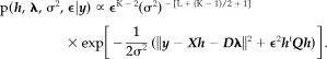 |
(6) |
This distribution is the core of our inference, since any question concerning the problem can be answered by its manipulation and processing.
Marginal posterior pdf for h
In HRF estimation, though, the parameter of interest is usually h. In this case, all other parameters are only nuisance parameters whose estimation is not required, and all information relative to h is contained in the marginal posterior distribution of h, p(h|y). This pdf can in turn be obtained from Equation (6) by integrating it with respect to the other parameters, according to the marginalization formula‡:
Integrating λ and σ2 is straightforward, resulting in
However, this integral cannot be calculated in closed form. A common way to circumvent the problem, as in [Friston et al., 2002a], is to estimate ϵ by  and approximate the sought density by
This approximation holds if p(ϵ|y) is peaked enough around . Practically, checking its validity can be performed by examination of p(ϵ|y) (see, e.g., Fig. 6 for results on real data). p(ϵ|y) can then be approximated by a Dirac function and p(h|y) by
The strategy applied here is to first calculate the posterior pdf for the hyperparameter ϵ as
find an estimator of ϵ and, then, approximate p(h|y) by p(h|y, ϵ = ), which is calculated from the posterior pdf:
An approximation for the marginal posterior for σ2 can also be calculated along the same lines. Using this scheme, it was shown in Marrelec et al. [2001] that
- ϵ follows a pdf that does not belong to any known family, but whose distribution is given by:
where J = I L−(1/L)DD t is the projection matrix estimating and removing the nuisance trend from the data. Numerical calculation of this 1‐dimensional pdf is straightforward, and an estimate can be inferred, such as the Maximum a posteriori (MAP):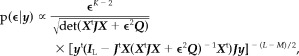
(7)
Choosing the mean instead of the MAP leads to similar results, as shown in Bretthorst [1992].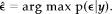
- (σ2|y, ϵ =) is scaled inverse‐chi‐square distributed, with ν = L − M degrees of freedom and scale parameter s
2 = [y
t(I
L − J
t
X(X
t
JX +
2
Q)−1
X
t)Jy]/ν. An estimator of σ2 is given by

(8) - (h|y, ϵ =) is Student‐t distributed with ν degrees of freedom, location parameter
 = (X
t
JX +
2
Q)−1
X
t
Jy and scale matrix V = s
2(X
t
JX +
2
Q)−1. The expectation of (h|y, ϵ = ) can be taken as an estimator for the HRF:
= (X
t
JX +
2
Q)−1
X
t
Jy and scale matrix V = s
2(X
t
JX +
2
Q)−1. The expectation of (h|y, ϵ = ) can be taken as an estimator for the HRF:

(9)
Equation (9) with = 0 corresponds to the well‐known Maximum‐Likelihood estimate (ML estimate) or Ordinary Least Squares estimate (OLS estimate) commonly found in the literature [Mardia et al., 1979; Draper and Smith, 1981]. For ≠ 0, this is the form of a regularized estimator, with playing the role of the regularization parameter. In a typical regularization‐optimization process, one has to minimize a quantity that is the sum of a likelihood function and a regularization/penalization factor (e.g., the norm of the second derivative for smooth variations):
In a Bayesian framework, the value of ϵ can automatically be estimated and set to the most probable value .
Figure 6.
Real data: HRFs (top) and marginal pdfs for ϵ (middle) for each voxel of the clusters shown in Figure 5 (iii). The HRF with highest peak among each region is also represented with standard deviation (bottom). DLPC: dorsolateral prefrontal cortex; CMA: cingulate motor area; lM1: left primary motor area; lPPC: left posterior parietal cortex; rPPC: right posterior parietal cortex.
Divergence Tests on HRFs
Bayesian analysis has recently been applied to activation detection in fMRI data analysis [Friston et al., 2002a,b]. Another approach is to take advantage of the non‐parametric framework developed in this study.
Once the estimation has been carried out as previously explained, it might be of interest to test whether a given function h 0 qualifies as a HRF in a voxel. For instance, if h 0 originates from a biological or physiological model, adequacy of this model with the experimental results can be tested. In a frequentist framework, this corresponds to testing against the null‐hypothesis (h = h 0). In other words, we test whether h is significantly different from h 0. h being Student‐t distributed, the deviance of h 0 from model (H), defined as
should be the realization of a (K − 1) · F K−1,ν‐distributed variable. As proposed in Tanner [1994], we, therefore, define the deviance significance 1 − α0 of (h = h 0) as
| (10) |
where ϕK−1,ν is the cumulative distribution function (cdf) of the F K−1,ν distribution.
An interesting case of hypothesis testing occurs when h 0 is set to 0. The estimated HRF is then compared to a flat function, reflecting a model where the stimulus has no influence on the voxel signal, which is then nothing more than a baseline signal (drift and noise). This is nothing else than activation detection.
In this setting, it is hence possible to estimate the HRF and use the knowledge so gained to perform activation detection on the same dataset. This is possible, since the data are only used once, namely to infer the value of the HRF at each time sample. This information, contained in p(h|y, ϵ = ) and stating that h is t‐distributed with parameters and V, is in turn used to answer questions relative to certain characteristics of the HRF, such as, “What is the shape of the HRF,” or “Is the response function significant?”
RESULTS FROM SYNTHETIC DATA
Materials and Methods
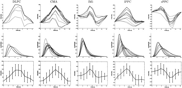
This section deals with the performance of the above estimations and focuses on the three following topics: importance of the temporal prior, relevance of the actual noise sampling distribution and influence of the stimulus sequence. Each feature was analysed using synthetic data. One thousand 224‐point samples were simulated from the same original HRF h 0 (“canonical” HRF used by the SPM99 software§), stimulus sequence (one given realization of a random event‐related stimulus) and quadratic drift as illustrated in Figure 1. Repetition time TR was set to 1.25 sec. The variance of the Gaussian noise σ2 was successively set in {0.001, 0.005, 0.01, 0.05}, corresponding to SNRs¶ given in Table I. For the analysis, K was set to 20 and quadratic drift was considered (M = 3).
Figure 1.
Simulations: (i) HRF h 0, (ii) paradigm, and (iii) quadratic drift.
Table I.
Simulations*
| σ2 | SNR |
|---|---|
| 0.001 | 16.39 |
| 0.005 | 9.40 |
| 0.01 | 6.39 |
| 0.05 | −0.60 |
Noise variances and corresponding SNRs for the HRF defined in Figure 1.
Investigation of HRF estimation performance was assessed using three complementary criteria. First, the quadratic error η1(h) described how close the chosen estimator is to the real HRF. Second, variance score η2(h) was a measure of the uncertainty associated with the given estimator. Now, variance reduction is a desired feature only if the accuracy of the estimator increases consequently. As a matter of fact, a poor estimator (i.e., with high quadratic error) with a low variance is misleading and introduces a bias into the estimation. For instance, introduction of prior information into model (H) has a direct and logical consequence of decreasing the variance of the posterior pdf. By construction, the higher ϵ, the higher the variance reduction. Setting ϵ → ∞ even implies a vanishing variance, |V| → 0, whereas the corresponding estimator tends towards a flat function, which is obviously a very bad estimator of the true HRF. Bias estimation was, therefore, quantified by η3(, V): the smaller the bias, the more conservative the estimate.
Quadratic error was defined in a similar fashion as in Dale [1999]:
| (11) |
It is the average square error per time sample of the estimator compared to the true HRF h 0. Variance score was quantified by
| (12) |
As pointed out in Ruanaidh and Fitzgerald [1996], the determinant of the variance of a distribution has a simple interpretation in terms of hypervolume in a Gaussian approximation. The logarithm of this measure can then be related to an entropic measure.¶ Finally, the bias was measured using the deviance of the real HRF h 0 from the model and Equation (10):
| (13) |
For each series of 1,000 simulations, the corresponding performance estimator was calculated on all the samples.
Importance of the Prior
We first compared a model with no a priori information corresponding to a Maximum‐Likelihood estimation,** called (H L), and the model with the temporal prior, (H B). For typical simulations, Figure 2a represents true and estimated HRFs. Performance estimators were calculated for the 1,000 noise realizations using Equations (11), (12), and (13). The results are summarized in Figures 2b and c.
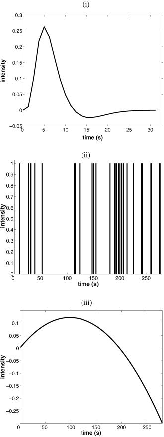
Figure 2.
Simulated data: importance of the prior. a: Typical results of simulations. Top and middle rows: simulated HRF (dotted line) and estimated HRF plus standard deviation (solid line) for the ML estimate (top) and the Bayesian estimate (middle). Bottom row: marginal pdf for ϵ. b: For each noise variance σ2 in {0.001, 0.005, 0.01, 0.05}: (i) relative error of the noise estimator for the ML estimate (light gray) and the Bayesian estimate with prior (dark gray); (ii) relative spread of the estimated ϵ for the model with prior. The mean and the upper and lower 2.5% tails are represented, and the gray area represents the behavior of 95% of the data simulated. c: For each noise variance σ2 in {0.001, 0.005, 0.01, 0.05}: (i) quadratic error η1, (ii) variance score η2, and (iii) deviance significance η3 of the ML estimate (light gray) and the Bayesian estimate with prior (dark gray). The mean and the upper and lower 2.5% tails are represented, and the gray area represents the behavior of 95% of the data simulated.
Figure 2b(i) clearly indicates that, regardless of the noise level, estimates of σ2 were accurate for both models, showing the robustness of this estimator. Figure 2b(ii) shows that the relative spread of in the Bayesian model increased with decreasing SNR. As for HRF estimation, benefits resulting from the introduction of a temporal prior were threefold. First, both models exhibited increasing quadratic error with increasing noise (Figure 2c(i)), but estimator
B (corresponding to model (H
B)) was much more robust to increasing noise than
L (corresponding to model (H
L)). Second, a dramatic decrease of variance was achieved when the prior was considered and, again, the lower the SNR, the larger the difference (Figure 2c(ii)). But this variance reduction was not the source of a bias in the estimation, since the deviance significance of model (H
B) was also improved compared to initial model (H
L), as can be seen on Figure 2c(iii).
Relevance of the Noise Sampling Distribution
According to Bretthorst [1999], the Gaussian structure of the noise in the model is a consequence of the Maximum‐Entropy principle, in which only the mean and the variance of the actual noise are assumed to be known and relevant to the analysis. As such, the estimation should not depend on the sampling frequencies of the noise. This was also observed in Marrelec et al. [2001]. To confirm this, we simulated noise samples from various sampling distributions. First, in accordance with the model hypothesis, Gaussian noise was used with mean 0 and variance 0.01. In order to measure the robustness of the model with regard to the presence of temporal correlation in the noise, AR(4) with exponentially decreasing factors was also simulated.†† Finally, physiological noise was considered as the BOLD fMRI signal of the real data used in the following section, selected in regions where no activation was detected. After every sample, the resulting time series was normed to get the same mean 0 and variance 0.01. Typical results and estimator performances are represented in Figure 3a–c.
Figure 3.
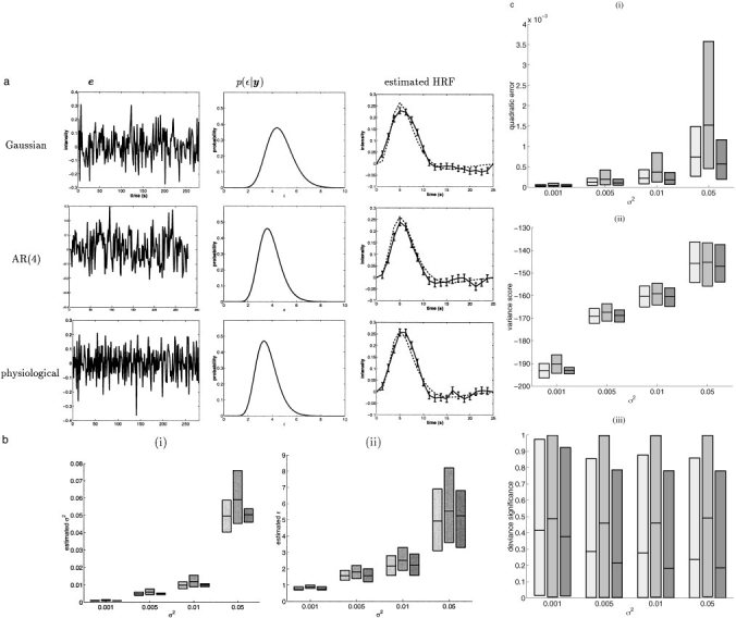
Simulated data: relevance of the noise sampling distribution. a: Typical results of simulations with noise variance σ2 = 0.01 and different noise sampling distributions. Right column: simulated HRF (dotted line) and estimated HRF with standard deviation (solid line). b: For each noise variance σ2 in {0.001, 0.005, 0.01, 0.05} (x‐axis): (i) estimated noise and (ii) ϵ for Gaussian noise (light gray), AR(4) noise (middle gray) and physiological noise (dark gray). c: For each noise variance σ2 in {0.001, 0.005, 0.01, 0.05}: (i) quadratic error, (ii) variance score, and (iii) deviance significance for Gaussian noise (light gray), AR(4) noise (middle gray) and physiological noise (dark gray). The mean and the upper and lower 2.5% tails are represented, and the gray area represents the behavior of 95% of the data simulated.
As evidenced by the results depicted in Figure 3b(ii), estimation of hyperparameter ϵ varied relatively little with respect to the noise distribution: the MAP estimates were consistent with each other. As for the estimate of the noise variance, it was essentially independent from the noise structure (Figure 3b(i)). HRF estimation itself exhibited the same property. From the simulations, it obviously appeared that the actual sampling distribution of the noise is indeed of little importance (Figure 3c(i)–(iii)).
Influence of the Stimulus Sequence
As pointed out in Buxton et al. [2000] and Worsley and Friston [1995], the choice of a stimulus sequence (periodic vs. no‐periodic) is very important and can dramatically influence the power of an estimation method. To demonstrate the behavior of our technique and ensure that the method gives reliable results on the real data (see Results From Real Data), we compared estimates inferred from a simulation with a periodic vs. non‐periodic stimulus. As in the data analyzed in this report, the periodic stimulus repeated itself every 10 s (corresponding to 8 TRs), and we estimated the HRF on 12.5 s (corresponding to K = 10). The results are summarized in Figure 4a–c and must be compared to the results in Figure 2a–c.
Figure 4.
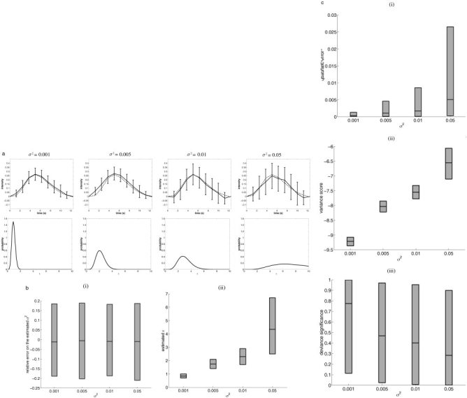
Simulated data: influence of the stimulus. a: Typical results of simulations. Top row: simulated HRF (dotted line) and estimated HRF plus standard deviation (solid line). Bottom row: marginal pdf for ϵ. b: For each noise variance σ2 in {0.001, 0.005, 0.01, 0.05}: (i) relative error of the noise estimator; (ii) estimated ϵ. The mean and the upper and lower 2.5% tails are represented, and the gray area represents the behavior of 95% of the data simulated. c: For each noise variance σ2 in {0.001, 0.005, 0.01, 0.05}: (i) quadratic error η1, (ii) variance score η2, and (iii) deviance significance η3. The mean and the upper and lower 2.5% tails are represented, and the gray area represents the behavior of 95% of the data simulated.
Our first conclusion is that Bayesian analysis is robust with regard to the stimulus sequence. Even though estimates were, as predicted, worse for a periodic stimulus sequence than in the case of non‐periodic stimulus (Fig. 4c vs. Fig. 2c), they did not mislead us, since the variance increased consequently. The resulting bias is comparable to the case where the stimulus is non‐periodic.
RESULTS FROM REAL DATA: VISUO‐SPATIAL JUDGMENT TASK
Materials and Methods
Participants and task
Eleven healthy right‐handed volunteers (age 24–35), with no neurological or psychiatric illness, gave written informed consent and were scanned, while performing the following visual task: they had to decide whether two visual dots flashed on the periphery of an 8‐ray wheel projected on a screen were symmetrical with respect to the central fixation cross. The two dots were presented simultaneously for 150 ms every 10 seconds and their position had to be compared immediately. Subjects had to give a motor response by using a keypad (symmetrical: click with their right index finger; nonsymmetrical: click with their right middle finger). Participants were instructed to maintain eye fixation on the central cross throughout the whole experiment.
Data imaging and preprocessing
A 1.5 Tesla General Electric Signa imager (La Salpêtrière Hospital, Paris) with a standard head coil was used for the imaging. High resolution structural T1‐weighted MPRAGE images were acquired from all participants for anatomical localization (0. 9375 × 0. 9375 × 1.5 mm). The functional images were produced by T2*‐weighted echo‐planar MRI at 8 contiguous 6‐mm axial slices covering dorsal prefrontal and parietal regions (field of view: 24 cm, repetition time TR: 1.25 sec, echo time TE: 60 msec, flip angle: 90 degrees, 64 × 64 matrix of 3.75 × 3.75 mm voxels). Participants were studied in a single 224‐scan session with a total duration of 4 min 40 sec. The scanner was in the acquisition mode for 20 sec before the experiment onset in order to achieve steady‐state transverse magnetization. To compensate for subject motion, images were realigned to the middle image by using a rigid transformation and linear interpolation. The realigned images were filtered for low‐frequency changes in BOLD signal over time by using high‐pass filtering (namely, estimation of the baseline fluctuations using a moving average window and substraction of the estimated baseline from the input signal).
Data Analysis
We estimated the HRF in each voxel. For the analysis, we set the order to K = 10, corresponding to a length of 12.5 sec. We also accounted for quadratic drift (M = 3). To handle significance levels, which were very high, we used the log‐scale: for a significance level 1 − α0, we therefore set q 0 = −log10(1 − α0). We hereafter present the results from one subject.
Activation maps
Using the deviance test proposed in Equation (10), we defined voxel activation as the deviance of the zero HRF function (h 0 = 0) from the model.
The corresponding voxelwise activation map is represented in Figure 5(i). This map can be compared to Figure 5(ii), which was calculated by linear regression from a model with voxelwise adaptive Gaussian functions as proposed by Rajapakse et al. [1998]. It first appears that the two maps are comparable. On the other hand, the significance test developed in this study had a much higher discrimination level compared to the other method. As a matter of fact, regions where there should be no activation (such as the white matter) had a much lower significance in Figure 5(i) than in Figure 5(ii). Moreover, boundaries between activated and not‐activated regions appeared much more clearly and sharply in Figure 5(i) than in Figure 5(ii). Potential activated regions can, therefore, be read off the map with ease. Whether such activated regions are indeed relevant is an issue that cannot be answered here, but high discrimination power is clearly a desired feature.
Figure 5.
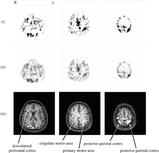
Real data: activation maps. Activation maps from (i) the significance of the divergence test devised in this paper and (ii) the significance test by linear regression on adaptive Gaussian functions. Both maps have the same scale, between 0 (white) and 12 (black); (iii) anatomy and thresholded activation map from (i) (q 0 > 11.5).
Regional stability
The activation map corresponding was thresholded to 1 − α0 = 1 − 10−11.5 (i.e., q 0 = 11.5). From this map, six clusters were selected as shown in Figure 5(iii). For each cluster, Figure 6 represents the HRFs estimated in each voxel of the regions, the corresponding marginals for ϵ as well as the most peaked HRF.
Two main conclusions emerge from there. First, there is a clear idea of intracluster homogeneity. Indeed, the shape of the HRF seemed to be roughly constant within a region, “shape” meaning features of the curve such as increase/decrease, maximum/minimum or time‐to‐peak. However, it is not clear if this similarity is the consequence of physiological homogeneities, since parts of the resemblances may be due to non‐physiological, intrinsic correlation of the signal, originating from the acquisition process or subject movement. On the other hand, the intensity of the response varied greatly in a given region, even though only highly significant voxels were taken into account. Second, HRFs did differ from region to region. They even seemed to be characteristic of the region involved. The differences concern the presence or absence of a post‐stimulus undershoot, the presence or absence of a plateau, the pre‐ and post‐maximum steepness, as well as the time‐to‐peak and the time‐to‐onset.
DISCUSSION
The voxelwise HRF estimation technique that we proposed makes use of basic but relevant a priori information concerning the physiological process underlying the response. It proved to be reliable and robust regarding the actual noise level and structure, as well as the stimulus sequence.
Prior information and bias
Simulations comparing models with and without prior information clearly contradict common belief, which expects that introduction of prior information into analysis necessarily implies an increase of bias. In our case, introduction of a prior actually improved efficiency, variance, and bias at the same time. This is of course true given that the prior knowledge introduced into the model is respected. Estimation of peaked HRFs with this model would certainly give worse results.
Noise structure and estimation
The estimators introduced in this study were shown to be essentially insensitive to the true noise structure. This can be interpretated as follows. Two models were set: one for the HRF, and one for the noise. The latter was based on the sole hypothesis that the noise has given (yet unknown) mean and variance, and the Gaussian structure imposed itself as the least biased under this hypothesis. From there, two situations can happen. If the model for the HRF is sufficiently well defined (i.e., the prior information and the data are sufficient to lead correct inference), then the actual noise structure is mostly irrelevant to the estimation. In this case, introduction of more refined information (e.g., temporal correlation) would only slightly improve the estimation. On the other hand, if the model for the HRF is badly specified, then any additional information will greatly improve the results.
Noise level and smoothness
With decreasing SNR, tends to be set to increasing values, giving more and more importance to the smoothing prior. Slow changes on long scales are then overfavored, and steep variations of the HRF seem to be smoothed out or rounded off (e.g., between 1 and 3 sec and around the peak in the simulations). However, the same simulations showed that our inference is still meaningful, since the mean ± standard deviation estimate stays accurate.
Still with decreasing SNR, p(ϵ|y) becomes more and more diffuse around its peak: the model receives less and less information about the real value of ϵ from the data. Nonetheless, the simulations showed again that the MAP estimator for ϵ still makes sense for our purpose, since the resulting HRF estimates remain accurate. In this case, though, since the variance of ϵ is not considered, it is possible that the variance of h becomes more and more underestimated. This effect could possibly be taken into account (e.g., as proposed by Kaas and Steffey [1989]), at the cost of a more complicated and computationally time‐consuming model. Whether this would significantly improve the inference is not quite clear yet, considered the good behavior of the estimators.
Convolution order
K was not estimated in our analysis but set to a certain value (K = 20 or K = 10). How did the choice of this parameter affect the analysis? Very little, indeed, if the stimulus sequence is of period higher than K or not periodic. In this case, setting K to a value that ensures a small HRF value gives satisfactory results. On the other hand, when the stimulus sequence is periodic, great care has to be taken. Giving K a value higher than the stimulus period implies that the model is not well determined. For this reason, ML estimators cannot be calculated. As we showed, the prior introduced regarding the smoothness of the HRF can somehow make up for this undeterminacy, but there are limits to this. In the simulation example we developed earlier, setting K = 10 is about as far as we could go without getting spurious effects.
CONCLUSION
This report provides an efficient and robust method to estimate the HRF and perform activation detection on the same dataset. The model integrates basic but relevant temporal information about the underlying physiological process of brain activation. Prior knowledge has proven to improve the accuracy and the robustness of the estimators. The actual structure of the noise and its level were shown to have little influence on the performance of the estimation. Simulations also showed that the estimators were robust to the stimulus sequence.
Highly discriminant activation maps were produced from the real data analyzed, as well as a wide variety of HRF shapes. The differences concerned the presence or absence of a post‐stimulus undershoot, the presence or absence of a plateau, the pre‐ and post‐maximum steepness, as well as the time‐to‐peak and the time‐to‐onset. Extra care has, therefore, to be taken when a fixed HRF is chosen and activation detection is performed, since no single function, whatever its characteristics, can account for activation throughout all the brain.
Ongoing research includes the search for new prior information and their translation in terms of constraints. It is also hypothesized that a more general resolution framework (e.g., integration of several stimuli, several sessions) is possible and would greatly improve the estimation.
Acknowledgements
We are thankful to Dr. Stephane Lehéricy (Service de Neuroradiologie, CHU Pitié‐Salpêtrière, Paris), Yves Burnod (INSERM U483, Paris), and Line Garnero (UPR 640 CNRS, Paris) for protocol conception and data acquisition, and to Laura for proofreading the paper. Guillaume Marrelec is supported by the Fondation pour la Recherche Médicale.
Footnotes
p(θ1, θ2) = p(θ1|θ2) · p(θ2).
p(θ1) = ∫ p(θ1, θ2) dθ2.
Defined as SNR =
 ).
).
The entropy of a 𝒩(μ, Σ) distribution is given by S = ½ log[2π exp(1)det(Σ)].
In this case, the order ν changes from K − 1 to K + 1, the number of degrees of freedom changes from L − M to L − M − (K + 1), is set to 0, and all formulas are modified accordingly [Marrelec et al., 2001].
With equation e n = 0. 3679e n−1 + 0. 1353e n−2 + 0. 0498e n−3 + 0. 0183e n−4 + εn and εn ≈ 𝒩(0, 0.01).
REFERENCES
- Aguirre GK, Zarahn E, D'Esposito M (1998): The variability of human BOLD hemodynamic responses. Neuroimage 7: S574. [DOI] [PubMed] [Google Scholar]
- Biswal B, Pathak A, Ward BD, Ulmer JL, Donahue KM, Hudetz AG (2000): Decoupling of the hemodynamic delay from the task‐induced delay in fMRI. Neuroimage 11: S663. [Google Scholar]
- Bretthorst GL (1992): Bayesian interpolation and deconvolution. Tech Rep CR‐RD‐AS‐92‐4. The U. S. Army Missile Command.
- Bretthorst GL (1999): The near‐irrelevance of sampling frequency distributions In: Wolfgang von der Linden, et al., editors. Maximum entropy and Bayesian methods. Dordrecht: Kluwer; p 21–46. [Google Scholar]
- Buckner RL (1998): Event‐related fMRI and the hemodynamic response. Hum Brain Mapp 6: 373–377. [DOI] [PMC free article] [PubMed] [Google Scholar]
- Buckner RL, Koutstaal W, Schacter DL, Dale AM, Rotte M, Rosen BR (1998a): Functional‐anatomic study of episodic retrieval using fMRI (II). Neuroimage 7: 163–175. [DOI] [PubMed] [Google Scholar]
- Buckner RL, Koutstaal W, Schacter DL, Wagner AD, Rosen BR (1998b): Functional‐anatomic study of episodic retrieval using fMRI (I). Neuroimage 7: 151–162. [DOI] [PubMed] [Google Scholar]
- Burock MA, Dale AM (2000): Estimation and detection of event‐related fMRI signals with temporally correlated noise: a statistically efficient and unbiased approach. Hum Brain Mapp 11: 249–260. [DOI] [PMC free article] [PubMed] [Google Scholar]
- Buxton RB, Frank LR (1997): A model for the coupling between cerebral blood flow and oxygen metabolism during neural stimulation. J Cerebr Blood Flow Metab 17: 64–72. [DOI] [PubMed] [Google Scholar]
- Buxton RB, Liu TT, Martinez A, Frank LR, Luh WM, Wong EC (2000): Sorting out event‐related paradigms in fMRI: the distinction between detecting an activation and estimating the hemodynamic response. Neuroimage 11: S457. [Google Scholar]
- Buxton RB, Wong EC, Frank LR (1998): Dynamics of blood flow and oxygenation changes during brain activation: the balloon model. Magn Reson Med 39: 855–864. [DOI] [PubMed] [Google Scholar]
- Chen W, Ogawa S (1999): Principles of BOLD functional MRI In: Moonen C, Bandettini P, editors. Functional MRI. Berlin: Springer; p 103–113. [Google Scholar]
- Dale AM (1999): Optimal experimental design for event‐related fMRI. Hum Brain Mapp 8: 109–114. [DOI] [PMC free article] [PubMed] [Google Scholar]
- Dale AM, Buckner RL (1997): Selective averaging of rapidly presented individual trials using fMRI. Hum Brain Mapp 5: 329–340. [DOI] [PubMed] [Google Scholar]
- Draper N, Smith H (1981): Applied regression analysis. Wiley Series in probability and mathematical statistics, 2nd ed. New York: John Wiley & Sons. [Google Scholar]
- Friston KJ (2002): Bayesian estimation of dynamical systems: an application to fMRI. Neuroimage 16: 513–530. [DOI] [PubMed] [Google Scholar]
- Friston KJ, Jezzard P, Turner R (1994): Analysis of functional MRI time‐series. Hum Brain Mapp 1: 153–171 [Google Scholar]
- Friston KJ, Glaser DE, Henson RNA, Kiebel S, Phillips C, Ashburner J (2002a): Classical and Bayesian inference in neuroimaging: applications. Neuroimage 16: 484–512. [DOI] [PubMed] [Google Scholar]
- Friston KJ, Penny W, Phillips C, Kiebel S, Hinton G, Ashburner J (2002b): Classical and Bayesian inference in neuroimaging: theory. Neuroimage 16: 465–483. [DOI] [PubMed] [Google Scholar]
- Goutte C, Årup Nielsen F, Hansen LK (2000): Modeling the haemodynamic response in fMRI using smooth FIR filters. IEEE Trans Med Imag 19: 1188–1201. [DOI] [PubMed] [Google Scholar]
- Gössl C, Auer D, Fahrmeir L (2001a): Bayesian spatiotemporal inference in functional magnetic resonance imaging. Biometrics 57: 554–562. [DOI] [PubMed] [Google Scholar]
- Gössl C, Fahrmeir L, Auer DP (2001b): Bayesian modeling of the hemodynamic response function in BOLD fMRI. Neuroimage 14: 140–148. [DOI] [PubMed] [Google Scholar]
- Kaas RE, Steffey D (1989): Approximate Bayesian inference in conditionally independent hierarchical models (parametric empirical Bayes models). J Am Stat Assoc 84: 717–726. [Google Scholar]
- Kershaw J, Abe S, Kashikura K, Zhang X, Kanno I (2000): A Bayesian approach to estimating the haemodynamic response function in event‐related fMRI. Neuroimage 11: S474. [Google Scholar]
- Kruggel F, von Cramon DY (1999a): Modeling the hemodynamic response in single‐trial functional MRI experiments. Magn Reson Med 42: 787–797. [DOI] [PubMed] [Google Scholar]
- Kruggel F, von Cramon DY (1999b): Temporal properties of the hemodynamic response in functional MRI. Hum Brain Mapp 8: 259–271. [DOI] [PMC free article] [PubMed] [Google Scholar]
- Kruggel F, Zysset S, von Cramon DY (2000): Nonlinear regression of functional MRI data: an item recognition task study. Neuroimage 12: 173–183. [DOI] [PubMed] [Google Scholar]
- Li TQ, Haefelin TN, Chan B, Kastrup A, Jonsson T, Glover GH, Moseley ME (2000): Assessment of hemodynamic response during focal neural activity in human using bolus tracking, arterial spin labeling and BOLD techniques. Neuroimage 12: 442–451. [DOI] [PubMed] [Google Scholar]
- Logothetis NK, Pauls J, Augath M, Trinath T, Oeltermann A (2001): Neurophysiological investigation of the basis of the fMRI signal. Nature 412: 150–157. [DOI] [PubMed] [Google Scholar]
- Mardia KV, Kent JT, Bibby JM (1979): Multivariate analysis. Probability and mathematical statistics. London: Academic Press. [Google Scholar]
- Marrelec G, Benali H (2001): Non‐parametric Bayesian deconvolution of fMRI hemodynamic response function using smoothing prior. Neuroimage 13: S194. [Google Scholar]
- Marrelec G, Benali H, Ciuciu P, Poline JB (2001): Bayesian estimation of the hemodynamic response function in functional MRI In: Fry R, editor. Bayesian inference and maximum entropy methods in science and engineering: 21st International Workshop. Melville: AIP; p 229–247. [Google Scholar]
- Miezin FM, Maccotta L, Ollinger JM, Petersen SE, Buckner RL (2000): Characterizing the hemodynamic response: effects of presentation rate, sampling procedure, and the possibility of ordering brain activity based on relative timing. Neuroimage 11: 735–759. [DOI] [PubMed] [Google Scholar]
- Rajapakse JC, Kruggel F, Maisog JM, von Cramon DY (1998): Modeling hemodynamic response for analysis of functional MRI time‐series. Hum Brain Mapp 6: 283–300. [DOI] [PMC free article] [PubMed] [Google Scholar]
- Ruanaidh JJKO, Fitzgerald WJ (1996): Numerical Bayesian methods applied to signal processing. Statistics and computing. New York: Springer. [Google Scholar]
- Tanner MA (1994): Tools for statistical inference: methods for the exploration of posterior distributions and likelihood functions. Springer Series in statistics, 2nd ed. New York: Springer. [Google Scholar]
- Vazquez AL, Noll DC (1996): Non‐linear temporal aspects of the BOLD response in fMRI. Proc ISMRM 1st Annual Meeting. p 1765.
- Worsley KJ, Friston KJ (1995): Analysis of fMRI time‐series revisited‐again. Neuroimage 2: 173–181. [DOI] [PubMed] [Google Scholar]