Recursive penalized least squares solution for dynamical inverse problems of EEG generation

Abstract

In the dynamical inverse problem of electroencephalogram (EEG) generation where a specific dynamics for the electrical current distribution is assumed, we can impose general spatiotemporal constraints onto the solution by casting the problem into a state space representation and assuming a specific class of parametric models for the dynamics. The Akaike Bayesian Information Criterion (ABIC), which is based on the Type II likelihood, was used to estimate the parameters and evaluate the model. In addition, dynamic low‐resolution brain electromagnetic tomography (LORETA), a new approach for estimating the current distribution is introduced. A recursive penalized least squares (RPLS) step forms the main element of our implementation. To obtain improved inverse solutions, dynamic LORETA exploits both spatial and temporal information, whereas LORETA uses only spatial information. A considerable improvement in performance compared to LORETA was found when dynamic LORETA was applied to simulated EEG data, and the new method was applied also to clinical EEG data. Hum. Brain Mapp. 21:221–235, 2004. © 2004 Wiley‐Liss, Inc.

INTRODUCTION

Measurements of electromagnetic fields on the scalp surface provide valuable information about underlying brain dynamics. Electroencephalograms (EEGs) are obtained by measuring the electrical potential on several scalp surface locations. It is commonly believed that these potentials are generated by electrical currents in the extracellular media, resulting from electrical and chemical activity of neurons.

There is considerable interest in noninvasive localization of electrical generators in the brain. The attempt to estimate these generators, based on EEG measurements, is an example of an inverse problem. The main difficulty in solving this inverse problem arises from the fact that the EEG observations do not contain sufficient information to precisely reproduce these generators. For this reason, the solution of the inverse problem (i.e., the inverse solution) will be non‐unique, because a given set of EEG measurements will have an infinite number of possible inverse solutions consistent with the measurements. Additional physiological or physical information about the generators is needed to identify a unique solution.

A common approach to the EEG inverse problem is to assume a distributed source model, which employs discretization of brain volume into a set of voxels, each of which is considered to be the location of a current vector. To obtain a unique solution, various constraints have been suggested previously, such as optimal resolution [Backus and Gilbert, 1968; Grave de Peralta Menendez et al., 1997; Grave de Peralta Menendez and Gonzalez Andino, 1999], L2 minimum norm [Hämäläinen and Ilmoniemi, 1984], L1 minimum norm (called selective minimum norm) [Matsuura and Okabe, 1995], and maximum spatial smoothness, called low resolution brain electromagnetic tomography (LORETA) [Pascual‐Marqui et al., 1994].

Relative advantages and disadvantages of these approaches have been discussed previously from a purely spatial point of view [Grave de Peralta Menendez and Gonzalez Andino, 2002; Pascual‐Marqui, 1999; Pascual‐Marqui and Michel, 1994]. These approaches exclusively use the information from one instantaneous measurement, i.e., the set of voltage measurements obtained from various electrodes at one single instant of time, whereas EEG measurements clearly have temporal structure.

Recently, temporal constraints have been considered for various applications related to inverse problems. In the analysis of electrocardiograms (ECG), an algorithm has been proposed for solving large‐scale least squares problems based on multiple constraints, including explicit spatial and temporal constraints [Brooks et al., 1999]. For current distribution reconstruction in the EEG inverse problem, or more generally in the EEG/magnetoencephalography (MEG) inverse problem, other algorithms have been developed for solving the above‐mentioned large‐scale least squares problem [Schmitt et al., 2001; Schmitt and Louis, 2002a, b]. Inverse problems arising in analysis of data obtained by electrical impedance tomography (EIT) and single photon emission tomography (SPET) have been formulated as state estimation problems [Kaipio et al., 1999; Karjalainen et al., 1997; Vauhkonen et al., 2001]; the use of Kalman filtering and Kalman smoothing has been suggested for obtaining estimates of the state. The introduction of a temporal constraint into the EEG/MEG inverse problem by employing a time window and Gaussian kernels has been suggested by Phillips et al. [2002].

Temporal constraints, as used previously, refer only to the aspect of temporal smoothness. We consider a more general variant of temporal constraints by regarding time‐dependent EEG measurements as reflecting generators that evolve according to some dynamics, a problem called the dynamical inverse problem. It will be possible to express explicitly the spatiotemporal constraints as part of the system equation within the state space representation by formulating the dynamical inverse problem of EEG generation as a state estimation problem. In particular we emphasize the application of the established procedures of statistical modelling: they require us to assume a class of parametric models and to compare these models using likelihood as a criterion.

In principle, state estimation and model comparison could be implemented using Kalman filtering. Due to the high dimensionality of state (corresponding to the high voxel number), however, the direct application of conventional Kalman filtering to the EEG inverse problem is impracticable. We introduce a simple and computationally efficient estimation procedure based on the recursive penalized least squares (RPLS) method. In addition, we employ the Akaike Bayesian Information Criterion (ABIC) [Akaike, 1980a, b] as a statistical criterion for estimating the regularization parameter and for comparing models. As a result, we obtain dynamic low‐resolution brain electromagnetic tomography (DynLORETA), a new algorithm for estimating inverse solutions from EEG time series. DynLORETA combines the spatial smoothness constraint of the LORETA method with additional dynamical constraints.

After a brief review of the forward problem of EEG generation, the dynamical inverse problem, as compared to the instantaneous inverse problem, is introduced. Then we review LORETA and introduce DynLORETA; as a simple approach to the estimation of generators the RPLS method is proposed. A simulation study is used to compare DynLORETA with (instantaneous) LORETA and the DynLORETA method is applied also to clinical EEG data.

The following notation is used throughout this article: the transpose of a matrix A is denoted by A′, and a n × n identity matrix is denoted by I _n. For a vector x and a positive definite matrix C, we define ∥x∥_C = x′C ⁻¹ x. The L2 norm of a vector x is denoted by ∥x∥, corresponding to the case of C being an identity matrix.

Forward Problem

The relationship between scalp surface EEG measurements and the primary current density resulting from neuronal activity is described by the equation

(1)

In equation (1), Y denotes a vector of length d that contains the EEG measurements of scalp electric potential differences at d electrodes. J = (j′₁, … j′ ${}_{\mathit{\text{N}}{}_{\mathit{\text{j}}}}$)′ denotes a vector of length D = 3N _j, which contains the current density vectors j _v = (j _xv, j _yv, j _zv),(v = 1, …, N_j) at N _j voxels in the brain. The matrix K, linking the current density J with the measurement Y, is called the lead field matrix. It can be calculated by applying Maxwell's equations to a particular head model [Nunez, 1981]. The vector ϵ is an additive random element representing unmodeled effects such as observation noise. The forward problem consists of calculating the measurement Y from given current density J.

Inverse Problem

The inverse problem is defined the estimation of current density J from given measurement Y and constitutes an ill‐posed problem, because the number of scalp electrodes is much smaller than the number of voxels for which the current density has to be estimated. We therefore need to impose additional constraints as prior knowledge. In particular, we call the inverse problem, as formulated by equation (1), the instantaneous inverse problem, because only the measurement at one single time point is used to estimate J.

The definition of dynamic(al) inverse problems was first discussed explicitly by Schmitt and Louis [2002a]. They defined the instantaneous (static) inverse problem as follows: “The properties J of the examined object do not change during the measuring process. Thus, we have to solve K J = Y _i for all i.” On the other hand, they defined the dynamical inverse problem as follows: “The examined object is allowed to change during the measuring process and we have to solve KJ _i = Y _i for all i.” Because the term “dynamical inverse problem” was used to describe broadly any time‐varying situation, without reference to particular variations in time resulting from an actual dynamical evolution, the term “nonstationary inverse problem” may seem more suitable for their definition.

We use the term “dynamical inverse problem” for a slightly more restricted situation, which is defined as follows: “Solutions of a dynamical inverse problem have to be in agreement with a twofold set of restricting information, represented by the observation equation for all time points considered, Y _t = KJ _t + ε_t (t = 1, 2,…), and by some prespecified dynamics about J _t, J _t−1, J _t−2, ….” On the other hand, we define the “instantaneous inverse problem” as follows: “Solutions of an instantaneous inverse problem have to be in agreement with a twofold set of restricting information, represented by the observation equation at one fixed time point Y = KJ + ε, and prior knowledge about J.” In our definition, we impose an explicit assumption for the time course evolution of J _t to simplify the mathematical formulation of the problem.

In the instantaneous inverse problem, the solution reflects only an instantaneous observation Y _t, whereas in the dynamical inverse problem it reflects a sequence of temporally successive observations Y _t, Y _t−1 ⋮ such that some dynamics of the generator are imposed. As shown in Figure 1, the dependence of Y _t on the evolution of J _t is considered explicitly in the dynamical inverse problem. If J _t evolution does not follow any dynamics, the dynamical inverse problem becomes equivalent to the instantaneous problem, i.e., becomes a generalization of the instantaneous problem.

Figure 1.

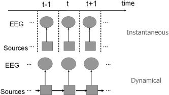
Schematic comparison between the instantaneous inverse problem (top) and the dynamical inverse problem (bottom). Sources within brain and EEG observations represented by rectangles and circles, respectively. Arrows represent the flow of information, as assumed by the underlying model.

MATERIALS AND METHODS

LORETA

LORETA was suggested first by Pascual‐Marqui et al. [1994] to overcome the inability of previous approaches to correctly localize the 3‐D solution spaces. As prior knowledge, LORETA imposes a spatial smoothness constraint onto the solution J. This spatial smoothness constraint is expressed using the (3‐D discretized) Laplacian matrix L

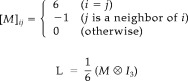The ith row vector of L acts as a discrete differentiating operator by forming differences between the nearest neighbors of the ith voxel and ith voxel itself.

The solution of LORETA is obtained by minimizing a linear mixture of a weighted norm ∥LJ∥ and the residuals of the fit according to the observation equation. By assuming a Gaussian distribution ϵ ∼ N(0, σ² C _ϵ) with known covariance structure C _ϵ for the measurement noise in equation (1), the objective function of LORETA becomes

(2)

where the parameter λ, called the regularization parameter, expresses the balance between fitting the model and the prior constraint of minimizing ∥LJ∥. The solution of this minimization problem for a given λ is obtained by

Dynamical LORETA

Dynamical constraint

Pioneering work on obtaining dynamical inverse solutions with spatial and temporal smoothness constraints has been presented by Schmitt et al. [2001] for the EEG inverse problem. They formulated the spatial smoothness constraint by using the Laplacian operator and the temporal smoothness constraint by using a time‐domain differencing operator. Their temporal smoothness constraint can be interpreted as assuming a random walk model J _t = J _t−1 + η_t for the dynamics of J _t. In addition to the spatial smoothness constraint, a more general class of dynamical constraints is employed for DynLORETA.

Similar to that introduced in Schmitt et al. [2001], an objective function containing the spatial and temporal smoothness constraints is defined:

(3)

Interactions between neighboring voxels can also be taken into account by including the Laplacian matrix L into the third term of equation (3), and this step considerably reduces the computational expenses.

By introducing a new parameter ϕ that represents a balance between the second and third terms of equation (3), we can combine the two penalty terms and obtain a more compact expression:

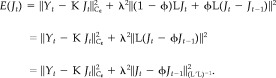(4)

The objective function equations (3) and (4) are not equivalent mathematically; however, equation (4) can be regarded as a different way of imposing these two kinds of constraints.

To rewrite this objective function in the form of a statistical model, from equation (4) we obtain the state space representation given by

(5)

(6)

Equations (5) and (6) represent the observation equation and the system equation, corresponding to the first and second term of equation (4), respectively. An important advantage of state space representations is that a more general dynamical model can be designed by changing the system equation. For example, a more complex dynamical model can be considered that also includes previous states beyond the first lag and allows for interactions between generators on different voxels:

(7)

where A _i (i = 1, …, p) are D×D matrices. Whereas equation (6) represents the case of very simple dynamics, various interesting dynamics can be modeled by equation (7), displaying features such as spatial heterogeneity, local neighbor interaction, etc.

The state space representation with very general dynamics in the system equation is given by:

(8)

where S denotes exogenous variables and can model some external force influencing the brain. The function f _t( ·) may be specified as linear, as in the case of equation (7), or may be taken as nonlinear or time‐dependent.

Three key points should be emphasized. First, the covariance structure of the system noise η_t should be given by (L′L)⁻¹. It is expected that spatial smoothness of J _t will be inherited from instantaneous LORETA. Second, as stated already, the model is written in a state space representation. In principle, it is possible to carry out optimal inference about J _t by employing the Kalman filter or the extended Kalman filter [Aoki, 1987; Durbin and Koopman, 2001; Jazwinski, 1970; Kitagawa and Gersh, 1996]. Third, the kind of dynamics assumed depends on the analyst. Because there are many possible solutions corresponding to different dynamical models, the resulting solutions should be evaluated by some statistical criterion, such as ABIC.

Approximate estimation

As mentioned above, in principle, we could obtain the estimate of J _t(t=1, …, T) using Kalman filtering. In the least squares case, the filtered estimator J _t|t(t=1, …, T) obtained by Kalman filtering is the best possible estimator based on past and current observations. In the 3‐D discretized inverse problem, however, the dimension D of the state J _t is three times the number of voxels (typically several thousand). The practical application of Kalman filtering to such a very high‐dimensional state vector would therefore be very demanding (or even impossible) in terms of computational time and memory consumption (e.g., due to the need to compute and store dense matrices of size D×D). To overcome this difficulty, it is necessary to design suitable approximations of the standard Kalman filtering approach. Galka et al. [2002] presented a new approach to spatiotemporal Kalman filtering that renders this high‐dimensional filtering problem tractable. In the present work, we introduce a different, very simple estimation procedure that requires only minor modification of instantaneous LORETA. This procedure is termed the recursive penalized least squares (RPLS) solution.

For notational simplicity, we assume that the function f _t(·) in equation (8) is linear and depends only on the states of the generators at the previous time step:

(9)

where A _t denotes a known matrix of size D×D. The assumption of linearity, however, is not essential for the RPLS solution. The practical estimation procedure is discussed in detail below.

An initial estimate (for t = 1) of the state J ₁ can be obtained by any approach for solving the instantaneous inverse problem. For t = 2,3, …, T, we can obtain an estimate of J _t by recursively solving the penalized least squares problem

(10)

where _t−1 is the estimate obtained in the previous step. The solution of equation (10) is given by

(11)

Direct computation of this expression is numerically impracticable, however, because a large matrix of size D×D needs to be inverted; here, D is the dimension of the state. By appropriate variable transformation, a numerically more easily accessible solution may be obtained. In addition, this transformation clearly demonstrates the relationship between the RPLS method and Kalman filtering (see Appendix A).

We start from the following variable transformations:

(12)

(13)

where ς_t and r _t correspond to system noise and innovation (1‐step ahead prediction error), respectively. The objective function of equation (10) can be rewritten as follows:

(14)

An estimate of J _t can then be obtained by

(15)

(16)

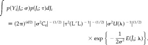
where we have defined

(17)

(18)

Here, U, diag(s_i), V are d × d, d × d and D × d matrices obtained from the singular value decomposition (SVD) of C _ε ^−1/2KL⁻¹ [Mardia et al., 1979]. Computation of equation (18) is not as demanding as the computation of equation (11), because in equation (18) the large matrix to be inverted does not depend on λ, such that this inversion needs only to be carried out once, whereas in equation (11) the inversion has to be carried out repeatedly during the process of finding an optimal λ value. A similar remark applies to the SVD of C _ε ^−1/2KL⁻¹ that also needs to be computed only once, because these three matrices are known.

Estimating regularization parameter λ

The regularization parameter λ should be chosen in an objective way, because the inverse solution will depend sensitively on this parameter. Various methods, such as the generalized cross‐validation (GCV) criterion [Wahba, 1990] and the L‐curve method [Hansen, 1992, 1994] have been employed for choosing the regulation parameter. In the present work, we propose to employ ABIC [Akaike, 1980a, b] for estimating this parameter, because this criterion can be applied not only for selecting the regularization parameter, but also for the purpose of model comparison.

ABIC is defined as

where N is the number of hyperparameters in the model and l ^(II) (σ,τ) is the likelihood of the hyperparameters in the context of empirical Bayesian inference, called Type II log‐likelihood. If there are unobservable variables in the model, the Type II likelihood can be obtained by averaging the joint distribution of all variables, both observable and unobservable, over the unobservable variables:

(19)

where Y _t are the observable and J _t the unobservable variables, σ and τ are hyperparameters.

It is very difficult to calculate analytically this multiple integral for the dynamical inverse problem. Equation (19) can therefore be approximated by the sum of Type II log‐likelihoods at each time point, l ^(II) (σ, τ). Because the inference (if interpreted from the Bayesian viewpoint) in the RPLS method is based on p(r _t |ς _t ; σ) and p(ς _t ; τ) as likelihood and prior distribution, respectively (compare equations [12] and [13]), the pointwise Type II log‐likelihood based on r _t is given by

(20)

Then l ^(II)(σ, τ) is approximated by the summation of l ${}_{\text{t}}^{\text{(II)}}$(σ, τ). This approximation is justified if the innovations r _t (t = 1, …, T) are serially independent with respect to their distributions p(r _t).

If p(r _t |ς _t; σ) and p(ς_t; τ) are assumed to be Gaussian, we can analytically calculate this integral and obtain (−2) times the pointwise Type II log‐likelihood:

(21)

where _i,j is the ith component of the vector U′C ${}_{\text{ε}}^{\text{−1/2}}$ r _t (see Appendix B for detail). Here, the hyperparameter τ was been replaced by λ = σ/τ. A constant term has been ignored in equation (21). ABIC can then be expressed by

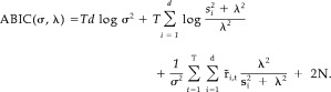(22)

Estimates of and can be obtained by minimizing this expression, and the resulting minimum value of ABIC can be employed for model comparison.

If a parametric model of the dynamics is assumed, this model will contain unknown parameters θ, which have to be estimated. This can be done by minimizing ABIC, as given by equation (22), but the innovations (1‐step prediction errors) r _t now depend on these parameters, such that ABIC(σ, λ) becomes ABIC(σ, λ, θ). In our implementation, this optimization is carried out by the simplex method, as provided by the “fminsearch” function of Matlab.

RESULTS

For the calculations in the simulation study and analysis of real EEG data, the following practical settings were chosen: the lead field matrix K was calculated with a three‐shell head model [Riera and Fuentes, 1998]; a brain model derived from the average probabilistic magnetic resonance imaging (MRI) atlas produced by the Montreal Neurological Institute [Mazziotta et al. 1995] was employed; and the voxel discretization resolution was 7 mm, resulting in a total of 8,723 voxels. Generators were assumed to be located only within gray matter, reducing to 3,433 the number of voxels considered. The number and locations of EEG electrodes followed the standard 10‐20 system.

Simulation Example

To compare inverse solutions obtained by LORETA and DynLORETA, a simulation experiment was carried out. We generated a time series of T = 300 observations from a AR(2) model of voxel dynamics, including nearest‐neighbor interactions, as describe by

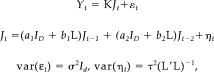where the parameters were chosen as (a ₁, a ₂, b ₁, b ₂, σ, τ) = (1.82, −1.00, 0.05, 0.00, 0.03, 0.01), and the vectors of initial current densities J ₀, J ₋₁were chosen so that two extended sources of activity were created, one in the occipital region and one in the cingulate gyrus. Figure 2 shows the EEG observations Y ₁, …, Y _T corresponding to the simulated J₁, …, J _T with respect to right‐ear mastoid reference. A stationary oscillation can be seen at most electrodes, except those located within the frontal region. A spatial representation of J ₀ is shown in Figure 3 (top left).

Figure 2.

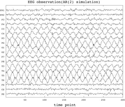
Simulated EEG observations at 19 standard electrode positions of the 10/20‐system vs. simulation time, according to the simulation example described in the text.

Figure 3.

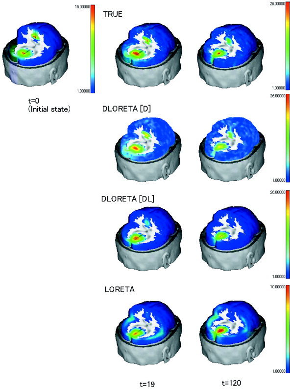
Spatial distributions of absolute values of local current vectors for the simulation (TRUE) and for the inverse solutions obtained by DynLORETA with known initial state [D], by DynLORETA with unknown initial state [DL], and by LORETA [L]. Top left: Initial state of the simulation. Middle, right: Inverse solutions at time points t = 19 and t = 120, respectively. Note that color scale of [L] is different from the color scale of the other three rows.

From these observations, estimates of sources were calculated using the following three methods and conditions: DynLORETA with unknown dynamical parameters and known true initial current vectors (denoted by [D]); DynLORETA with unknown dynamical parameter and initial current vectors based on LORETA inverse solutions (denoted by [DL]); and instantaneous LORETA (denoted by [L]).

For each method, both ABIC and GCV were used to estimate the regularization parameter λ, and dynamical parameters of methods [D] and [DL] were estimated by minimizing equation (22). The resulting estimates and the corresponding values of ABIC and GCV are shown in Table I. The results displayed in the table demonstrate that estimating λ using the ABIC criterion is as good as using the computationally more intensive GCV approach.

Table I.

Estimates of regularization parameter λ and dynamical parameters, and corresponding values of ABIC and GCV for the simulation data

	DynLORETA [D]	DynLORETA [DL]	LORETA [L]
λ GCV	0.256	0.095	0.0076
λ ABIC	0.259	0.100	0.0065
GCV	2.58 × 10−6	2.69 × 10−6	3.71 × 10−6
ABIC	−4.18 × 104	−3.95 × 104	−3.56 × 104
( 1, 2, 1, 2)	(1.82, −1.00, 0.06, 0.008)	(1.87, −1.05, −0.57, 0.58)	·

These values are obtained by DynLORETA with known initial states [D], DynLORETA with estimated initial states [DL], and LORETA [L].

In Figure 3, we show for time points t = 19 and t = 120 the spatial distributions of absolute values of local current vectors for the simulation (“truth”) and for inverse solutions obtained by [D], [DL], and [L]. It can be seen that [D], [DL] and [L] successfully reproduced the occipital activity source, although [L] considerably underestimated the amplitude at the center of this source. In addition, [L] completely failed to reproduce the independent source in the cingulate gyrus, which was well reconstructed by [D]. [L] instead produced spurious activity in the temporal region. For t = 120, [DL] also failed to reproduce the source in the cingulate gyrus, which reflected the rapid decay of the estimated dynamics (compare the corresponding subfigure in Fig. 4).

Figure 4.

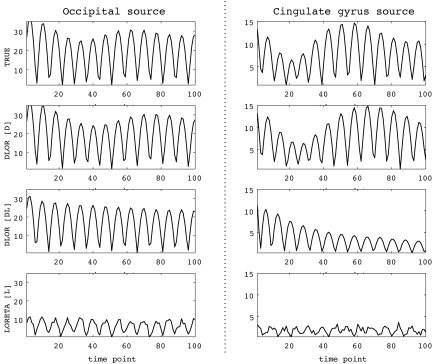
Time series of absolute values of local current vectors at two individual voxels, one from occipital area (left) and one from cingulate gyrus (right), vs. simulation time. Top to bottom rows: Simulated time series and results for inverse solutions obtained by DynLORETA with known initial state [D], DynLORETA with unknown initial state [DL], and by LORETA [L].

In Figure 4, the same results are presented for the time domain. For two specific voxels chosen from the occipital area and the cingulate gyrus, the corresponding time series are shown for absolute values of current vectors for simulation and inverse solutions obtained by [D], [DL], and [L]. It can be seen that the solution with [D] coincided very well with the simulated time series for both voxels; this success was due to accurate dynamical parameter estimates (see Table I). With respect to the main oscillation, [DL] reproduced qualitatively the behavior of the simulated time series for both voxels. Deviations from the simulated time series increased with time, however, reflecting the use of inaccurate dynamical parameter estimates. Although to some extent [L] also reproduced oscillations for both voxels, this solution completely failed to reproduce their amplitudes correctly. Furthermore, [L] lacked temporal smoothness, a consequence of the incapability of LORETA to discriminate between dynamical and observation noise, a weakness of instantaneous inverse solutions noted previously by Schmitt et al. [2001].

The goodness of solutions obtained by the three methods can be compared. As can be seen in Table I, there is a succession of [D], [DL] and [L] with respect to increasing values of ABIC. From the viewpoint of model comparison, this result shows that solution of [D] was better than that of [DL], which was better than that of [L]. ABIC, however, is of value only as a relative measure. The difference between the ABIC values of two models has the interpretation of a ratio of probabilities, but the values themselves have no meaningful interpretation.

Compared to [L], [DL] provides considerably better inverse solutions, even though there remained an underestimation of the amplitudes from true sources, resulting from inaccurate initial state estimates and consequently inaccurate estimated dynamics. This is an important result, because in contrast to [D], [DL] is applicable to the analysis of real data. The superior results obtained by [D], however, indicate that further improvements can be achieved in future work by adjusting the estimation procedure for the initial state.

Real Data Analysis

A clinical EEG recording recorded from a healthy child in awake state with closed eyes is shown in Figure 5. An oscillation representing the characteristic α rhythm is visible at occipital electrodes O1 and O2. For analysis of this data set, a regional homogeneous AR(2) model is employed, given by

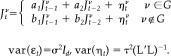Figure 5.

Clinical EEG recording at 19 standard positions of the 10/20‐system vs. time (obtained from a healthy 8‐year‐old male child awake with eyes closed). Vertical axis represents observed voltages relative to the average reference.

The dynamics within a certain region G is assumed to differ from the dynamics within the remaining part of brain. We have chosen the region G as a sphere of radius 30 mm centered within the occipital lobes; the center was chosen according to a LORETA solution of the same data.

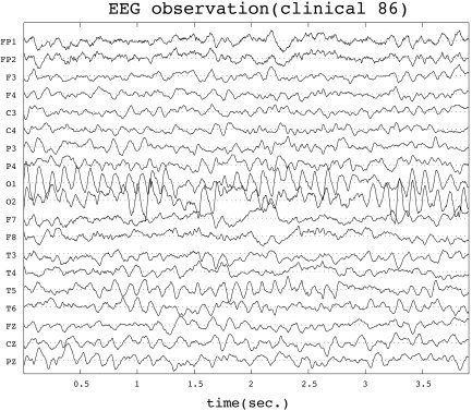
In Figure 6, the time series and periodograms of the x,y,z components of the current vector from a particular voxel inside G are shown. In each figure, the time series and periodograms estimated by both LORETA and DynLORETA are plotted. Each component of the time series provided by DynLORETA shows clearer α oscillations compared to that in the LORETA time series. In the periodograms, this difference can also be seen in the range of the α rhythm (around 9 Hz). In addition, the time series provided by DynLORETA have higher amplitude than do the time series provided by LORETA; this effect had also been shown in the previous simulation experiment.

Figure 6.

Time series of the x, y, z components of estimated local current vector at one voxel, chosen from G (occipital area) (top) and corresponding periodograms (bottom) for inverse solutions obtained from EEG data set from Figure 5. Thin lines, DynLORETA; thick lines, LORETA.

Estimation of the dynamical parameters (a ₁, a ₂, b ₁, b ₂) by numerical optimization provides the estimates (1.95, −0.99, 1.54, −0.56). The parametric power spectrum [Shumway, 2000], as obtained from the estimated AR parameters inside G displays a peak around 8.3 Hz, whereas the power spectrum outside G does not display a peak, just a drop in power toward higher frequencies. The peak at 8.3 Hz falls well within the known range for α activity. These results illustrate that by DynLORETA, it is possible to make detailed inferences about the dynamics of generators of EEG time series.

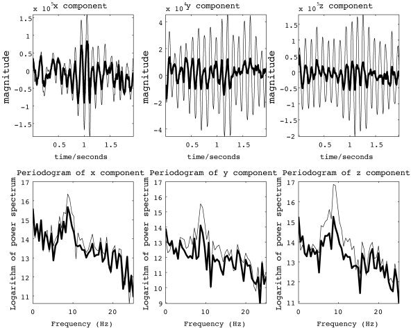
In Figure 7, evolution of spatial distribution of a current vector component, as estimated by DynLORETA and LORETA, is illustrated for six consecutive points of time (with a time shift of 0.0234 sec). The figure displays the current vector component that corresponds to the radial direction of spherical coordinates, with the origin at the center of the head. DynLORETA and LORETA solutions both provide two main sources that are negatively correlated in the left and right occipital region. These two sources can be considered generators of α rhythm [Rodin and Rodin, 1995; Valdés‐Sosa et al., 1992]. The solution obtained by DynLORETA shows much more focused sources in the occipital region, however, whereas the LORETA solution shows spurious activities in other regions, such as the temporal lobes and around the vertex (electrode Cz). In addition, the quality of the inverse solutions provided by LORETA and DynLORETA can be assessed by comparing their corresponding values of ABIC, which are 1.76 × 10⁵ and 1.24 × 10⁵, respectively. Comparison of these ABIC values proves that the solution provided by DynLORETA is superior to that provided by LORETA.

Figure 7.

Spatial distributions of current vector component corresponding to radial direction of spherical coordinates for inverse solutions obtained from EEG data set in Figure 5. Top: Solutions estimated by DynLORETA; bottom: solutions estimated by LORETA (both at 6 consecutive points in time).

DISCUSSION

We have addressed the inverse problem of estimating generators of EEG recordings, with particular emphasis on the use of dynamical constraints, i.e., the dynamical inverse problem of EEG generation. We studied the dynamical inverse problem of EEG generation. By formulating the dynamical inverse problem in a state space representation, we can introduce general dynamical constraints into the system equation.

In principle, the optimum solution of this state estimation problem is given by Kalman filtering and Kalman smoothing; however, due to the high dimensionality of state in the EEG inverse problem, direct application of Kalman filtering is very demanding (or even impossible) in terms of computational time and memory consumption. As an alternative, we employed the RPLS method. The relationship between the RPLS method and Kalman filtering is discussed in detail in Appendix A.

As a practicable approach for finding solutions of the dynamical inverse problem for given data without excessive computational expense, we introduced a suitable method, which we have called dynamical LORETA (DynLORETA), because it is derived from the LORETA method for solving the instantaneous problem. It is a crucial advantage of DynLORETA that by suitable choice of the system noise covariance structure it inherits from LORETA the desirable feature of maximum spatial smoothness.

On a PC with a clock rate of 2 GHz, the computation of DynLORETA for an EEG data set consisting of 500 time points takes a few hours, including optimization of several hyperparameters. In contrast, for the same data set, the computation of LORETA takes only a few seconds, including optimization of the regularization parameter. This difference results from the higher number of hyperparameters to be optimized in DynLORETA and the need to compute for each time point t several additional multiplications and summations of high‐dimensional matrices within the state space framework. To obtain inverse solutions of improved quality, such a price in terms of high computational expense has to be paid.

We have proposed the use of ABIC to estimating hyperparameters, especially the regularization parameter. It was found in a simulation study that ABIC and GCV criteria provide similar estimates. ABIC is valuable for model comparison, because it can be interpreted as the goodness of fit of the model to the data. ABIC is a relative measure, and although the value of ABIC itself has no meaning, the difference of ABIC between models can be used to evaluate the models.

As a parametric model for the spatiotemporal brain dynamics used in the simulation study, we employed a AR(2) model including nearest‐neighbor interaction. This particular class of parametric models was useful for two reasons: first, they can be interpreted as discretizations of partial differential equations describing spatiotemporal dynamical phenomena [Smith, 1985] and second, they can be formulated using highly sparse matrices, which renders them appropriate for application to high‐dimensional problems.

In the simulation study, we demonstrated superior performance of DynLORETA as compared to LORETA when applied to data generated by dynamically evolving sources. This success, however, depends essentially on the availability of basic information about the underlying dynamics, namely the form and parameters of the dynamical model. In addition, better estimates of initial states in the RPLS method are important for achieving substantial improvements of the inverse solutions.

In an analysis of clinical EEG data, we employed a regional AR(2) model characterized by the presence of different dynamics inside and outside the occipital area. As a result of DynLORETA, we observed two occipital sources that are correlated negatively. We identified oscillations corresponding to α rhythm from the parameter estimates and from the estimated time series at occipital voxels.

The main advantage of solutions provided by DynLORETA is that their temporal structure results explicitly from a dynamical model. Although spatial features of the LORETA solutions are inherited, additional improvements in the solution become possible through incorporation of temporal information. On the other hand, if the dynamical model has not been chosen well, the DynLORETA solutions tend to be very similar to the corresponding LORETA solutions, because inappropriate dynamical constraints result in very weak regularization.

The ideas and methods in the present work should be developed further. Information from other brain‐imaging modalities (e.g., fMRI, near infrared spectroscopy) should be incorporated into the estimation task, allowing the exploration of physiologically more meaningful dynamics and ultimately resulting in better inverse solutions. In addition, suitable approaches for dimension reduction should be applied to the dynamical states. If this can be accomplished, direct application of Kalman filtering will become feasible. Lastly, more accurate estimation procedures should be developed. The RPLS method can be interpreted as an approximation of Kalman filtering, but remains a rough approximation, thus it would be desirable to construct computationally efficient estimation procedures that approach Kalman filtering more closely, even in the case of high dimensional states.

APPENDIX A.

Relationship Between the RPLS Method and Kalman Filtering

The estimation procedure of the RPLS method has the same structure as known from Kalman filtering: first, the innovation is calculated (equation [13]) using the previous estimate (i.e., forming a prediction) and the current observation, then ς_t is calculated (equation [15], corresponding to filtering) from the innovation. Let J _t−1|t−1 and V _t−1|t−1 denote the filtered state estimate and the filtered state error variance, respectively, as provided by Kalman filtering at time t − 1. At time t a new observation Y _t becomes available, and the state estimate is updated according to

(23)

(24)

where κ denotes the Kalman gain, and the innovation r _t ^κ is defined by r _t ^κ = Y _t−KA _t J _t−1|t−1. We denote the filtered error variance by V _t−1|t−1=c _t−1 P _t−1. In the RPLS method, the equation corresponding to equation (23) is equation (16). Obviously, in Kalman filtering κr _t ^κ is the estimator of system noise; the corresponding estimator is given by equation (15). By comparison with equation (17) it can be seen readily that the RPLS method becomes consistent with Kalman filtering if c _t−1→0. Although, according to equation (24), the Kalman gain depends essentially on three components representing system noise variance, observation noise variance, and the uncertainty of the previous estimate, the RPLS method depends explicitly on only two of these components, namely system noise variance and observation noise variance. In this sense, Kalman filtering can be regarded as a more general algorithm than the RPLS method.

APPENDIX B.

Calculation of type II Log‐likelihood for LORETA

We show the detailed calculation of Type II log‐likelihood for LORETA, and the approximated Type II log‐likelihood for DynLORETA, can be obtained in the same way, by replacing Y _t by r _t in equation (13).

From the view of Bayesian inference, the LORETA solution can be interpreted as maximum a posteriori (MAP) solution with respect to likelihood and prior distribution, respectively:

(25)

(26)

Then the Type II log‐likelihood of one fixed point of time, defined by

(27)

can be simplified as

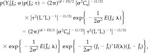(28)

where

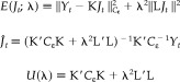
and Because only the second exponential in equation (28) contains the integrand J _t, the integral can be evaluated in closed form as

We then obtain (−2) times Type II log‐likelihood as follows:

(29)

We have replaced the parameter τ by λ = σ/τ and constant terms have been ignored. The second and third terms of equation (29) can be simplified further by the singular value decomposition of K̄≡C _ε ^−1/2 KL⁻¹=USV′. The second term can be arranged as

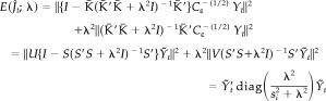(30)

where Ȳ _t=U′C _ε ^−1/2 Y _t, and s _i is the ith singular value in the matrix S. The third term can be simplified as

(31)

Substituting equations (30) and (31) into (29), we can finally obtain (−2) times Type II log‐likelihood as

where _i,t is ith component of the vector Ȳ _t. The hyperparameters λ, σ can be obtained in such way that the function −2l _t ^(II) will be minimized. Differentiating −2l _t ^(II) with respect to σ², the estimate of σ² is provided by

The regularization parameter λ can be obtained by minimizing

Because in the case of LORETA, the probability densities p(Y _t,J _t; σ,τ),t=1, …, T are serially independent, the (−2) Type II log‐likelihood based on T data points can be obtained as follows:

REFERENCES

- Akaike H (1980a): Likelihood and the Bayesian procedure In: Bernardo JM, Degroot MH, Lindley DV, Smith AFM, editors. Bayesian statistics. Valencia, Spain: University Press; p 141–166. [Google Scholar]
- Akaike H (1980b): Seasonal adjustment by a Bayesian modeling. J Time Series Anal 1: 1–13. [Google Scholar]
- Aoki M (1987): State space modeling of time series. Berlin: Springer. [Google Scholar]
- Backus G, Gilbert F (1968): The resolving power of gross earth data. Geophys J R Astron Soc 16: 169–205. [Google Scholar]
- Brooks DH, Ghandi F, Macleod RS, Maratos M (1999): Inverse electrocardiography by simultaneous imposition of multiple constraints. IEEE Trans Biomed Eng 46: 3–17. [DOI] [PubMed] [Google Scholar]
- Durbin J, Koopman SJ (2001): Time series analysis by state space models. Oxford: Oxford University Press. [Google Scholar]
- Galka A, Ozaki T, Yamashita O, Biscay R, Valdes‐Sosa P (2004): A solution to the dynamical inverse problem of EEG generation using spatiotemporal Kalman filtering. Neuroimage (in press). [DOI] [PubMed] [Google Scholar]
- Grave de Peralta Menendez R, Gonzalez Andino SL (1999): Backus and Gilbert method for vector fields. Hum Brain Mapp 7: 161–165. [DOI] [PMC free article] [PubMed] [Google Scholar]
- Grave de Peralta Menendez R, Gonzalez Andino SL (2002): Comparison of algorithms for localization of focal source evaluation with simulated data and analysis of experimental data. Int J Bioelectromagnetism 4 Online at http://www.rgi.tut.fi/jbem. [Google Scholar]
- Grave de Peralta Menendez R, Hauk O, Gonzalez Andino SL, Vogt H, Michel C (1997): Linear inverse solutions with optimal resolution kernels applied to electromagnetic tomography. Hum Brain Mapp 5: 454–467. [DOI] [PubMed] [Google Scholar]
- Hämäläinen MS, Ilmoniemi RJ (1984): Interpreting measured magnetic fields of the brain: estimates of current distributions. Technical Report TKK‐F‐A559. Helsinki: Helsinki University of Technology. [Google Scholar]
- Hansen PC (1992): Analysis of discrete ill‐posed problems by means of the L‐curve. SIAM Rev 34: 561–580. [Google Scholar]
- Hansen PC (1994): Regularization tools: a Matlab package for analysis and solution of discrete ill‐posed problems. Numerical Algorithms 6: 1–35. [Google Scholar]
- Jazwinski AH (1970): Stochastic processes and filtering theory. San Diego: Academic Press. [Google Scholar]
- Kaipio JP, Karjalainen PA, Somersalo E, Vauhkonen M (1999): State estimation in time‐varying electrical impedance tomography. Ann N Y Acad Sci 873: 430–439. [Google Scholar]
- Karjalainen PA, Vauhkonen M, Kaipio JP (1997): Dynamic reconstruction in SPET. In: Magnificent milestones and emerging opportunities in medical engineering. Proceedings of the 19th Annual International Conference of the IEEE Engineering in Medicine and Biology Society. Chicago, Oct. 30–Nov 2, 1997. p. 777–780.
- Kitagawa G, Gersh W (1996): Smoothness priors analysis of time series. New York: Springer. [Google Scholar]
- Mardia KV, Kent JT, Bibby JM (1979): Multivariate analysis. San Diego: Academic Press. [Google Scholar]
- Matsuura K, Okabe Y (1995): Selective minimum‐norm solution of the biomagnetic inverse problem. IEEE Trans Biomed Eng 42: 608–615. [DOI] [PubMed] [Google Scholar]
- Mazziotta JC, Toga A, Evans AC, Fox P, Lancaster J (1995): A probabilistic atlas of the human brain: theory and rationale for its development. Neuroimage 2: 89–101. [DOI] [PubMed] [Google Scholar]
- Nunez P (1981): Electric fields of the brain. New York: Oxford University Press. [Google Scholar]
- Pascual‐Marqui RD (1999): Review of methods for solving the EEG inverse problem. Int J Bioelectromagnetism 1: 75–86. [Google Scholar]
- Pascual‐Marqui RD, Michel CM (1994): LORETA: New authentic 3D functional images of the brain In: Skandies W, editor. ISBET Newsletter Giessen (GER) 5: 4–8. [Google Scholar]
- Pascual‐Marqui RD, Michel CM, Lehmann D (1994): Low resolution electromagnetic tomography: a new method for localizing electrical activity in the brain. Int J Psychophysiol 18: 49–65. [DOI] [PubMed] [Google Scholar]
- Phillips C, Rug MD, Friston KJ (2002): Systematic regularization of linear inverse solutions of the EEG source localization problem. Neuroimage 17: 287–301. [DOI] [PubMed] [Google Scholar]
- Riera JJ, Fuentes ME (1998): Electric lead field for a piecewise homogeneous volume conductor model of the head. IEEE Trans Biomed Eng 45: 746–753. [DOI] [PubMed] [Google Scholar]
- Rodin EA, Rodin MJ (1995): Dipole sources of the human alpha rhythm. Brain Topogr 7: 201–208. [DOI] [PubMed] [Google Scholar]
- Schmitt U, Louis AK (2002a): Efficient algorithms for the regularization of dynamic inverse problems: I. Theory. Inverse Problems 18: 645–658. [Google Scholar]
- Schmitt U, Louis AK (2002b): Efficient algorithms for the regularization of dynamic inverse problems: II. Applications. Inverse Problems 18: 659–676. [Google Scholar]
- Schmitt U, Louis AK, Darvas F, Buchner H, Fuchs M (2001): Numerical aspects of spatio‐temporal current density reconstruction from EEG‐/MEG‐data. IEEE Trans Med Imaging 20: 314–324. [DOI] [PubMed] [Google Scholar]
- Shumway RH (2000): Time series analysis and its applications. New York: Springer. [Google Scholar]
- Smith GD (1985): Numerical solution of partial differential equations: finite difference methods, Third ed. New York: Oxford University Press. [Google Scholar]
- Valdés‐Sosa P, Bosch J, Grave de Peralta‐Menendez R, Hernández JL, Pascual R, Biscay R (1992): Frequency domain models for the EEG. Brain Topogr 4: 309–319. [DOI] [PubMed] [Google Scholar]
- Vauhkonen PJ, Vauhkonen M, Kaipio JP (2001): Fixed‐lag smoothing in electrical impedance tomography. Int J Numerical Methods Eng 50: 2195–2209. [Google Scholar]
- Wahba G (1990): Spline models for observational data. Pennsylvania: Society for Industrial and Applied Mathematics. [Google Scholar]