Visual recognition of faces, objects, and words using degraded stimuli: Where and when it occurs

Abstract

We studied time course and cerebral localisation of word, object, and face recognition using event‐related potentials (ERPs) and source localisation techniques. To compare activation rates of these three categories, we used degraded images that easily pop out without any change in the physical features of the stimuli, once the meaning is revealed. Comparisons before and after identification show additional periods of activation beginning at 100 msec for faces and at around 200 msec for objects and words. For faces, this activation occurs predominantly in right temporal areas, whereas for objects, the specific time period gives rise to bilateral posterior but right dominant foci. Finally, words show a maximum area of activation in the left temporooccipital area at their specific time period. These results provide unequivocal evidence that when effects of low‐level visual features are circumvented, faces, objects, and words are not only distinct in terms of their anatomic routes, but also in terms of their times of processing. Hum. Brain Mapping 22:300–310, 2004. © 2004 Wiley‐Liss, Inc.

INTRODUCTION

Neuroscience has provided a good deal of evidence demonstrating that higher order brain regions involved in visual recognition differ depending on whether the class of stimuli presented are faces, objects, or words [for reviews, see Farah, 1994; Grüsser and Landis, 1991]. Differences in the timing of recognition between these categories are as yet unclear. Although several event‐related potential (ERP) and magnetoencephalographic (MEG) studies have been carried out to resolve this debate, a general consensus is lacking concerning possible timing differences in the processing of these categories [Bentin et al., 1996; Braeutigam et al., 2001; Cohen et al., 2000; Doniger et al., 2000; Eimer, 2000; Eimer and McCarthy, 1999; George et al., 1996; Jeffreys, 1989; Khateb et al., 2002; Liu et al., 2000; Sams et al., 1997; Schendan et al., 1998; Seeck et al., 1997; Streit et al., 2000; Tallon‐Baudry et al., 1997]. One important biasing effect stems from disparities in physical characteristics of the stimuli. Indeed, whether comparing between categories, or comparing category‐identification to neutral control conditions, a confounding effect appears. This derives from the fact that the categories themselves, as well as the control conditions, differ unavoidably in terms of their physical features, consequently making it impossible to compare them directly without the risk of being misled by effects of lower level visual analysis [VanRullen and Thorpe, 2001].

One way of tackling this problem has been by using degraded black and white images [Dolan et al., 1997; Landis et al., 1984; Tallon‐Baudry et al., 1997]. These stimuli are particularly interesting because both object recognition and control conditions are investigated using strictly identical visual scenes. In initial presentations, the stimuli are presented as black and white patches and blobs that seem meaningless to the observer. After this control condition, the objects hidden within the scene are revealed to the viewers and the same stimuli are then used again, this time as specific visual stimuli, such as faces or objects. Once the hidden meanings are revealed, they can no longer be ignored and subsequent presentations of the stimuli then lead to immediate identification [Tovee et al., 1996]. The meaning contained within the visual scene can only be extracted by activation of higher‐order cerebral processes that allow perceptual reorganisation of figure‐ground relationships and hence stimulus identification [Landis et al., 1984]. Any change in cerebral activity thus seems to be only assignable to object recognition per se and not to lower‐order visual processing.

In this study, using ERP map series analyses and source localisation methods, we investigated visual recognition of degraded images belonging to three stimulus categories (faces, objects and words), generally thought to be subserved by distinct neuronal networks [Farah, 1994; Grüsser and Landis, 1991].

It has been observed that the series of maps constituting an ERP do not fluctuate randomly but go through periods of relative stability (referred to as functional microstates) that likely reflect different steps of information processing in the brain [Khateb et al., 1999; Lehmann, 1987; Michel et al., 2001; Pegna et al., 1997]. This analysis relies on the assumption that any change in the configuration of the electric potential distribution on the scalp is due to a modification of the configuration of active sources in the brain [Lehmann, 1987]. Source localisation techniques can then be used to establish the cerebral areas responsible for these microstates. These methodologic procedures have been used successfully in several investigations [e.g., Ducommun et al., 2002; Khateb et al., 1999, 2001, 2002, 2003; Morand et al., 2000; Pegna et al., 1997, 2002; Schnider et al., 2002; Thut et al., 1999].

In our study, ERP map series were consequently analysed in terms of segments of quasi‐stable map topographies to identify microstates specific to each category of stimuli. We therefore compared successive segments of map topographies induced by degraded stimuli before and after their identification to determine when faces, objects, and words were processed. We then applied a distributed linear inverse solution [Grave de Peralta Menendez et al., 2001] to the relevant ERP maps to determine the location of the cerebral generators at critical times.

SUBJECTS AND METHODS

Subjects

Twenty medical students (ten men, age 25 ± 4 years) took part in the experiment, for which they were paid. All were right‐handed on the Oldfield‐Edinburgh scale (mean = 80.5 ± 18). They had normal or corrected‐to‐normal vision, were medication free and reported no history of psychiatric or neurologic disease (including problems in visual recognition or reading). Written, informed consent was provided before experimentation as recommended by the ethics committee of Geneva University Hospital.

Stimuli

The stimuli consisted of degraded images of two faces, two objects, and two words. The face images were those of one unknown male and one unknown female. The object images were two scanned photographs of musical instruments (a saxophone and a guitar). The words were two French nouns, chat and chien (cat and dog, respectively) written irregularly in large diagonal letters (150‐point Helvetica bold font). Except for the male face, which was taken from a previous experiment [Landis et al., 1984], the remaining stimuli were all created for this investigation. All stimuli were placed on a white rectangular 15 × 20 cm canvas using Adobe Photoshop (v. 5.5 for Macintosh). They were degraded first by adding a nonsense visual background, then by applying a 3–5‐pixel radius median filter replacement and subsequently transforming the images to black and white bitmaps. The final stimuli were therefore 20 × 15 cm unidentifiable bitmap images of faces, objects, and words. Examples of the three stimulus categories are shown in Figure 1A and their non‐degraded counterparts in Figure 1B. Finally, for the initial part of the experiment two distractors were created by distorting meaningless black/white bitmap images into spiralling shapes similar to the procedure used by Tallon‐Baudry et al. [1997].

Figure 1.

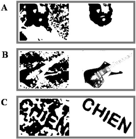
Examples of the three categories of stimuli used during ERP recordings. Left: Visual stimuli as presented during the ERP measures. Right: Where in the visual scene the actual stimuli are hidden. A, B, C: Examples of faces, objects, and words, respectively.

Procedure

The experiment was carried out in two consecutive electroencephalogram (EEG) recording runs. In the first run, each (as yet unrecognised) image and distractor was presented 25 times, yielding in total 200 pseudorandom stimuli composed of 50 presentations of unidentified faces (UF), 50 of unidentified objects (UO), 50 of unidentified words (UW), and 50 distractors. Subjects were asked to respond to “spiral” or “non‐spiral” by pressing one of two keys with the index and middle finger of their right hand. Half of the subjects responded to a spiral using the index finger whereas the other half used the middle finger.

At the end of this first run, hidden stimuli were revealed to the subjects by showing them the non‐degraded versions of each stimulus. The subjects were asked if they had identified them, or any other meaning, during the run. If such was the case, the subjects were excluded from further analysis. For the remaining subjects, paper printouts of the degraded images and their non‐degraded equivalents were provided and participants were asked to study them carefully until they felt certain they could easily recognise each stimulus. They were told that the remainder of the experiment required rapid identification of the degraded images.

After this familiarisation period, which usually lasted 10–15 min, a second EEG run was carried out during which the subjects responded to faces (referred to as IF), objects (IO), or words (IW) using one of three keys with their right index, middle, and ring fingers (the registry between response finger and stimulus type again was counterbalanced across subjects). As during the first run, each stimulus category appeared 50 times.

In both EEG runs, stimuli were presented at the centre of the screen (120 cm distance; maximum 4.8‐degree eccentricity for the farthest borders of the images) using a Macintosh PowerPC 7200 running software for psychological testing (MacProbe; Aristometrics Computer Systems, Woodland Hills, CA). Stimuli were presented for 225 msec and were preceded for 675 msec by a central fixation point. A 675‐msec time window followed, during which the fixation cross was again visible and the subjects gave their response. Subjects were instructed to maintain their gaze on the fixation point at all times and to avoid any eye movements when the stimulus appeared.

EEG Recording Averaging

Continuous EEG was acquired at 500 Hz with a Geodesics system (Electrical Geodesics, Inc., Eugene, OR) from 125 scalp electrodes referenced to the vertex. Three electrooculograph (EOG) leads were used to monitor eye movements. Impedances were kept below 50 kΩ. The EEG was filtered offline from 1–30 Hz and recalculated against the average reference [Lehmann and Skrandies, 1980]. ERP epochs (from 40 msec pre‐ to 500 msec poststimulus onset) were averaged separately for each subject in UF, UO, and UW conditions (the first run), and in IF, IO, and IW conditions (the second run). The 40‐msec prestimulus epoch served to establish baseline. After excluding trials containing blinks, eye movements, or other artefacts (EEG sweeps with amplitude exceeding ±100 μV criterion) as well as trials with erroneous or absent behavioural responses from the analysis, the mean (± SD) of artefact‐free trials obtained in UF, UO, UW, IF, IO, and IW was 38 ± 9 of 50, 39 ± 8 of 50, 43 ± 6 of 50, 43 ± 6 of 50, 42 ± 7 of 50 and 43 ± 7 of 50, respectively (F[5,70] = 1.86; P = 0.1).

ERP Map Series Analysis

Because our objective was to search for differences in brain responses to different categories of stimuli, a spatiotemporal analysis using a temporal segmentation procedure based on k‐means cluster analysis [Pascual‐Marqui et al., 1995] was first applied to the grand mean ERP map series (GM‐ERP). As described above, the segmentation procedure searches for periods of stable map configurations called microstates [Lehmann, 1987] or segment maps (SMs) within the in the GM‐ERP map series. This procedure allows the identification of SMs that are shared by the different conditions and those that are condition specific [Khateb et al., 2001, 2002; Michel et al., 2001; Pegna et al., 1997, 2002]. The algorithm is reference independent and is independent of amplitude modulations, because normalised data are compared.

Briefly, the algorithm proceeds in the following manner. A set of maps is selected randomly from the GM‐ERP as candidate SMs. At each time point in the GM‐ERP, the procedure substitutes the existing map with its closest matching SM. The times of onset and offset, as well as the total amount of variance explained by the SMs are then computed. The procedure is then reiterated with a new set of randomly selected SMs, and this process is repeated until the SMs that best explain the GM‐ERP data set are established.

This same segmentation procedure is then repeated over again, this time incrementing the number of SMs selected at onset. Once the procedure has been carried out for different numbers of SMs, a cross‐validation criterion is used to determine the number of SMs that should be retained at the final count [Pascual‐Marqui et al., 1995]. This criterion allows a non‐subjective determination of the smallest number of SMs explaining the greatest amount of variance.

This first step of analysis establishes differences in the grand mean ERPs. To determine the statistical relevance of these findings over individuals, however, a second analysis is needed. In this second step, each SM's presence is sought for every subject's ERPs using strength‐independent spatial correlation [Khateb et al., 1999, 2001, 2002; Pegna et al., 1997, 2002]. This is carried out by comparing the subject's scalp topography at each time point with the set of SMs obtained from the GM‐ERPs in step one. The map in the individual's ERP at each time point is then relabelled with the SM with which it correlates most highly. This procedure makes it possible to determine for every subject the onset of each SM, its total duration, and the amount of variance (as a percentage) they each explain over the whole time period [see Khateb et al., 1999; Pegna et al., 1997]. Statistical comparison of these parameters can then be carried out to establish whether different SMs better explain particular conditions.

Source Localisation Analysis

The last phase of analysis consists of determining the location of the electrical generators responsible for the SMs of interest. The active brain regions for each SM were estimated using a distributed linear inverse solution, based on a local auto‐regressive average (LAURA) model of the unknown current density in the brain [Grave de Peralta Menendez and Gonzalez Andino, 1999; Grave de Peralta Menendez et al., 2001]. LAURA uses a realistic head model with 4,024 lead field nodes equally distributed within the grey matter of the average brain of Statistical Parametric Mapping software (Wellcome Department, UK). Like other inverse solutions of this family, LAURA is capable of dealing with multiple simultaneously active sources of a priori unknown location [Michel et al., 2001; Pegna et al., 2002].

RESULTS

Five subjects (four subjects who spontaneously identified one of two hidden faces during the initial run and one who had numerous eye‐blinks and other artefacts on the EEG) were excluded from both behavioural and ERP analysis. Accordingly, the following analyses were carried out on the remaining 15 subjects (7 men and 8 women).

Behaviour

In the initial run, subjects categorised the distractors and stimuli with no difficulty (46 ± 3 of 50 hits for spirals, 48 ± 3 for UF, 48 ± 3 for UO, and 48 ± 3 for UW). Reaction times were slightly longer for distractors (465 ± 60) than for unidentified stimuli (448 ± 62 for UF, 450 ± 63 for UO, and 435 ± 54 for UW respectively). No significant difference, however, was found between the three unidentified conditions (F[2,28] = 2.11, P = 0.14) suggesting that all were perceived as meaningless stimuli. In the second session, after identification, the subjects continued to categorise the stimuli accurately (44 ± 7, 44 ± 9, and 42 ± 8 of 50 for faces, instruments, and words, respectively; F[2,28] = 0.34, P = 0.71). Response times were not statistically different across categories with 600 msec (± 67) for faces, 599 msec (± 68) for instruments, and 596 msec (± 55) for words (F[2,28] = 0.09, P = 0.92).

Electrophysiology

Preliminary analysis

To ensure that all unidentified stimuli (non‐spiralling) were actually perceived as meaningless black and white blobs and thus processed in the same nonspecific manner, we first carried out a preliminary analysis on the grand means of UF, UO, and UW conditions. For this purpose, the GM‐ERP maps series of these three unidentified conditions were subjected together to the temporal segmentation procedure. The rationale for this analysis was to test whether any stimulus‐specific processing had occurred (even unconsciously) during the first run and to determine its electrophysiologic correlates. As expected, the segmentation of UF, UO, and UW ERP map series revealed that the same five topographic template maps best explained all three GM‐ERPs. These maps were similarly found in five successive segments in UF, UO, and UW conditions (data not shown). On average, these segments occurred in the three conditions between 0–95 msec (first segment), 90 to ∼144 msec (second segment), 144 to ∼190 msec (third segment), 190 to ∼300 msec (fourth segment), and 300 to ∼500 msec (fifth segment). Based on this observation, indicating the absence of qualitative differences between the unidentified conditions in terms of map topography, the three conditions were collapsed into one single unidentified condition (UC) for further comparison with the identified conditions.

Topographical analysis by ERP map series segmentation

In this step of analysis, the four grand mean ERP map series (UC, IF, IO, and IW) were submitted to the temporal segmentation procedure described above to characterise segments that were shared by different conditions and those that appeared specifically in one or the other condition. The four grand mean map series were therefore entered into the modified cluster analysis to establish the SMs that explained all map series and those that were found only in specific conditions. A separate segmentation was carried out on the early part and the late part of the ERP, i.e., 0–200 msec and 200–500 msec. This yielded eight SMs that best explained the four ERP map series between 0–500 msec. Figure 2A displays each of the SMs. The four ERPs, with the 125 channels superimposed, are shown in Figure 2B with onsets and offsets of SMs indicated by arrows below as determined by the temporal segmentation. The only differences found between experimental conditions over the 500‐msec epoch in the GM‐ERPs were one additional SM specific to each category. SM2 appears for IF only, SM5 is found only for IO, and finally SM6 appears only in IW.

Figure 2.

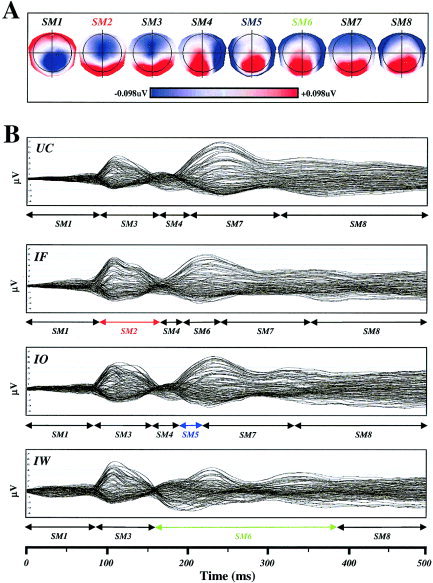
Results of ERP map series segmentation. A: Segment maps (SMs) for the eight scalp potentials, explaining the four grand mean ERP map series, are illustrated with positive values in red and negative values in blue. SM2 (red) was specific to faces and was named SMF. SM5 (blue) was specific to objects and was named SMO. Finally, SM6 (green) was specific to words and named SMW. B: Grand mean ERP traces (all 125 channels superimposed) are shown for the unidentified condition (UC), identified faces (IF), identified objects (IO), and identified words (IW) from top to bottom, respectively. Arrows below ERPs indicate the periods during which each SM was present.

Segment analysis in individual subjects

To establish statistical validity of these three specific SMs in ERPs of each individual, SM2–7 were submitted to further analysis. Because all four grand means began with SM1 (before the visual response) and terminated with SM8 (which occurred during motor response preparation; see RTs), these two SMs were not taken into consideration.

Every subject's ERP map series in the four conditions was therefore relabelled with the six SMs to determine: (1) the total time spent by each individual in each of these segments; (2) the global variance explained by each of the SMs in each condition; and (3) the time of map onsets (i.e., the first time point a given SM was found in each individual's ERPs). As seen in Table I (top), when fitting the maps to the subjects' data, all six SMs can be found at various durations in the individual ERP map series, even though in the GM‐ERP map series some maps appeared in one but not another condition. Statistical comparison of the durations of SM2–7 in all subjects using a 6 × 4 (SMs × experimental conditions) analysis of variance (ANOVA) showed a highly significant interaction between SM and condition (F[15,210] = 2.59; P < 0.001). This interaction indicated that the total time spent by each subject in each SM differed according categories. Post‐hoc, LSD tests on SMs of interest (namely SM2, SM5, and SM6) demonstrated that SM2 was present significantly more in IF as compared to that in IO, IW, or UC (P < 0.026; P < 0.003, and P < 0.014, respectively). SM5 was more present in IO than in IF and IW (P < 0.038 and P < 0.004). Finally, SM6 was more present in IW than in IF, IO, or UC (P < 0.008; P < 0.01, and P < 0.0002, respectively).

Table I.

Segment duration in milliseconds and segment global explained variance

	UC	IF	IO	IW
Segment duration
SM2a	53 (40)	98 (67)	57 (49)	44 (60)
SM3	77 (62)	54 (58)	67 (56)	57 (40)
SM4	15 (19)	38 (43)	20 (25)	34 (35)
SM5a	91 (84)	70 (73)	107 (87)	56 (58)
SM6a	49 (73)	70 (73)	71 (90)	118 (102)
SM7	18 (48)	24 (32)	23 (40)	16 (22)
Segment global explained variance
SM2a	0.08 (0.11)	0.19 (0.20)	0.08 (0.10)	0.08 (0.14)
SM3	0.18 (0.19)	0.09 (0.12)	0.15 (0.18)	0.14 (0.12)
SM4	0.01 (0.01)	0.01 (0.03)	0.01 (0.01)	0.01 (0.03)
SM5a	0.23 (0.25)	0.15 (0.15)	0.24 (0.24)	0.11 (0.16)
SM6a	0.03 (0.05)	0.04 (0.05)	0.04 (0.06)	0.07 (0.09)
SM7	0.05 (0.16)	0.05 (0.08)	0.04 (0.07)	0.03 (0.05)

Six of eight segment maps (SM2 to SM7) found in the grand mean event‐related potential (ERP) were sought in subjects' ERP map series for the four conditions (unidentified, UC; identified faces, IF; identified objects, IO; identified words, IW). The average time spent in each of these SMs is given in milliseconds with standard deviation in parentheses. The mean global explained variance (± standard deviation) by each one of SMs confirms the specificity of SM2 to faces, SM5 to objects, and SM6 to words.

^aThree segments (SM2, SM5, and SM6, indicated by an asterisk) were found to significantly differentiate the conditions in terms of their duration (significantly longer times indicated in bold).

We then compared global explained variance (reflecting the goodness‐of‐fit, i.e., how well the data were explained by a given map) of each segment map in each condition (Table I, bottom). As explained above, the selected SMs corresponded to the smallest number of maps explaining the greatest amount of variance in the GM‐ERPs. Due to the lower signal‐to‐noise ratio in the ERP map series of the individuals, a large amount of residual variance was expected when these SMs were used to explain them. Nevertheless, if a SM was specific to a given condition in the grand means, it should have also explained statistically more of the variance in the individuals' ERP in that same condition, despite the additional noise. We thus established the amount of variance explained by SM2–7 in the four ERP map series of every individual (i.e., how well each SM explained the ERPs of each individual) and compared these values using a 6 × 4 (SMs × experimental conditions) ANOVA. As expected, we observed a highly significant interaction between SM and condition (F[15,210] = 3.38; P < 0.0001) because some SMs explained certain conditions better than others. A post‐hoc LSD test confirmed that: SM2 explained more variance in the IF condition than in IO, IW, or UC conditions (P < 0.0004; P < 0.0005 and P < 0.0005, respectively); SM5 explained individual ERP map series in IO better than in IF and IW (P < 0.04 and P < 0.004); and SM6 explained IW data better than IF, IO, or UC data (P < 0.02, P < 0.02, and P < 0.01, respectively). Taken together, these results showed a specificity of SM2 for IF, SM5 for IO, and SM6 for IW, in terms of both segment duration (reflecting how often an SM was found in the individual data) and global explained variance (how well the individual data were explained by a given SM). Given this specificity, SM2, 5, and 6 were labelled SMF, SMO, and SMW, respectively.

Because the SMF, SMO, and SMW were dissimilar in terms of their timing, the differences in onset times were submitted to one‐way ANOVA with repeated measures across subjects. Onset times were statistically significant (F[2,28] = 7.41; P = 0.0026) with SMF appearing earlier (mean and standard error over subjects: 97 ± 12 msec) than did SMO (179 ± 37 msec) and SMW (204 ±33 msec; LSD post‐hoc, P = 0.003 and P = 0.002, respectively). SMO and SMW, however, did not differ (LSD post‐hoc, P = 0.872).

Source Localisation

The generators responsible for SMF, SMO, and SMW were determined using the source localisation algorithm LAURA (Fig. 3). When subjected to LAURA, the SMF yielded a right temporal gyrus activation, with a small secondary source in the left parietal region as shown in Figure 3A. SMO showed bilateral regions of activation (Fig. 3B), with a clear maximum in the right lingual and middle occipital gyri and symmetrical secondary sources on the left. Finally, SMW yielded a maximum in the posterior left lingual and middle occipital gyri, with a small secondary right source in the posterior cingulum (Fig. 3C).

Figure 3.

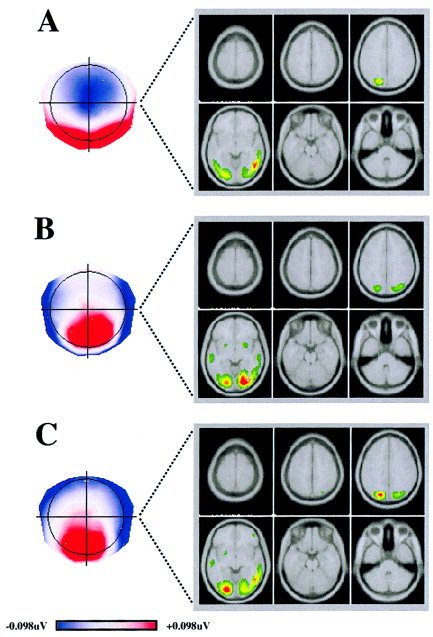
Source localisation. A, B, C: Estimations obtained using the distributed linear source localisation (LAURA) procedure for the segment maps specific to faces (SMF), objects (SMO), and words (SMW), respectively. The current density (green, low current density; red, high current density) maxima are shown on six horizontal slices of the average brain. SMF shows right temporal gyrus activation, with a small secondary source in left parietal region. SMO shows bilateral regions of activation, maximal in right lingual and middle occipital gyri and with a symmetrical secondary source on the left. For SMW, a maximum is found in posterior left lingual and middle occipital gyri, with a small secondary right source in posterior cingulum.

DISCUSSION

As expected, conscious perception of a stimulus within an initially apparently meaningless visual scene leads to additional higher‐tier brain activity, an observation made previously using other techniques [Bar et al., 2001; Dolan et al., 1997; Grill‐Spector et al., 2000; Landis et al., 1984; Tallon‐Baudry et al., 1997]. In this report, however, the additional activity was found category specific, with respect to both timing and cerebral localisation.

When the newly revealed object was a face, the significant electrical map topography began close to 100 msec with its generators predominating in right posterior areas. For objects and words, significant activity occurred later, beginning at around 180–200 msec for both categories, and was dominant in posterior right cerebral regions for the former and posterior left for the latter.

Our findings for faces were at odds with intracranial electrophysiologic investigations that have reported a face‐specific N200 from electrodes situated mainly at ventral occipitotemporal sites [Allison et al., 1994, 1999; Puce et al., 1999], and ERP studies describing the earliest response to faces at around 170 msec, the so‐called N170, characterised by a vertex‐positive and bilateral temporal‐negative deflection [Bentin et al., 1996; Eimer, 2000; Eimer and McCarthy, 1999; George et al., 1996; Jeffreys, 1989; Liu et al., 2000; Sams et al., 1997]. This component has in fact been described for a broad spectrum of face‐related stimuli, including schematically drawn faces [Sagiv and Bentin, 2001] or pairs of small shapes, primed to be seen as eyes [Bentin et al., 2002].

This time period for face processing has been challenged by several reports suggesting earlier processing times for faces [Braeutigam et al., 2001; Schendan et al., 1998; Seeck et al., 1997; Streit et al., 2000]. Unfortunately, in these reports, differences due to the more basic visual properties of the stimuli cannot altogether be ruled out [VanRullen and Thorpe, 2001]. In our investigation, the stimuli were identical before and after recognition, thus excluding an interpretation in terms of low‐level differences and speaking in favour of a specific period for face recognition, with onset as early as 100 msec.

The possibility that intracranial investigations may have overlooked an earlier response cannot be ruled out, partly because data are limited by spatial sampling of electrode penetrations. For example, Puce et al. [1999] failed to find any difference between familiar and unfamiliar faces in the first 700 msec of their recordings, yet behavioural studies show that recognition does take place by that time [Faulkner et al., 2002]. The intracranial recordings reported above could thus reflect a later response to face processing. In agreement with this suggestion is the fact that their electrophysiologic responses were bilateral, whereas the early responses found in our investigation [as well as in studies such as Braeutigam et al., 2001; Seeck et al., 1997] were lateralised to the right. Our investigation thus would support further the hypothesis of an initial right‐lateralised response followed by a bilateral activation for faces [Seeck et al., 2001].

Nonetheless, surface electric and magnetic recordings have also reported slightly later responses for faces. Based on a MEG study, Tarkiainen et al. [2002] argued recently that two distinct processes occur in the first 200 msec of face and letter processing, based on the presence of two separable patterns of activation. These investigators presented letter‐strings in a first experiment, then schematic faces in a follow‐up study, in which various levels of visual noise were added. They observed an initial pattern of activation that reacted to the visual complexity of the stimulus (which they determined based on the amount of noise and the number of items composing the stimulus). This activation, which they call Type I, appeared in the first 100 msec with sources estimated in the midline occipital area. The second pattern of activation (called Type II) appeared at 150 msec and was related to the type of stimulus (i.e., face, word). Sources for Type II activation were found in inferior occipitotemporal cortex, left lateralised for words and bilateral with a slight right dominance for faces. This suggests that the initial lower‐level visual processing (Type I) is identical for both types of stimuli, whereas the stimulus‐specific processing (Type II), takes place in anatomically distinct regions at similar times (after 150 msec) for both categories. At first glance, our results do not seem to agree with the investigation by Tarkiainen et al. [2002]. Two possible reasons could explain the apparent discrepancy. In contrast to methods relying on component analyses, our observations are based on extraction of stable map topographies that are defined by onsets and offsets, which may obviously include these components. Our results thus may not necessarily contradict investigations that find components peaking shortly after our SM onsets, but might simply reflect differences in points of focus, as is partially the case here. Nevertheless, the investigators may also have overlooked an earlier response for faces. Tarkiainen et al. [2002] considered the greater signal strength associated with increasing levels of noise as a sign of Type I (i.e., lower‐level) processing. Under these noisy viewing conditions, however, the visual system must perceptually fill in progressively greater amounts of missing information for stimulus identification to occur. Along these lines, it has been shown that the perception of incomplete (illusory) figures produces stronger signals in higher‐tier cortical areas related to object recognition [Larsson et al., 1999; Mendola et al., 1999; Pegna et al., 2002]. An increase in signal strength associated with greater visual noise, such as that observed by Tarkiainen et al. [2002], may not necessarily mean that the activity is purely low‐level, precluding any possible higher‐order stimulus‐specific activity. Because the authors defined Type I activity in faces as an early (<130 msec) source showing a systematic increase in amplitude with the amount of noise, and then defined Type II as sources peaking after Type I but before 200 msec, it remains a possibility that at least part of the early response could have been specific to faces.

Indeed, in another recent MEG study, a result similar to ours has been reported by Liu et al. [2002]. These investigators found a response over temporooccipital sensors around 100 msec after face presentation that could not be attributed to low‐level features of the stimulus. By adding visual noise to the stimuli, Liu et al. [2002] were able to determine that the magnetic response was correlated with the subject's capacity to categorise the stimulus as a face, but not with the subject's capacity to recognise the individuals that were depicted. By contrast, the response at 170 msec was correlated with both these processes. The initial response thus seems related to recognition, whereas the latter involves identification of an individual face. These results provide a possible interpretation for the absent or very weak N170 in our results. As our face stimuli were degraded to avoid immediate recognition, we would surmise that the process of degradation might have rendered any identification impossible, thus excluding this later process along with its electrophysiologic signature.

The right hemisphere dominance yielded by our source localisation procedure during the processing of face stimuli concurs with several studies involving for example functional magnetic resonance imaging (fMRI) and MEG or patients with cerebral damage [e.g., De Renzi, 2000; De Renzi et al., 1994; Farah, 1994; Gauthier et al., 1999; Kanwisher et al., 1997; Swithenby et al., 1998]. An additional right middle temporal activation for faces has been observed also in the intracranial investigations mentioned above [Puce et al., 1996] although at a later period in time. Interestingly, in a paradigm very similar ours, Dolan et al. [1997] used degraded images of faces and objects while measuring fMRI activation and evidenced a right superior temporal response when comparing faces to objects, an activation that they attributed to category‐specific recognition processes.

In ERP studies, the time course related to identification of objects turns out to be highly similar to ours when drawings of objects with different levels of fragmentation are used. For example, we have shown recently [Khateb et al., 2002] that scrambled line drawings differed from whole images by the appearance of an additional map topography beginning at around 280 msec. Along similar lines, Doniger et al. [2000] presented line drawings at different degrees of fragmentation and compared the ERPs obtained before and after recognition. Significant changes began at approximately 230 msec, mainly over lateral occipitotemporal sites. They suggested that the regions activated at this point were situated in the lateral occipital areas of both hemispheres. These regions have been associated with object recognition, whether the stimuli are complete [Malach et al., 1995] or defined by illusory contours [Mendola et al., 1999; Murray et al., 2002; Pegna et al., 2002]. The bilateral, right‐dominant activation obtained in this study is thus concordant with although somewhat more posterior than are the bilateral occipital regions reportedly involved in object recognition.

Tallon‐Baudry et al. [1997] reported somewhat different results using an EEG paradigm. The investigators presented a similarly degraded image of a Dalmatian hidden in a noisy black and white visual scene to their subjects who were asked to respond to spiral‐shaped targets. Once the hidden dog was revealed, the procedure was carried out again and subjects were asked to count either the occurrences of the dog or the spiralling forms amidst distractors. A differential effect was found, in the form of a posterior negativity peaking around 290 msec. The response was observed after target presentation, whether these were constituted by a dog or a spiralling shape. Consequently, Tallon‐Baudry et al. [1997] attributed this effect to the spatial filtering of irrelevant information in the presence of a target. Because our effects were seen earlier and the scalp topography was different, our results must reflect prior processes relating to object recognition, whereas their responses could reflect events pertaining to production and inhibition of responses taking place after stimulus identification [Jackson et al., 1999; Jodo and Kayama, 1992; Pfefferbaum et al., 1985].

Likewise, the posterior left hemisphere implication of word recognition that we obtain is coherent with data from brain‐damaged patients who present pure alexia after left posterior brain injury [Damasio and Damasio, 1983; see also Farah, 1994 or Grüsser and Landis, 1991 for reviews]. Imagery studies have also implicated the left occipitotemporal cortex as a region responsible for processing visual linguistic information [Buchel et al., 1998; Petersen et al., 1990; Price et al., 1996; Price and Friston, 1997; Puce et al., 1996]. This left basal temporal region has been termed the visual word‐form area (VWF) and seems to be involved primarily in processing letter strings [Cohen et al., 2000]. Using ERP analyses, Cohen et al. suggested that the activation of this area during visuo‐verbal processing appeared at around 180–200 msec. Comparisons between words and non‐words showed a difference beginning at 200 msec. Our previous data comparing ERP responses to images and words also demonstrated that the earliest differences in map topographies between these two types of stimuli begin at around 200 msec [Khateb et al., 2002].

By opposition, intracranial ERP recordings [Allison et al., 1994; Nobre et al., 1994] found electrical responses to letter strings in the posterior fusiform gyri on both sides, which peaked at around 200 msec. The timing of this activity was somewhat earlier than that in our observations, because the peak coincided with onset of our SM6. Nobre et al. [1994] noted that their response, found over certain electrode sites only, was specific to letter strings, including non‐words, and was independent of the semantic content. Furthermore, these electrode sites did not yield the characteristic N200 response for other types of visual stimuli (including faces and objects). The authors posit that the neural processing in this area over the first 200 msec could reflect the formation of word percepts on a prelexical level.

When comparing surface ERPs to numerous stimuli, including words, non‐words, and pseudo‐font strings, Schendan et al. [1998] found differences as early as 150 msec, suggesting that visual categorisation on a prelexical, perceptive level may occur even sooner. The amplitude and scalp distribution at 150 msec, however, was similar for both faces and words. This contradicts the evidence showing that distinct neural networks process these two categories of stimuli. Their results may thus reflect processing on a lower perceptual level (such as stimulus familiarity, as suggested by the authors themselves), whereas ours occur at a category‐specific level. Along similar lines, Tarkiainen et al. [1999, 2002] observed activation around 150 msec after stimulus presentation over left occipitotemporal sensors in a MEG study using letter strings. The authors note that these responses were also present for non‐word letter strings or strings of rotated letters, suggesting that the response was possibly an indication of processing of element strings rather than word processing per se. This offers an interpretation for our slightly later responses, considering that our stimuli were composed of meaningful words.

The regions of activation observed in our investigation, associated with the stimuli we employed, may lead one to conjecture about a possible implication of lateral temporal motion sensitive areas. Indeed, the superior and middle temporal gyri have been shown to be sensitive not only to real motion but also to static images with implied motion [Kourtzi and Kanwisher, 2000], static faces [Chao et al., 1999; Kanwisher et al., 1997], and manipulable objects [Chao et al, 1999]. Taken together, these investigations demonstrated that responses to faces were situated in the superior temporal gyrus and responses to manipulable objects in the middle temporal gyri. Our patterns of activation are not consistent with these areas of activation and thus cannot simply reflect the response of motion areas to our static stimuli. Furthermore, although such static images may activate lateral temporal motion areas, the levels of activation are probably weaker than are those produced by areas involved in recognition per se [Beauchamp et al., 2002]. More importantly, motion sensitive areas would not be expected to show any clear category‐specific timing differences or hemispheric lateralisation such as those observed in our data.

The use of degraded images in our investigation has allowed us to study the temporal progression of brain function during the processing of each category of stimuli while circumventing potential effects linked to their low‐level physical characteristics. This procedure confirmed that face, object, and word processing depend on anatomically distinct neural systems. Our first and foremost demonstration, however, was that these systems processed their data at different times. Under identical conditions, faces were processed earlier than were objects or words, demonstrating further that faces form a privileged category of stimuli. This is quite plausible, because faces constitute a class of highly relevant stimuli, both biologically and socially. Such relevance may require the activation of different cortical pathways. Indeed, a growing body of evidence now suggests that facial expressions of emotions are processed through a colliculo‐pulvinar route to the amygdala [see for example, de Gelder et al., 1999; Morris et al., 1999, 2001]. This information concerning facial expressions may be conveyed in parallel to face recognition and more rapidly, as suggested by electrophysiologic methodologies [Eger et al., 2003; Eimer and Holmes, 2002; Pizzagalli et al., 1999]. One could therefore speculate that, at least where faces are concerned, the geniculate route may be supplemented by a secondary, extrageniculate pathway could yield a quicker, cruder analysis to evaluate possible biological relevance or threat. Such a process might include perception of relevance on a broader level, such as the mere presence of a face, without recognition.

REFERENCES

- Allison T, McCarthy G, Nobre A, Puce A, Belger A (1994): Human extrastriate visual cortex and the perception of faces, words, numbers, and colors. Cereb Cortex 4: 544–554. [DOI] [PubMed] [Google Scholar]
- Allison T, Puce A, Spencer DD, McCarthy G (1999): Electrophysiological studies of human face perception. I: Potentials generated in occipitotemporal cortex by face and non‐face stimuli. Cereb Cortex 9: 415–430. [DOI] [PubMed] [Google Scholar]
- Bar M, Tootell RB, Schacter DL, Greve DN, Fischl B, Mendola JD, Rosen BR, Dale AM (2001): Cortical mechanisms specific to explicit visual object recognition. Neuron 29: 529–535. [DOI] [PubMed] [Google Scholar]
- Beauchamp MS, Lee KE, Haxby JV, Martin A (2002): Parallel visual motion processing streams for manipulable objects and human movements. Neuron 34: 149–159. [DOI] [PubMed] [Google Scholar]
- Bentin S, Allison T, Puce A, Perez E, McCarthy G (1996): Electrophysiological studies of face perception in humans. J Cogn Neurosci 8: 551–565. [DOI] [PMC free article] [PubMed] [Google Scholar]
- Bentin S, Sagiv N, Mecklinger A, Friedrici A, von Cramon DY (2002): Priming visual face‐processing mechanisms: electrophysiological evidence. Psychol Sci 13: 190–193. [DOI] [PubMed] [Google Scholar]
- Braeutigam S, Bailey AJ, Swithenby SJ (2001): Task‐dependent early latency (30–60 ms) visual processing of human faces and other objects. Neuroreport 12: 1531–1536. [DOI] [PubMed] [Google Scholar]
- Buchel C, Price C, Friston K (1998): A multimodal language region in the ventral visual pathway. Nature 394: 274–277. [DOI] [PubMed] [Google Scholar]
- Chao LL, Haxby JV, Martin A (1999): Attribute‐based neural substrates in temporal cortex for perceiving and knowing about objects. Nat Neurosci 2: 913–919. [DOI] [PubMed] [Google Scholar]
- Cohen L, Dehaene S, Naccache L, Lehericy S, Dehaene‐Lambertz G, Henaff MA, Michel F (2000): The visual word form area: spatial and temporal characterization of an initial stage of reading in normal subjects and posterior split‐brain patients. Brain 123: 291–307. [DOI] [PubMed] [Google Scholar]
- Damasio AR, Damasio H (1983): The anatomic basis of pure alexia. Neurology 33: 1573–1583. [DOI] [PubMed] [Google Scholar]
- de Gelder B, Vroomen J, Pourtois G, Weiskrantz L (1999): Non‐conscious recognition of affect in the absence of striate cortex. Neuroreport 10: 3759–3763. [DOI] [PubMed] [Google Scholar]
- De Renzi E (2000): Disorders of visual recognition. Semin Neurol 20: 479–485. [DOI] [PubMed] [Google Scholar]
- De Renzi E, Perani D, Carlesimo GA, Silveri MC, Fazio F (1994): Prosopagnosia can be associated with damage confined to the right hemisphere—an MRI and PET study and a review of the literature. Neuropsychologia 32: 893–902. [DOI] [PubMed] [Google Scholar]
- Dolan RJ, Fink GR, Rolls E, Booth M, Holmes A, Frackowiak RS, Friston KJ (1997): How the brain learns to see objects and faces in an impoverished context. Nature 389: 596–599. [DOI] [PubMed] [Google Scholar]
- Doniger GM, Foxe JJ, Murray MM, Higgins BA, Snodgrass JG, Schroeder CE, Javitt DC (2000): Activation timecourse of ventral visual stream object‐recognition areas: high density electrical mapping of perceptual closure processes. J Cogn Neurosci 12: 615–621. [DOI] [PubMed] [Google Scholar]
- Ducommun CY, Murray MM, Thut G, Bellmann A, Viaud‐Delmon I, Clarke S, Michel CM (2002): Segregated processing of auditory motion and auditory location: an ERP mapping study. Neuroimage 16: 76–88. [DOI] [PubMed] [Google Scholar]
- Eger E, Jedynak A, Iwaki T, Skrandies W (2003): Rapid extraction of emotional expression: evidence from evoked potential fields during brief presentation of face stimuli. Neuropsychologia 41: 808–817. [DOI] [PubMed] [Google Scholar]
- Eimer M (2000): The face‐specific N170 component reflects late stages in the structural encoding of faces. Neuroreport 11: 2319–2324. [DOI] [PubMed] [Google Scholar]
- Eimer M, McCarthy RA (1999): Prosopagnosia and structural encoding of faces: evidence from event‐related potentials. Neuroreport 10: 255–259. [DOI] [PubMed] [Google Scholar]
- Farah MJ (1994): Visual agnosia: disorders of object recognition and what they tell us about normal vision. Cambridge: MIT Press. [Google Scholar]
- Faulkner TF, Rhodes G, Palermo R, Pellicano E, Ferguson D (2002): Recognizing the un‐real McCoy: priming and the modularity of face recognition. Psychon Bull Rev 9: 327–334. [DOI] [PubMed] [Google Scholar]
- Gauthier I, Tarr MJ, Anderson AW, Skudlarski P, Gore JC (1999): Activation of the middle fusiform “face area” increases with expertise in recognizing novel objects. Nat Neurosci 2: 568–573. [DOI] [PubMed] [Google Scholar]
- George N, Evans J, Fiori N, Davidoff J, Renault B (1996): Brain events related to normal and moderately scrambled faces. Brain Res Cogn Brain Res 4: 65–76. [DOI] [PubMed] [Google Scholar]
- Grave de Peralta Menendez R, Gonzalez Andino S (1999): Distributed source models. Standard solutions to new developments In: Uhl C, editor. Analysis of neurophysiological brain functioning. Heidelberg: Springer; p 176–201. [Google Scholar]
- Grave de Peralta Menendez R, Gonzalez Andino S, Lantz G, Michel CM, Landis T (2001): Noninvasive localization of electromagnetic epileptic activity. I. Method descriptions and simulations. Brain Topogr 14: 131–137. [DOI] [PubMed] [Google Scholar]
- Grill‐Spector K, Kushnir T, Hendler T, Malach R (2000): The dynamics of object‐selective activation correlate with recognition performance in humans. Nat Neurosci 3: 837–843. [DOI] [PubMed] [Google Scholar]
- Grüsser OJ, Landis T (1991): Visual agnosias and other disturbances of visual perception and cognition. London: MacMillan Press; 610 p. [Google Scholar]
- Jackson SR, Jackson GM, Roberts M (1999): The selection and suppression of action: ERP correlates of executive control in humans. Neuroreport 10: 861–865. [DOI] [PubMed] [Google Scholar]
- Jeffreys DA (1989): A face‐responsive potential recorded from the human scalp. Exp Brain Res 78: 193–202. [DOI] [PubMed] [Google Scholar]
- Jodo E, Kayama Y (1992): Relation of a negative ERP component to response inhibition in a Go/No‐go task. Electroencephalogr Clin Neurophysiol 82: 477–482. [DOI] [PubMed] [Google Scholar]
- Kanwisher N, McDermott J, Chun MM (1997): The fusiform face area: a module in human extrastriate cortex specialized for face perception. J Neurosci 17: 4302–4311. [DOI] [PMC free article] [PubMed] [Google Scholar]
- Khateb A, Annoni J, Landis T, Pegna AJ, Custodi MC, Fonteneau E, Morand SM, Michel CM (1999): Spatio‐temporal analysis of electric brain activity during semantic and phonological word processing. Int J Psychophysiol 32: 215–231. [DOI] [PubMed] [Google Scholar]
- Khateb A, Michel CM, Pegna AJ, Thut G, Landis T, Annoni JM (2001): The time course of semantic category processing in the cerebral hemispheres: an electrophysiological study. Brain Res Cogn Brain Res 10: 251–264. [DOI] [PubMed] [Google Scholar]
- Khateb A, Michel CM, Pegna AJ, O'Dochartaigh SD, Landis T, Annoni JM (2003): Processing of semantic categorical and associative relations: an ERP mapping study. Int J Psychophysiol 49: 41–55. [DOI] [PubMed] [Google Scholar]
- Khateb A, Pegna AJ, Michel CM, Landis T, Annoni JM (2002): Dynamics of brain activation during an explicit word and image recognition task: an electrophysiological study. Brain Topogr 14: 197–213. [DOI] [PubMed] [Google Scholar]
- Kourtzi Z, Kanwisher N (2000): Activation in human MT/MST by static images with implied motion. J Cogn Neurosci 12: 48–55. [DOI] [PubMed] [Google Scholar]
- Landis T, Lehmann D, Mita T, Skrandies W (1984): Evoked potential correlates of figure and ground. Int J Psychophysiol 1: 345–348. [DOI] [PubMed] [Google Scholar]
- Larsson J, Amiunts K, Gulyas B, Malikovic A, Zilles K, Roland PE (1999): Neuronal correlates of real and illusory contour perception: functional anatomy with PET. Eur J Neurosci 11: 4024–4036. [DOI] [PubMed] [Google Scholar]
- Lehmann D, Skrandies W (1980): Reference‐free identification of components of checkerboard‐evoked multichannel potential fields. Electroencephalogr Clin Neurophysiol 48: 609–621. [DOI] [PubMed] [Google Scholar]
- Lehmann D (1987): Principles of spatial analysis In: Gevins AS, Remond A, editors. Handbook of electroencephalography and clinical neurophysiology. Vol 1 Methods of analysis of brain electrical and magnetic signals. Amsterdam: Elsevier; p 309–354. [Google Scholar]
- Liu J, Harris A, Kanwisher N (2002): Stages of processing in face perception: an MEG study. Nat Neurosci 5: 910–916. [DOI] [PubMed] [Google Scholar]
- Liu J, Higuchi M, Marantz A, Kanwisher N (2000): The selectivity of the occipitotemporal M170 for faces. Neuroreport 11: 337–341. [DOI] [PubMed] [Google Scholar]
- Malach R, Reppas JB, Benson RR, Kwong KK, Jiang H, Kennedy WA, Ledden PJ, Brady TJ, Rosen BR, Tootell RB (1995): Object‐related activity revealed by functional magnetic resonance imaging in human occipital cortex. Proc Natl Acad Sci USA 92: 8135–8139. [DOI] [PMC free article] [PubMed] [Google Scholar]
- Mendola JD, Dale AM, Fischl B, Liu AK, Tootell RB (1999): The representation of illusory and real contours in human cortical visual areas revealed by functional magnetic resonance imaging. J Neurosci 19: 8560–8572. [DOI] [PMC free article] [PubMed] [Google Scholar]
- Michel CM, Thut G, Morand S, Khateb A, Pegna AJ, Grave de Peralta R, Gonzalez S, Seeck M, Landis T (2001): Electric source imaging of human brain functions. Brain Res Brain Res Rev 36: 108–118. [DOI] [PubMed] [Google Scholar]
- Morand S, Thut G, de Peralta RG, Clarke S, Khateb A, Landis T, Michel CM (2000): Electrophysiological evidence for fast visual processing through the human koniocellular pathway when stimuli move. Cereb Cortex 10: 817–825. [DOI] [PubMed] [Google Scholar]
- Morris JS, DeGelder B, Weiskrantz L, Dolan RJ (2001): Differential extrageniculostriate and amygdala responses to presentation of emotional faces in a cortically blind field. Brain 124: 1241–1252. [DOI] [PubMed] [Google Scholar]
- Morris JS, Ohman A, Dolan RJ (1999): A subcortical pathway to the right amygdala mediating “unseen” fear. Proc Natl Acad Sci USA 96: 1680–1685. [DOI] [PMC free article] [PubMed] [Google Scholar]
- Murray MM, Wylie GR, Higgins BA, Javitt DC, Schroeder CE, Foxe JJ (2002): The spatiotemporal dynamics of illusory contour processing: combined high‐density electrical mapping, source analysis, and functional magnetic resonance imaging. J Neurosci 22: 5055–5073. [DOI] [PMC free article] [PubMed] [Google Scholar]
- Nobre AC, Allison T, McCarthy G (1994): Word recognition in the human inferior temporal lobe. Nature 372: 260–263. [DOI] [PubMed] [Google Scholar]
- Pascual‐Marqui RD, Michel CM, Lehmann D (1995): Segmentation of brain electrical activity into microstates: Model estimation and validation. IEEE Trans Biomed Eng 42: 658–665. [DOI] [PubMed] [Google Scholar]
- Pegna AJ, Khateb A, Spinelli L, Seeck M, Landis T, Michel CM (1997): Unraveling the cerebral dynamics of mental imagery. Hum Brain Mapp 5: 410–421. [DOI] [PubMed] [Google Scholar]
- Pegna AJ, Khateb A, Murray MM, Landis T, Michel CM (2002): Neural processing of illusory and real contours revealed by high‐density ERP mapping. Neuroreport 13: 965–968. [DOI] [PubMed] [Google Scholar]
- Pizzagalli D, Regard M, Lehmann D (1999): Rapid emotional face processing in the human right and left brain hemispheres: an ERP study. Neuroreport 10: 2691–2698. [DOI] [PubMed] [Google Scholar]
- Petersen SE, Fox PT, Snyder AZ, Raichle ME (1990): Activation of extrastriate and frontal cortical areas by visual words and word‐like stimuli. Science 249: 1041–1044. [DOI] [PubMed] [Google Scholar]
- Pfefferbaum A, Ford JM, Weller BJ, Kopell BS (1985): ERPs to response production and inhibition. Electroencephalogr Clin Neurophysiol 60: 423–434. [DOI] [PubMed] [Google Scholar]
- Price CJ, Friston KJ (1997): Cognitive conjunction: a new approach to brain activation experiments. Neuroimage 5: 261–270. [DOI] [PubMed] [Google Scholar]
- Price CJ, Wise RJ, Frackowiak RS (1996): Demonstrating the implicit processing of visually presented words and pseudowords. Cereb Cortex 6: 62–70. [DOI] [PubMed] [Google Scholar]
- Puce A, Allison T, Asgari M, Gore JC, McCarthy G (1996): Differential sensitivity of human visual cortex to faces, letterstrings, and textures: a functional magnetic resonance imaging study. J Neurosci 16: 5205–5215. [DOI] [PMC free article] [PubMed] [Google Scholar]
- Puce A, Allison T, McCarthy G (1999): Electrophysiological studies of human face perception. III: Effects of top‐down processing on face‐specific potentials. Cereb Cortex 9: 445–458. [DOI] [PubMed] [Google Scholar]
- Sagiv N, Bentin S (2001): Structural encoding of human and schematic faces: holistic and part‐based processes. J Cogn Neurosci 13: 1–15. [DOI] [PubMed] [Google Scholar]
- Sams M, Hietanen JK, Hari R, Ilmoniemi RJ, Lounasmaa OV (1997): Face‐specific responses from the human inferior occipito‐temporal cortex. Neuroscience 77: 49–55. [DOI] [PubMed] [Google Scholar]
- Schendan HE, Ganis G, Kutas M (1998): Neurophysiological evidence for visual perceptual categorization of words and faces within 150 ms. Psychophysiology 35: 240–251. [PubMed] [Google Scholar]
- Schnider A, Valenza N, Morand S, Michel CM (2002): Early cortical distinction between memories that pertain to ongoing reality and memories that don't. Cereb Cortex 12: 54–61. [DOI] [PubMed] [Google Scholar]
- Seeck M, Michel CM, Mainwaring N, Cosgrove R, Blume H, Ives J, Landis T, Schomer DL (1997): Evidence for rapid face recognition from human scalp and intracranial electrodes. Neuroreport 8: 2749–2754. [DOI] [PubMed] [Google Scholar]
- Seeck M, Michel CM, Blanke O, Thut G, Landis T, Schomer DL (2001): Intracranial neurophysiological correlates related to the processing of faces. Epilepsy Behav 2: 545–557. [DOI] [PubMed] [Google Scholar]
- Streit M, Wolwer W, Brinkmeyer J, Ihl R, Gaebel W (2000): Electrophysiological correlates of emotional and structural face processing in humans. Neurosci Lett 278: 13–16. [DOI] [PubMed] [Google Scholar]
- Swithenby SJ, Bailey AJ, Brautigam S, Josephs OE, Jousmaki V, Tesche CD (1998): Neural processing of human faces: a magnetoencephalographic study. Exp Brain Res 118: 501–510. [DOI] [PubMed] [Google Scholar]
- Tallon‐Baudry C, Bertrand O, Delpuech C, Permier J (1997): Oscillatory gamma‐band (30–70 Hz) activity induced by a visual search task in humans. J Neurosci 17: 722–734. [DOI] [PMC free article] [PubMed] [Google Scholar]
- Tarkiainen A, Cornelissen PL, Salmelin R (2002): Dynamics of visual feature analysis and object‐level processing in face versus letter‐string perception. Brain 125: 1225–1136. [DOI] [PubMed] [Google Scholar]
- Tarkiainen A, Helenius P, Hansen PC, Cornelissen PL, Salmelin R (1999): Dynamics of letter string perception in the human occipitotemporal cortex. Brain 122: 2119–2132. [DOI] [PubMed] [Google Scholar]
- Thut G, Hauert CA, Morand S, Seeck M, Landis T, Michel C (1999): Evidence for interhemispheric motor‐level transfer in a simple reaction time task: an EEG study. Exp Brain Res 128: 256–261. [DOI] [PubMed] [Google Scholar]
- Tovee MJ, Rolls ET, Ramachandran VS (1996): Rapid visual learning in neurones of the primate temporal visual cortex. Neuroreport 7: 2757–2760. [DOI] [PubMed] [Google Scholar]
- VanRullen R, Thorpe SJ (2001): The time course of visual processing: from early perception to decision‐making. J Cogn Neurosci 13: 454–461. [DOI] [PubMed] [Google Scholar]