

Abstract
We describe a method for the statistical parametric mapping of low resolution electromagnetic tomography (LORETA) using high‐density electroencephalography (EEG) and individual magnetic resonance images (MRI) to investigate the characteristics of the mismatch negativity (MMN) generators in schizophrenia. LORETA, using a realistic head model of the boundary element method derived from the individual anatomy, estimated the current density maps from the scalp topography of the 128‐channel EEG. From the current density maps that covered the whole cortical gray matter (up to 20,000 points), volumetric current density images were reconstructed. Intensity normalization of the smoothed current density images was used to reduce the confounding effect of subject specific global activity. After transforming each image into a standard stereotaxic space, we carried out statistical parametric mapping of the normalized current density images. We applied this method to the source localization of MMN in schizophrenia. The MMN generators, produced by a deviant tone of 1,200 Hz (5% of 1,600 trials) under the standard tone of 1,000 Hz, 80 dB binaural stimuli with 300 msec of inter‐stimulus interval, were measured in 14 right‐handed schizophrenic subjects and 14 age‐, gender‐, and handedness‐matched controls. We found that the schizophrenic group exhibited significant current density reductions of MMN in the left superior temporal gyrus and the left inferior parietal gyrus (P < 0. 0005). This study is the first voxel‐by‐voxel statistical mapping of current density using individual MRI and high‐density EEG. Hum. Brain Mapping 17:168–178, 2002. © 2002 Wiley‐Liss, Inc.
Keywords: mismatch negativity, statistical parametric mapping, LORETA, current density model
INTRODUCTION
The mismatch negativity (MMN) that appears after subtracting event related potential (ERP) of standard stimulus from that of deviant stimulus is reported to arise in 100–150 msec after stimulus onset and reach a maximum at around 200–250 msec. After reports that MMN does not rely on attention to the stimuli, MMN activities have been interpreted as representing a preattentive stage of auditory information processing [Näätänen et al., 1978], or an automatic neuronal‐mismatch process with a neuronal representation of the standard stimulus [Mantysalo and Näätänen, 1987.
MMN generators have been suspected to be located mainly in the primary auditory cortex or in its vicinity according to the results of MEG/EEG studies [Alho et al., 1998; Hari et al., 1984; Sams et al., 1985], functional magnetic resonance imaging (fMRI) [Opitz et al., 1999; Wible et al., 2001] and intracranial recording [Kropotov et al., 1995]. Since Näätänen and Michie [1979] first suggested the existence of two separate MMN generators, (i.e., the sensory‐specific generator and the frontal generator), there have been many reports of multiple MMN generators including at the frontal [Deouell et al., 1998; Giard et al., 1990] and parietal lobes [Kasai et al., 1999; Levanen et al., 1996].
Because MMN is related to the automatic passive discriminative process, and because schizophrenic patients show defects primarily in attentive functions, the occurrence of MMN in schizophrenics has been actively researched. Several studies have shown decreased amplitude [Catts et al., 1995; Hirayasu et al., 1998; Javitt et al., 1995; Shelley et al., 1991] and delayed latency [Shutara et al., 1996] of MMN activity in schizophrenic patients, although others have indicated no reduction [Kathmann et al., 1995; O'Donnell et al., 1994]. The attenuation of MMN in schizophrenics is thought to be associated with a deficit in pre‐attentive auditory processing [Javitt et al., 1993; 1991, 1999].
Although it is often assumed that MMN reflects a distributed network involving the auditory, prefrontal, and parietal cortex, relatively few studies have addressed the issue of which MMN source locations are affected in patients with schizophrenia. Furthermore, most of these studies were based on two‐dimensional scalp topography restricted to a small number of electrodes, which might provide low or somewhat distorted information on the source location.
To overcome the limitation of scalp topography, the last decade has seen the development of several current‐density estimation techniques whose goal is to find the location of the three‐dimensional (3D) intracerebral activities by solving an inverse problem; in other words, to ascertain the current density distribution inside the brain from the results of scalp EEG. Because of the infinite number of solutions that are possible due to the larger number of locations than that of sensors, 'constraint' needs to be used to find an optimal solution. Among several available constraint methods, LORETA (low‐resolution electromagnetic tomography) [Pascual‐Marqui et al., 1994] is one of the most widely used methods for the solution of inverse problems. The constraint used in LORETA is the determination of the spatially smoothest current distribution by applying a Laplacian operator to the current density. The LORETA assumption of greatest smoothness has acquired a growing mass of evidence as to its accuracy, including the results of intracranial study [Lantz et al., 1997].
As is typical in group comparison studies, statistical evaluation is essential. Such evaluation of current density is not yet relatively well established, as compared to positron emission tomography (PET) or fMRI studies, both of which have mainly employed the voxel‐based general linear model (GLM) using statistical parametric mapping (SPM). Nevertheless, the statistical comparison of current densities encounters similar problems to those of the PET or functional magnetic resonance imaging (fMRI) approaches. One is the compensation for anatomical variations between subjects, and another is the determination of the critical threshold for assigning significant difference in the multiple comparisons.
A common way to reduce anatomical variation is to co‐register each subject's electrodes to one standard brain image and to calculate current density on the standard image. LORETA‐KEY, developed in the Key Institute for Brain–Mind Research [Pascual‐Marqui et al., 1999], is the representative tool of this approach. Variable resolution electrical tomography (VARETA) [Bosch‐Bayard et al., 2001] also follows the same approach. Both LORETA‐KEY and VARETA use either the Talairach human brain atlas [Talairach and Tournoux, 1988] or the average map masked by the probability map, produced by the Montreal Neurological Institute [Evans et al., 1994], as a standard brain image. This standard brain image is used to constrain source locations to the cortical gray matter and the hippocampus, and a spherical head model with a low number of electrodes (19 for LORETA, 28 for VARETA, in previous publications) is utilized. After spatial normalization resulting from mapping EEG into one standard image, several voxel‐based statistical comparison methods have been used. In LORETA‐KEY, voxel‐by‐voxel t‐test [Pascual‐Marqui et al., 1999], and paired‐sample t‐test with subsequent binomial test [Anderer et al., 2000] have been used. Randomization was also employed to overcome the model assumption of the parametric method [Mulert et al., 2001].
The template‐based statistical comparisons such as LORETA‐KEY and VARETA, however, retain some limitations. Simulation studies have shown that the boundary element method (BEM) using individual MRI is more accurate than the spherical head model in solving the dipole source model [Buchner et al., 1995; Cuffin, 1996; Leahy et al., 1998; Waberski et al., 1998]. Similar results can be expected in the current density model. Also, high density sensors featuring more than 128 channels may be required to produce a significant reduction in estimation errors, according to previous reports [Babiloni et al., 1996; Srinivasan et al., 1996].
We investigated the characteristics of the MMN generators in schizophrenics by developing a method for the voxel‐based statistical parametric mapping of current density images, using individual MRI and high‐density EEG. We applied LORETA using 128‐channel EEG recordings and individual MRI, based on the realistic head model of BEM.
SUBJECTS AND METHODS
Subjects
Fourteen right‐handed schizophrenic patients (9 male, 5 female) were recruited from the Schizophrenia Clinic at the Department of Psychiatry, Seoul National University Hospital, Seoul, Korea. All patients met the DSM‐IV criteria for schizophrenia based on both Structured Clinical Interview for DSM‐IV (SCID‐IV) and psychiatric chart review. None of the patients had a history of electroconvulsive therapy, neurological illness, major head trauma, alcohol or drug abuse, or presently suffered auditory dysfunction. All patients were medicated, with a mean daily dose equivalent to 409 mg of chlorpromazine. The patients' mean age was 26.5 years (range 17–34), and their mean duration of illness was 5.4 years (range 1–16 years). Psychiatric symptoms were assessed with the Positive and Negative Syndrome Scale (PANSS). The mean of total scores from PANSS was 73 (range 54–96). The normal control group consisted of 14 age‐, gender‐, and handedness‐matched subjects who were recruited through internet advertisements. The controls also received SCID‐IV to rule out any major psychopathology. None of the controls had a history of neurological or psychiatric illness, or alcohol or drug abuse. The mean age of the control group was 24.6 years (range 19–42 years). There were no statistically significant differences between the two groups in parental socioeconomic status (normal controls, mean 3.3, standard deviation [SD] 0.7; patients, mean 3.3, SD 0.8) as measured by the Hollingshead two‐factor index of social position. All subjects gave written informed consent before participation in the study.
Source Localization of MMN
Stimulus procedure
The subjects were instructed to fix their eye on a single point on a blank video screen while sitting on a comfortable chair during the session. Tone pips of 80 dB SPL were presented binaurally to the subjects' ears via ear tips. Of the 1,600 total trials per session, 95% of trials were standard tones at 1,000 Hz, and 5% were deviant tones at 1,200 Hz. The plateau duration of the tone was 8 msec with rise and fall times of 1 msec and the interstimulus interval (ISI) was 300 msec. Subjects were asked to listen to the sounds without trying to distinguish or count.
EEG recordings
EEGs were recorded via a 128‐channel Quik‐cap (NeuroScan, El Paso, TX) with linked ears reference, using an ESI‐128 system (NeuroScan) in a dimly lit, soundproof, electrically shielded room at the Clinical Trial Center of Seoul National University Hospital. The electrode locations at the scalp were determined with a Isotrak 3D digitizer (Polhemus, Colchester, VT).
The sampling rate was 1,000 Hz/channel and the analog filter's band pass was 0.05–100 Hz. The epoch period of analysis was 300 msec, including a 50‐msec pre‐stimulus baseline. The baseline was corrected separately for each channel according to the mean amplitude of the EEG over the 50‐msec preceding stimulus onset. The EEG epochs that contained amplitudes exceeding ±75 μV at any EEG or EOG channels were automatically excluded from the averaging. The two average waveforms, obtained separately for the rare and frequent tonal stimuli, were digitally filtered with a band pass of 1–20 Hz using a Butterworth filter, order 5 in Curry v. 4.01 software (NeuroScan).
MMN was obtained by subtracting the ERPs of the standard stimuli from those of the deviant stimuli. The earlobe referenced MMN was transformed to common average reference. Artifact‐contaminated or bad electrodes (10% of total 128 channel on average) were removed by visual inspection for the application of LORETA.
Estimation of current densities using LORETA
Three‐dimensional T1‐weighted MR images were obtained for all subjects using 1.5‐T GE SIGNA Scanner (GE Medical Systems, Milwaukee, WI). A series of 124 contiguous sagittal images were acquired with the following parameters: TR = 11.2 msec, TE = 2.1 msec, 20‐degree flip angle, 24‐cm field of view, and matrix = 256 × 256. The voxel (volume of pixel) dimensions were 0. 9375 × 0. 9375 × 1.5 mm, which were resampled to be isocubic, i.e., 0. 9375 × 0. 9375 × 0. 9375 mm. LORETA was calculated with Curry v. 4.01 after matching the electrode locations with individual MRI. Three referential points, the nasion, left and right pre‐auricular points, were used for the matching the electrode locations with MRI.
We used a three‐compartment boundary element model (BEM) [Fuchs et al., 1998] by modeling the surface of the skin, the outside (skull), and the inside of the skull (liquor) with a total of 4,000 triangle nodes. The conductivities of the skin (10 mm), skull (9 mm), and liquor (7 mm) were 0.33, 0. 0042, and 0.33, respectively. Sources were constrained to be at least 3 mm inside the liquor/skull boundary and source locations were calculated in the cortex gray matter utilizing the rotating model. We calculated LORETA at a peak time point of the mean global field power (MGFP) of MMN at each subject. All peaks were located around 100–200 msec from the stimulus onset.
Statistical Evaluation
Spatial normalization and intensity normalization of current density
Current densities were calculated at the locations of whole cortical gray matter using LORETA. The number of individual locations was around 18,000–20,000 according to the volume size of each subject's cortex. The average distance between neighboring locations was about 1–2 mm. Note that the locations of current densities were not discrete grid voxels as produced by PET or MRI. Although each location had four parameter values (i.e., current orientation vector and its intensity), in this study only the intensity of the current density at each location was used for statistical comparison. To apply voxel‐based statistical comparison of the current density, the following steps were carried out.
Image reconstruction.
A current density image was reconstructed by filling a volume with the current intensities at the voxels corresponding to the locations of LORETA. The volume was same‐sized and same‐orientated with an individual MRI. This approach is similar to the method of VARETA [Bosch‐Bayard et al., 2001; Picton et al., 1999].
Gaussian smoothing.
The current density image was smoothed by convolving an isotropic Gaussian kernel with 12 mm FWHM (full width half maximum) to fill in‐between gray matter voxels that do not have corresponding locations of LORETA during volume construction. This spatial smoothing also increases the signal‐to‐noise ratio and accommodates the subtle variations in anatomical structures [Worsley et al., 1996a].
Spatial normalization.
Spatial normalization of the current density image was carried out using SPM99 (Institute of Neurology, University College of London, UK) implemented in Matlab (Mathworks, Newton, MA) [Ashburner and Friston, 1999]. All reconstructed current density images were transformed into a standard stereotactic anatomical space to remove the inter‐subject anatomical variability [Friston et al., 1995b]. Normalization parameters, firstly derived from the affine transformation and nonlinear warping of each subject's MRI to the MNI template, were then applied to the current density image. Affine transformation was carried out to determine the 12 optimal parameters for registration of the brain MRI on the standard template. Subtle differences between the transformed image and the template were eliminated by a nonlinear registration method using the weighted sum of the pre‐defined smooth basis functions used in discrete cosine transformation. The resultant image dimension was 79 × 95 × 68 and the unit size of one voxel was 2 × 2 × 2 mm.
Intensity normalization.
The main purpose of the source localization in the cognitive task is to estimate the regional activity (i.e., intensity) irrelevantly to the global activity of the cortical lobes. In practice, however, regional activity can be confounded by global activity that varies over a wide extent throughout subjects or groups. This variability may be due to the subject‐ or group‐specific neural characteristics. To reduce the confounding effects of subject specific activity, proportional scaling [Fox et al., 1988; Friston et al., 1990] has been a widely used method for PET studies. The basic assumption is that local electrical or metabolic activities are proportional to global activity for each subject. The proportional scaling method can be represented by a simple equation, y = x/a, where local activation (y) is equal to global activation (x) divided by a constant multiplication of the global activation (a). But in the analysis of EEG current densities, we thought that the extension of proportional scaling should be required to model the characteristics of current density derived from the inverse solution, which tends to have a focused, sparse distribution (super‐Gaussian). The extended proportional scaling can be represented as y = x/a + b, where the global mean of current densities (a) was calculated over the cortical gray matter and the baseline offset (b) was calculated by averaging the lower quartile of all current intensities.
Statistical parametric mapping
In comparing MMN generators of schizophrenic patients and controls, statistical parametric mapping with two‐sample t‐test was applied to the normalized current density images using SPM99. SPM99 is based on the estimation of the general linear model and on the interpretation of the model parameters at each voxel [Friston et al., 1995a]. Because of multiple comparison problems, SPM99 uses Gaussian random field theory [Friston et al., 1996; Worsley et al., 1996b] to protect against family‐wise false positivities over the search volume. The random field correction, or adjustment to the P‐values derived from continuous spatially extended data, plays the same role as the Bonferroni correction for discrete (e.g., single voxel) data. Critically, it accommodates spatial non‐sphericity or correlations among the error terms in a way that the Bonferroni correction would not.
For reference purposes, MMN generators of each group were investigated separately using one‐sample t‐test with the alternate hypothesis that the mean current density would be significantly different from global mean for a regionally specific generator. Because we set global mean as one, all voxel values subtracted by one were used for one‐sample t‐test.
We also analyzed a region of sphere with radius 32 mm, covering the superior temporal gyrus, using the small volume correction (SVC) in SPM99 [Worsley et al., 1996b]. This SVC analysis is a hypothesis‐driven approach based on the strong hypothesis that the superior temporal, prefrontal, and parietal regions are involved in MMN generation as reviewed in the introduction.
The whole procedures for statistical comparison of current density images are summarized in Figure 1.
Figure 1.
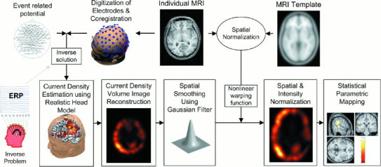
Procedural diagram of voxel‐based statistical evaluation of MMN current density. Current densities derived from LORETA at a peak time point of MMN constituted a volume image. As a step of intensity normalization, proportional scaling was applied to the current density images that were spatially normalized to a template. Average of 152 T1‐image produced by the Montreal Neurological Institute was used as a MRI template. Voxel‐based statistical parametric mapping was carried out using SPM99.
RESULTS
Figure 2 shows the statistical parametric map of t‐statistic (SPM{t}) of MMN generators in each group. This figure registers statistic map thresholded at T > 3.85 (P < 0.001) with contiguous 100‐voxel extent. MMN sources for the control subjects extended from the superior parietal lobule [Brodmann area (BA) 7] to the superior temporal gyrus (STG, BA 22) and the inferior frontal gyrus (BA 46) in the left hemisphere. The peak of grand‐average current density was found at the left inferior parietal lobule (IPL, BA 40) in the controls.
Figure 2.
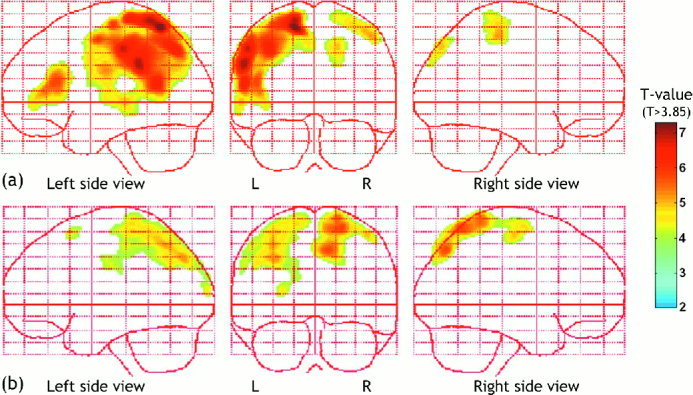
Statistical parametric map of t statistic (SPM{t}) of MMN in control subjects (a) and schizophrenia (b). Statistical map of one‐sample T‐test displays MMN activations of each group, normal control group in (a) and schizophrenia group in (b). Under the null hypothesis that there are no regional specific generators, the current density will be distributed around global mean by virtue of the global normalization. Under the alternate hypothesis of a regionally specific generator the mean current density will be significantly different from global mean. These images were thresholded at T > 3.85 (P < 0.001). In control, MMN sources extend from the superior parietal area (BA 7) to superior temporal gyrus (BA22) and inferior frontal gyrus (BA 46) in the left hemisphere. MMN sources of schizophrenia were located at superior parietal area (BA 7) bilaterally with reduced activity (b).
The results of the two sample t‐tests between the control and schizophrenia groups are presented in Table I, along with the anatomical location of those clusters with significantly reduced areas of current density in schizophrenia patients, the x, y, and z Talairach coordinates of the voxel with the maximum excursion, the highest Z‐value, and the voxel number (k) of the cluster. The threshold of significance for the clusters was defined as that containing at least 50 contiguous voxels exceeding a T value of 3.71, which corresponds to an uncorrected significance level of 0. 0005. The estimated smoothness was (23.4, 27.1, 27.2) mm and the search volume is 53.1 resolution elements with one resolution element being 2,150.27 voxels (2 × 2 × 2 mm). P values corrected by entire volume at both the voxel and cluster levels failed to meet a significance level of 0.05.
Table I.
Area with reduced current density of mismatch negativity in schizophrenia
| Region (BD) | Coordinates | Z (T) | k | P‐voxel | P‐cluster | ||
|---|---|---|---|---|---|---|---|
| Left STG (22) | −54 | −28 | 2 | 3.89 (4.58) | 93 | 0.016 (0.136) | 0.045 (0.304) |
| Left IPL (40) | −56 | −38 | 30 | 3.77 (4.40) | 340 | 0.024 (0.192) | 0.024 (0.103) |
STG, superior temporal gyrus; IPL, inferior parietal lobule; BD, Brodmann area. Coordinates refer to the 3 axes (x, y, z) of the Talairach coordinate system in mm. Z (T) and k refer to the maximum excursion in Z‐value (T‐value) and the cluster extent of uncorrected P < 0. 0005 with extent threshold = 50 voxels, respectively. P‐voxel and P‐cluster indicate the corrected P‐value at the voxel level and cluster level, respectively with small volume correction (SVC). P‐values with entire brain volume correction are in parentheses.
With small volume correction, the current density in STG of schizophrenic patients showed significant reduction as compared to the comparison subjects with P = 0.016 (corrected) for the voxel level and P = 0.045 (corrected) for the cluster level. The reduction of current density in IPL of schizophrenic patients showed significant (P = 0.024, corrected) at both the voxel level and cluster levels. In this case, the search volume had 17,157 voxels and, based on the smoothing kernel, eight resolution elements. Corrected P‐values at the voxel level and cluster level, respectively, are also displayed in Table I.
Figure 3 illustrates the statistically reduced current density area in the schizophrenia group compared to the control. As seen in Figure 3, the MMN density sources showing the greatest reduction are located in the left STG (Talairach coordinates −54/−28/2, BA 22). Reduction in the left inferior parietal lobule (BA 40) was also found in the schizophrenia group.
Figure 3.
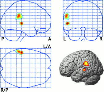
Statistical parametric maps displaying decreased current density of mismatch negativity in schizophrenia. Significantly deactivated areas (T > 3.71, P < 0. 0005 uncorrected, extent k > 50) of MMN sources in schizophrenia compared to control subjects are shown on the Talairach coordinate. MMN source reduction was found at the left superior temporal gyrus (Talairach coordinates −54/−28/2; BA 22) and the left inferior parietal lobule (−56/−38/30; BA 40). We could not find any significantly more activated area of MMN sources in schizophrenia with P < 0. 0005. Right bottom images displayed the reduced MMN activation regions in schizophrenia on the rendered image.
There was no evidence of any significantly increased MMN current density sources (P < 0. 0005) in the schizophrenia group compared to the controls.
DISCUSSION
Statistical analysis of 3D current density using individual MRI: methodological considerations
We used a framework of voxel‐based statistical comparison of current densities. Our method features two major advantages when compared to the previous current density comparison methods. First, we used the individual MRI‐based BEM model that was designed to reduce current distortion due to any anatomical differences. Previous statistical evaluations of current density [Bosch‐Bayard et al., 2001; Pascual‐Marqui et al., 1999] have largely been done on a standard image (MNI average template) without using individual MRI. Although no exact comparison has been previously drawn between using individual anatomy and using standard anatomy in establishing a conductivity model, it is not difficult to address the advantages of the individual MRI‐based BEM model due to its consideration of diverse anatomical differences between subjects and, thus, conductive distortion. Anatomical confounds caused by the usage of individual anatomy could be minimized by spatial normalization. Second, we used 128‐channel, high‐density EEG for estimation of current densities at cortical locations over 18,000 points. Several studies have implied that more than 128‐channel recording can provide higher spatial information and fewer localization errors [Babiloni et al., 1996; Srinivasan et al., 1996]. We believe that high density EEG is essentially required for the voxel‐based SPM that is affected largely by the accuracy of current density estimation.
SPM and the use of Gaussian corrections or adjustments to the P‐values are well suited for the analysis of LORETA current density estimates. This is because the smoothness induced by the constraints on the LORETA estimation causes profound spatial correlations among the data and errors that enter the statistical model. It is precisely these correlations that Gaussian field theory was designed to accommodate when adjusting the P‐values. Roughly speaking, this adjustment can be thought of as a Bonferroni correction for the number of resolution elements that is a function of the search volume and the smoothness of the data. Notice that this correction is neither a function of voxel size nor of the number of channels used in the original data acquisition.
The use of SPM implies that our data have normally distributed errors and conform to the assumptions used in parametric statistics. This is partly justified in our application because the errors are generated by inter‐subject variability, which we have no reason to assume are non‐Gaussian. Furthermore, the LORETA solution and smoothing that we applied to the data ensure that the errors are normally distributed through the central limit theorem. To check the assumption of normality, however, we replicated our analyses using the equivalent non‐parametric approach with SnPM (Statistical non‐Parametric Mapping) [Holmes et al., 1996]. As anticipated, the results were almost equivalent.
Further study is necessary concerning the use of voxel‐based SPM in the current density study. More elaboration is required on how to model the relationship between global activities and regional activities, and how to utilize the information of the current orientation. We believe that intensity normalization is one of most important issues in the statistical comparison of current densities like PET or fMRI data. No exact method has been suggested for intensity normalization of current density and no consensus exists. We used an extended proportional scaling method, but according to our experiment, SPM using the extended proportional scaling (y = x/a + b) showed no significant difference when compared to SPM using the general proportional scaling (y = x/a), indicating that the baseline offset (b) was almost zero in our MMN study. More theoretical and empirical elaboration should be undertaken.
MMN sources in the control
We found MMN generators were widely distributed in the left hemisphere of control subjects including IPL, STG, superior parietal lobule, and inferior frontal gyrus. According to the results presented in Figure 2a, the left inferior parietal lobule (IPL) was a major MMN source in control subjects. The involvement of right IPL in MMN generation has been reported by Levanen et al. [1996] and Kasai et al. [1999]. Levanen et al. [1996] thought that the right IPL might be related with modality‐independent change detection, and the superior temporal area with modality‐specific change detection. Contrary to this hypothesis, our study showed more pronounced MMN sources in the left IPL than in the right IPL. This finding of left hemispheric dominance in generating MMN is in accordance with that reported in the functional MRI study of Wible et al. [2001], which utilized the same stimulus as used in the present study. Despite the right–left discordance between Levanen's study and ours, IPL was involved in both studies.
In our study, the superior temporal gyrus (STG), which is the generally accepted location of the primary MMN generators, was also involved in MMN processing, although the SPM{t} was not as high as that of IPL. Relatively low activation in STG may be related with the selection of the MMN latency for calculation. Rinne et al. [2000] suggested that the MMN generator has the tendency to move anteriorly from STG to frontal lobe when the minimum norm estimation at the temporal peak and frontal peak was calculated. According to Rinne et al. [2000], MMN generators may be temporally moving sources and, therefore, MMN source location can be dependent on the definition of the latency time, used for calculating the current density. We calculated current densities at the peak time of the mean global field power of each subject's MMN by the average reference.
MMN sources in schizophrenia
In patients with schizophrenia, no consistent MMN sources were found at the left IPL and left STG, whereas most sources were located at the superior parietal lobule (BA 7). The reduced activity in the left hemisphere may represent a loss of hemispheric asymmetry. The presence of hemispheric asymmetry has been recognized by anatomical study in the auditory temporal region of healthy subjects [Galaburda et al., 1978a, b]. In schizophrenia, the loss of asymmetry has been reported by anatomical studies and ERP studies [Hajek et al., 1997; Kwon et al., 1999a; McCarley et al., 1993; Reite et al., 1989].
Our voxel‐based statistical comparison showed that schizophrenia was associated with a significant reduction of MMN current density in the left STG and the left IPL. Hirayasu et al. [1998], using the same modality as our study, reported abnormalities of the left parietotemporal junction in schizophrenia subjects, through surface topographical study. Javitt et al. [1993] also reported a deficit in the auditory cortical area of schizophrenia patients, with a tendency toward greater deficit in the left than right hemisphere. The reduced gray matter volume in the left STG of schizophrenia [O'Donnell et al., 1993; Shenton et al., 1993] may be related with the decreased MMN activity in the left STG of schizophrenia. Such findings of MMN amplitude reduction in the left STG support that schizophrenics have a deficit in the preattentive auditory sensory processing, which has been reported by several studies [Hirayasu et al., 1998; Kwon et al., 1999b; Shelley et al., 1991].
It should be noted that the activation maps in Figure 2 and Figure 3 were generated with the normalized images to focus on the regional activity of MMN sources relative to the global activity, specific to subject characteristics. The activated region can be interpreted with respect to both the current intensity and the spatial coincidence among subjects. Therefore, the highly activated region in SPM can be derived in one case where the highly activated region of each subject coincidentally overlaps throughout the group, whereas low activation may result from either of two possibilities, low activation or low coincidence, or possibly both. Therefore, we should not ignore the possibility that low activation in the left STG and left IPL of schizophrenia may be caused either by the various source distributions corresponding to the diverse spectrum of each subject in the schizophrenic group or by the widespread characteristics of sources in schizophrenia [Javitt et al., 1993].
We did not find any significant difference (P < 0. 0005, uncorrected, extent k = 50) of MMN frontal generators between schizophrenia patients and control groups even though relatively high statistical map was found at the left inferior frontal gyrus in controls.
CONCLUSION
This study is the first to try to develop a method for the statistical comparison of the current density model using individual MRI and high‐density EEG. By spatial normalization, we could reduce the anatomical effects caused by variations of individual anatomy, thus maintaining the conductivity head model of each subject. Intensity normalization was also carried out to reduce the subject specific global activity and to regulate the results within each group. After this, statistical comparison based on a general linear model and statistical inference was carried out. When applied to MMN, this framework showed substantial success in confirming a reduced current density in the left superior temporal gyrus and the left inferior parietal lobule in schizophrenia patients, a finding that agrees with those reported in previous studies.
REFERENCES
- Alho K, Winkler I, Escera C, Huotilainen M, Virtanen J, Jaaskelainen IP, Pekkonen E, Ilmoniemi RJ (1998): Processing of novel sounds and frequency changes in the human auditory cortex: magnetoencephalographic recordings. Psychophysiology 35: 211–224. [PubMed] [Google Scholar]
- Anderer P, Saletu B, Pascual‐Marqui RD (2000): Effect of the 5‐HT(1A) partial agonist buspirone on regional brain electrical activity in man: a functional neuroimaging study using low‐resolution electromagnetic tomography (LORETA). Psychiatry Res 100: 81–96. [DOI] [PubMed] [Google Scholar]
- Ashburner J, Friston KJ (1999): Nonlinear spatial normalization using basis functions. Hum Brain Mapp 7: 254–266. [DOI] [PMC free article] [PubMed] [Google Scholar]
- Babiloni F, Babiloni C, Carducci F, Fattorini L, Onorati P, Urbano A (1996): Spline Laplacian estimate of EEG potentials over a realistic magnetic resonance‐constructed scalp surface model. Electroencephalogr Clin Neurophysiol 98: 363–373. [DOI] [PubMed] [Google Scholar]
- Bosch‐Bayard J, Valdes‐Sosa P, Virues‐Alba T, Aubert‐Vazquez E, John ER, Harmony T, Riera‐Diaz J, Trujillo‐Barreto N (2001): 3D statistical parametric mapping of EEG source spectra by means of variable resolution electromagnetic tomography (VARETA). Clin Electroencephalogr 32: 47–61. [DOI] [PubMed] [Google Scholar]
- Buchner H, Waberski TD, Fuchs M, Wischmann HA, Wagner M, Drenckhahn R (1995): Comparison of realistically shaped boundary‐element and spherical head models in source localization of early somatosensory evoked potentials. Brain Topogr 8: 137–143. [DOI] [PubMed] [Google Scholar]
- Catts SV, Shelley AM, Ward PB, Liebert B, McConaghy N, Andrews S, Michie PT (1995): Brain potential evidence for an auditory sensory memory deficit in schizophrenia. Am J Psychiatry 152: 213–219. [DOI] [PubMed] [Google Scholar]
- Cuffin BN (1996): EEG localization accuracy improvements using realistically shaped head models. IEEE Trans Biomed Eng 43: 299–303. [DOI] [PubMed] [Google Scholar]
- Deouell LY, Bentin S, Giard MH (1998): Mismatch negativity in dichotic listening: evidence for interhemispheric differences and multiple generators. Psychophysiology 35: 355–365. [PubMed] [Google Scholar]
- Evans AC, Kamber M, Collins DL, Macdonald D (1994): An MRI‐based probabilistic atlas of neuroanatomy In: Shorvon S, Fish D, Andermann F, Bydder GM, Stefan H, editors. Magnetic resonance scanning and epilepsy. NATO ASI Series A, Life Sciences, Vol. 264 New York: Plenum. [Google Scholar]
- Fox PT, Mintun MA, Reiman EM, Raichle ME (1988): Enhanced detection of focal brain responses using intersubject averaging and change‐distribution analysis of subtracted PET images. J Cereb Blood Flow Metab 8: 642–653. [DOI] [PubMed] [Google Scholar]
- Friston KJ, Holmes A, Poline JB, Price CJ, Frith CD (1996): Detecting activations in PET and fMRI: levels of inference and power. Neuroimage 4: 223–235. [DOI] [PubMed] [Google Scholar]
- Friston KJ, Holmes AP, Worsley KJ, Poline JB, Frith CD, Frackowiak RS (1995a): Statistical parametric maps in functional imaging: a general linear approach. Hum Brain Mapp 2: 189–210. [Google Scholar]
- Friston KJ, Ashburner J, Frith CD, Poline JB, Heather JD, Frackowiak RS (1995b): Spatial registration and normalization of images. Hum Brain Mapp 2: 165–189. [Google Scholar]
- Friston KJ, Frith CD, Liddle PF, Dolan RJ, Lammertsma AA, Frackowiak RS (1990): The relationship between global and local changes in PET scans. J Cereb Blood Flow Metab 10: 458–466. [DOI] [PubMed] [Google Scholar]
- Fuchs M, Drenckhahn R, Wischmann HA, Wagner M (1998): An improved boundary element method for realistic volume‐conductor modeling. IEEE Trans Biomed Eng 45: 980–997. [DOI] [PubMed] [Google Scholar]
- Galaburda AM, LeMay M, Kemper TL, Geschwind N (1978a): Right–left asymmetrics in the brain. Science 199: 852–856. [DOI] [PubMed] [Google Scholar]
- Galaburda AM, Sanides F, Geschwind N (1978b): Human brain. Cytoarchitectonic left‐right asymmetries in the temporal speech region. Arch Neurol 35: 812–817. [DOI] [PubMed] [Google Scholar]
- Giard MH, Perrin F, Pernier J, Bouchet P (1990): Brain generators implicated in the processing of auditory stimulus deviance: a topographic event‐related potential study. Psychophysiology 27: 627–640. [DOI] [PubMed] [Google Scholar]
- Hajek M, Huonker R, Boehle C, Volz HP, Nowak H, Sauer H (1997): Abnormalities of auditory evoked magnetic fields and structural changes in the left hemisphere of male schizophrenics—a magnetoencephalographic‐magnetic resonance imaging study. Biol Psychiatry 42: 609–616. [DOI] [PubMed] [Google Scholar]
- Hari R, Hamalainen M, Ilmoniemi R, Kaukoranta E, Reinikainen K, Salminen J, Alho K, Näätänen R, Sams M (1984): Responses of the primary auditory cortex to pitch changes in a sequence of tone pips: neuromagnetic recordings in man. Neurosci Lett 50: 127–132. [DOI] [PubMed] [Google Scholar]
- Hirayasu Y, Potts GF, O'Donnell BF, Kwon JS, Arakaki H, Akdag SJ, Levitt JJ, Shenton ME, McCarley RW (1998): Auditory mismatch negativity in schizophrenia: topographic evaluation with a high‐density recording montage. Am J Psychiatry 155: 1281–1284. [DOI] [PubMed] [Google Scholar]
- Holmes AP, Blair RC, Watson JD, Ford I (1996): Nonparametric analysis of statistic images from functional mapping experiments. J Cereb Blood Flow Metab 16: 7–22. [DOI] [PubMed] [Google Scholar]
- Javitt DC, Doneshka P, Grochowski S, Ritter W (1995): Impaired mismatch negativity generation reflects widespread dysfunction of working memory in schizophrenia. Arch Gen Psychiatry 52: 550–558. [DOI] [PubMed] [Google Scholar]
- Javitt DC, Doneshka P, Zylberman I, Ritter W, Vaughan HG Jr (1993): Impairment of early cortical processing in schizophrenia: an event‐related potential confirmation study. Biol Psychiatry 33: 513–519. [DOI] [PubMed] [Google Scholar]
- Kasai K, Nakagome K, Itoh K, Koshida I, Hata A, Iwanami A, Fukuda M, Hiramatsu KI, Kato N (1999): Multiple generators in the auditory automatic discrimination process in humans. Neuroreport 10: 2267–2271. [DOI] [PubMed] [Google Scholar]
- Kathmann N, Wagner M, Rendtorff N, Engel RR (1995): Delayed peak latency of the mismatch negativity in schizophrenics and alcoholics. Biol Psychiatry 37: 754–757. [DOI] [PubMed] [Google Scholar]
- Kropotov JD, Naatnen R, Sevostianov AV, Alho K, Reinikainen K, Kropotova OV (1995): Mismatch negativity to auditory stimulus change recorded directly from the human temporal cortex. Psychophysiology 32: 418–422. [DOI] [PubMed] [Google Scholar]
- Kwon JS, McCarley RW, Hirayasu Y, Anderson JE, Fischer IA, Kikinis R, Jolesz FA, Shenton ME (1999a): Left planum temporale volume reduction in schizophrenia. Arch Gen Psychiatry 56: 142–148. [DOI] [PubMed] [Google Scholar]
- Kwon JS, O'Donnell BF, Wallenstein GV, Greene RW, Hirayasu Y, Nestor PG, Hasselmo ME, Potts GF, Shenton ME, McCarley RW (1999b): Gamma frequency‐range abnormalities to auditory stimulation in schizophrenia. Arch Gen Psychiatry 56: 1001–1005. [DOI] [PMC free article] [PubMed] [Google Scholar]
- Lantz G, Michel CM, Pascual‐Marqui RD, Spinelli L, Seeck M, Seri S, Landis T, Rosen I (1997): Extracranial localization of intracranial interictal epileptiform activity using LORETA (low resolution electromagnetic tomography). Electroencephalogr Clin Neurophysiol 102: 414–422. [DOI] [PubMed] [Google Scholar]
- Leahy RM, Mosher JC, Spencer ME, Huang MX, Lewine JD (1998): A study of dipole localization accuracy for MEG and EEG using a human skull phantom. Electroencephalogr Clin Neurophysiol 107: 159–173. [DOI] [PubMed] [Google Scholar]
- Levanen S, Ahonen A, Hari R, McEvoy L, Sams M (1996): Deviant auditory stimuli activate human left and right auditory cortex differently. Cereb Cortex 6: 288–296. [DOI] [PubMed] [Google Scholar]
- Mantysalo S, Näätänen R (1987): The duration of a neuronal trace of an auditory stimulus as indicated by event‐related potentials. Biol Psychol 24: 183–195. [DOI] [PubMed] [Google Scholar]
- McCarley RW, Shenton ME, O'Donnell BF, Faux SF, Kikinis R, Nestor PG, Jolesz FA (1993): Auditory P300 abnormalities and left posterior superior temporal gyrus volume reduction in schizophrenia. Arch Gen Psychiatry 50: 190–197. [DOI] [PubMed] [Google Scholar]
- Mulert C, Gallinat J, Pascual‐Marqui R, Dorn H, Frick K, Schlattmann P, Mientus S, Herrmann WM, Winterer G (2001): Reduced event‐related current density in the anterior cingulate cortex in schizophrenia. Neuroimage 13: 589–600. [DOI] [PubMed] [Google Scholar]
- Näätänen R, Gaillard AW, Mantysalo S (1978): Early selective‐attention effect on evoked potential reinterpreted. Acta Psychol (Amst) 42: 313–329. [DOI] [PubMed] [Google Scholar]
- Näätänen R, Michie PT (1979): Early selective‐attention effects on the evoked potential: a critical review and reinterpretation. Biol Psychol 8: 81–136. [DOI] [PubMed] [Google Scholar]
- O'Donnell BF, Hokama H, McCarley RW, Smith RS, Salisbury DF, Mondrow E, Nestor PG, Shenton ME (1994): Auditory ERPs to non‐target stimuli in schizophrenia: relationship to probability, task‐demands, and target ERPs. Int J Psychophysiol 17: 219–231. [DOI] [PubMed] [Google Scholar]
- O'Donnell BF, Shenton ME, McCarley RW, Faux SF, Smith RS, Salisbury DF, Nestor PG, Pollak SD, Kikinis R, Jolesz FA (1993): The auditory N2 component in schizophrenia: relationship to MRI temporal lobe gray matter and to other ERP abnormalities. Biol Psychiatry 34: 26–40. [DOI] [PubMed] [Google Scholar]
- Opitz B, Mecklinger A, Von Cramon DY, Kruggel F (1999): Combining electrophysiological and hemodynamic measures of the auditory oddball. Psychophysiology 36: 142–147. [DOI] [PubMed] [Google Scholar]
- Pascual‐Marqui RD, Lehmann D, Koenig T, Kochi K, Merlo MC, Hell D, Koukkou M (1999): Low resolution brain electromagnetic tomography (LORETA) functional imaging in acute, neuroleptic‐naive, first‐episode, productive schizophrenia. Psychiatry Res 90: 169–179. [DOI] [PubMed] [Google Scholar]
- Pascual‐Marqui RD, Michel CM, Lehmann D (1994): Low resolution electromagnetic tomography: a new method for localizing electrical activity in the brain. Int J Psychophysiol 18: 49–65. [DOI] [PubMed] [Google Scholar]
- Picton TW, Alain C, Woods DL, John MS, Scherg M, Valdes‐Sosa P, Bosch‐Bayard J, Trujillo NJ (1999): Intracerebral sources of human auditory‐evoked potentials. Audiol Neurootol 4: 64–79. [DOI] [PubMed] [Google Scholar]
- Reite M, Teale P, Goldstein L, Whalen J, Linnville S (1989): Late auditory magnetic sources may differ in the left hemisphere of schizophrenic patients. A preliminary report. Arch Gen Psychiatry 46: 565–572. [DOI] [PubMed] [Google Scholar]
- Rinne T, Alho K, Ilmoniemi RJ, Virtanen J, Näätänen R (2000): Separate time behaviors of the temporal and frontal mismatch negativity sources. Neuroimage 12: 14–19. [DOI] [PubMed] [Google Scholar]
- Sams M, Hamalainen M, Antervo A, Kaukoranta E, Reinikainen K, Hari R (1985): Cerebral neuromagnetic responses evoked by short auditory stimuli. Electroencephalogr Clin Neurophysiol 61: 254–266. [DOI] [PubMed] [Google Scholar]
- Shelley AM, Silipo G, Javitt DC (1999): Diminished responsiveness of ERPs in schizophrenic subjects to changes in auditory stimulation parameters: implications for theories of cortical dysfunction. Schizophr Res 37: 65–79. [DOI] [PubMed] [Google Scholar]
- Shelley AM, Ward PB, Catts SV, Michie PT, Andrews S, McConaghy N (1991): Mismatch negativity: an index of a preattentive processing deficit in schizophrenia. Biol Psychiatry 30: 1059–1062. [DOI] [PubMed] [Google Scholar]
- Shenton ME, O'Donnell BF, Nestor PG, Wible CG, Kikinis R, Faux SF, Pollak SD, Jolesz FA, McCarley RW (1993): Temporal lobe abnormalities in a patient with schizophrenia who has word‐finding difficulty: use of high‐resolution magnetic resonance imaging and auditory P300 event‐related potentials. Harv Rev Psychiatry 1: 110–117. [DOI] [PubMed] [Google Scholar]
- Shutara Y, Koga Y, Fujita K, Takeuchi H, Mochida M, Takemasa K (1996): An event‐related potential study on the impairment of automatic processing of auditory input in schizophrenia. Brain Topogr 8: 285–289. [DOI] [PubMed] [Google Scholar]
- Srinivasan R, Nunez PL, Tucker DM, Silberstein RB, Cadusch PJ (1996): Spatial sampling and filtering of EEG with spline Laplacians to estimate cortical potentials. Brain Topogr 8: 355–366. [DOI] [PubMed] [Google Scholar]
- Talairach J, Tournoux P (1988): Co‐planar stereotaxic atlas of the human brain. New York, NY: Thieme. [Google Scholar]
- Waberski TD, Buchner H, Lehnertz K, Hufnagel A, Fuchs M, Beckmann R, Rienacker A (1998): Properties of advanced head modelling and source reconstruction for the localization of epileptiform activity. Brain Topogr 10: 283–290. [DOI] [PubMed] [Google Scholar]
- Wible CG, Kubicki M, Yoo SS, Kacher DF, Salisbury DF, Anderson MC, Shenton ME, Hirayasu Y, Kikinis R, Jolesz FA, McCarley RW (2001): A functional magnetic resonance imaging study of auditory mismatch in schizophrenia. Am J Psychiatry 158: 938–943. [DOI] [PMC free article] [PubMed] [Google Scholar]
- Worsley KJ, Marrett S, Neelin P, Evans AC (1996a): Searching scale space for activation in PET images. Hum Brain Mapp 4: 74–90. [DOI] [PubMed] [Google Scholar]
- Worsley KJ, Marrett S, Neelin P, Vandal AC, Friston JJ (1996b): ). A unified statistical approach for determining significant voxels in images of cerebral activation. Hum Brain Mapp 4: 58–73. [DOI] [PubMed] [Google Scholar]