

Abstract
We investigated the decrease in intersubject functional variability in the horizontal meridian (HM) of the primary visual area (V1) before and after individual anatomical variability was significantly reduced using a high‐resolution spatial normalization (HRSN) method. The analyzed dataset consisted of 10 normal, right‐handed volunteers who had undergone both an O‐15 PET study, which localized retinotopic visual area (V1), and a high‐resolution anatomical MRI. Individual occipital lobes were manually segmented from anatomical images and transformed into a common space using an in‐house high‐resolution regional spatial normalization method called OSN. Individual anatomical and functional variability was quantified before and after HRSN processing. The reduction of individual anatomical variability was judged by the reduction in gray matter (GM) mismatch and by the improvement in overlap frequency between individual calcarine sulci. The reduction in intersubject functional variability of HM was determined by measurements of the overlap frequency between individual HM areas and by improvement in intersubject Z‐score maps. The HRSN processing significantly reduced the individual anatomical variability: GM mismatch was reduced by a factor of two and the mean calcarine sulcus overlap frequency was improved from 37 to 68%. The reduction in functional variability was more subtle. However, both HM mean overlap (increased from 18 to 28%) and the average Z‐score (increased from 2.2 to 2.55) were significantly improved. Although, functional registration was significantly improved by matching sulci, there was still residual variability. This is believed to be the variability of individual areas within the calcarine sulcus, and cannot be resolved by sulcal match. Thus, the proposed methodology provides an efficient, unbiased, and automated way to study structure‐functional relationship in human brain. Hum. Brain Mapping 18:123–134, 2003. © 2002 Wiley‐Liss, Inc.
Introduction
The human cortex is highly variable between individuals due to the irregularity of its convoluted surface. This is a chronic impediment to brain mapping studies of functional specialization, where multisubject functional data are averaged in a common coordinate system. Individual anatomical variability results in spatial misalignment and reduced overlap of individual functional areas, thus undermining group statistical analysis and generalization of specific findings to the population. The classical way to improve overlap is to blur functional images by applying a low‐pass filter with full width half maximum (FWHM) anywhere from 5 to 15 mm [White et al., 2001]. While this spatial blurring increases the likelihood of overlap for individual activations, spatial resolution is greatly reduced, and resolving activations in nearby regions becomes impossible.
An alternative approach is to improve intersubject anatomical alignment by applying a high‐resolution spatially normalization method to wrap individual brains into a common brain. This approach is based on the premise that the developmental forces that shape the functional map are also responsible for the anatomical features of the brain, e.g., anatomical and functional areas are spatially co‐variant. If a substantial spatial relationship between specific sulci and functional areas exists, then a useful prediction will be that a normalization technique incorporating sulcal landmarks will be better able to reduce inter‐subject variability of functional areas. This is important in physiological studies, because one would be able to determine with a greater degree of certainty as to where (in terms of functionality) one might be placing a probe in a normalized framework. The ability to better localize across individuals is also of paramount importance in clinical applications, where highly visible sulci on MRI images are often used to infer functional implications of lesions.
Sulcal–functional relationships are a very active area of brain mapping research. A global structure‐function association has not been described due to the lack of consistent data and the immense manual effort needed to accurately calculate spatial covariance. In recent publications, we measured the inter‐subject variability [Hasnain et al., 1998] and calculated structure‐functional covariance [Hasnain et al., 2001] of human retinotopic areas activated during a positron emission tomography (PET) experiment. These covariance measurements suggested that a significant anatomy‐function association exist between major retinotopic areas and anatomical landmarks, e.g., sulci or gyri. The primary objective of this research was to verify these initial findings [Hasnain et al. 2001] with high‐resolution spatial normalization (HRSN) technique and determine whether enhanced matching of the functional areas can be achieved in areas with significant structure‐functional covariance, such as the calcarine sulcus.
Theory
Several developmental theories relating sulcation to the functional map have been put forward. There are three currently prevalent theories of sulcation. The first theory proposed to explain sulcation is the mechanical theory of brain convolutional development by Richman et al. (1975). The basic tenet of this theory is that sulci develop because of simple mechanical buckling of the cortical surface due to greater tangential growth rates of superficial cortical layers when compared to deeper cortical layers. In normal brains, cortical areas that have a greater surface area discrepancy between superficial and deeper layers also have more sulcation [Armstrong et al., 1991,1995]. This theory predicts a relative lack of co‐variance between sulci and functional areas due to random nature of mechanical buckling. The second theory is Welker's [1990] theory of gyrogenesis, which proposes that gyri develop as mushrooming of the cortical surface due to rapidly growing functional areas, with sulcal pits tethered to the subcortical white matter. This theory is based on the observation that sulci in ferret and racoon brains divide the somatosensory cortex into areas representing specific body regions such as head from trunk, trunk from extremities, etc. [Smart and McSherry, 1986]. In short, this theory predicts that functional area centers should lie on gyral crowns and there should be a strong correspondence of functional borders with sulci. Finally, the tension‐based theory of morphogenesis and compact wiring by Van Essen [1997] proposes that tension along axons in the white matter, including the corpus callosum, explains how and why the cortex folds in a characteristic pattern. This theory predicts that functional zones with strong intra‐hemispheric connections (such as visual functional zones representing the horizontal meridian) and those with strong inter‐hemispheric connections (such as visual functional zones representing the vertical meridian) should lie in sulcal pits, and thus covary with these surface features. As is apparent, these theories differ markedly in terms of the mechanisms involved and the predictions that they make about sulcal‐functional relationship. This is a rather profound reflection of the lack of consistent data on sulcal‐functional relationships from which theories can be derived.
The occipital lobe is an ideal location to test various theories of corticogenesis and the sulcal‐based HRSN approach to spatial normalization. First, the anatomy and functional specialization of the occipital lobe are among the most studied areas of the human cortex. Also, the relationship between BAs 17 and anatomical landmarks was studied intensively in histological slices [Amunts et al., 2000]. The occipital lobe is also a convenient region since its segmentations can be done rapidly and accurately, based on distinct anatomical landmarks that identify the boundaries with the parietal lobe (parietal‐occipital fissure) and the cerebellum. The boundaries by which the occipital lobe was segmented are located distally from the calcarine areas. Thus, the error in a border selection of an individual subject has a minimal effect on the outcome of the study.
HRSN warps a small discrete anatomical region, independently of the rest of the brain, because a higher degree of anatomical alignment is possible by isolating the anatomical regions of interest from the rest of the brain. It uses the octree regional spatial normalization (OSN) algorithm [Kochunov et al., 1999,2000,2001,2002] to reduce the intersubject anatomical variability of a discrete anatomical region.
HRSN processing creates a displacement vector field (DVF), which is a 3‐D array with 3‐D displacement vectors stored in each element. The DVF encodes regional coordinate transformations [Collins et al., 1994,1995; Kochunov et al., 1999,2000]. The 3‐D displacement vectors in the DVF provide a spatial mapping from points in the source brain to corresponding points in the target's volume space, or vice versa. The DVF is then used to map anatomical or functional images into the target brain space.
The HRSN is also the most efficient utilization for the OSN algorithm's multiscale processing strategy. Currently, OSN warps the 2563 images by going through seven steps of the multiscale processing loop with corresponding octant sizes of 1283‐23. The segmentation of the occipital lobe and reslicing it at 0.4 mm produced a complete utilization of the processing space, and produced a reduction of the anatomical mismatch during all 7 steps of the OSN multiscale processing. The equivalent warping using full brains would require the HRSN processing space extended into 1,0243 images, which is currently not practical due to memory requirements (estimated 50 GB of memory).
Methods
Data Acquisition
The imaging dataset described by Hasnain et al. (1998,2001) was reanalyzed in this study. Eleven normal, right‐handed male volunteers age 18–35 participated in this imaging experiment. PET has been successfully employed to map the retinotopic organization of the human visual cortex [Fox et al., 1986,1987]. O‐15 PET studies localized visual areas by means of retinotopically organized horizontal and vertical random dots stimulus. The current investigation analyzed activations to horizontal random dot stimulus only. Each of the subjects underwent a T1‐weighted anatomical MR scan of the brain. The data for one subject was discarded due to the presence of artifacts in the anatomical MRI.
Normalization
The processing scheme is diagrammed in Figure 1A, and consisted of image preprocessing, segmenting and reslicing regions of the occipital lobe, building of OSN templates, analysis of the entire anatomical dataset to identify an optimal target, warping to the optimal target, and using the deformation fields that were obtained to transform functional data.
Figure 1.
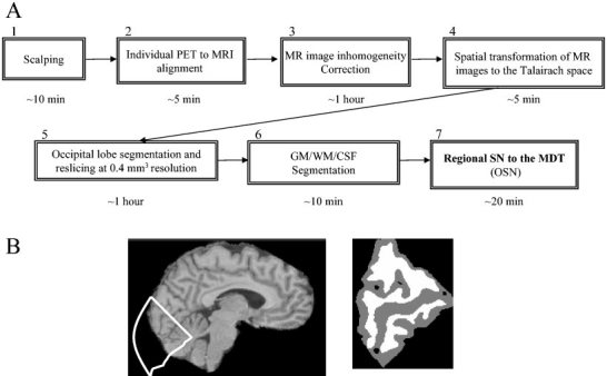
A: HRSN processing stream and the typical times per step. B: Examples of occipital lobe segmentation and OSN template building through WM/GM/CSF segmentation, which corresponds to steps 6 and 7.
Image preprocessing
An automated brain tissue segmentation procedure (BET) distributed as a part of the FSL package (http://www.fmrib.ox.ac.uk/fsl/) was used to remove the skull and non‐brain tissues (scalping) from anatomical MR images. The MR image intensity inhomogeneity was corrected using a bias field analysis method developed by Styner et al. [2000]. The subject's PET brain images were aligned and resliced to match the subject's anatomical image using an automated global spatial normalization software, Convex Hull (CH) [Lancaster et al., 1999] (online at http://ric.uthscsa.edu/projects). Next, CH was used for the global normalization of images by transforming them to the Talairach space.
Occipital lobe segmentation
Individual occipital lobes were manually segmented and resliced to build the OSN templates. An experienced neuro‐anatomist defined the occipital lobe using a 3‐D morphological software package, Display (MNI, online at http://www.bic.mni.mcgill.ca/), while viewing 1‐mm‐thick sagittal sections. The occipital‐cerebelar boundary was used as the ventral border (Fig. 1B). The occipito‐parietal border (Fig. 1B) was created by drawing a straight line through the parietal‐occipital (PO) fissure from its dorsal superficial surface to its ventral pit. Using a straight line, instead of tracing the PO fissure, simplified the segmentation process and reduced processing time. This occipital lobe segmentation consumed about 45 min per brain. Thirty slices from each hemisphere were extracted for each subject, resliced into 0.4 mm3 voxels and placed in the center of a 2563 space.
OSN template building
A fuzzy‐classifier anatomical segmentation method [Herndon et al., 1998] was used to segment images into white matter (WM), gray matter (GM), and cerebrospinal fluid (CSF). The automated segmentation was manually verified and corrected by a neuroanatomist. Anatomical templates [Kochunov et al., 2000] were created by magnitude coding of the tissue classes (WM, GM, and CSF).
Identifying and optimizing the target volume
A best individual target brain was identified based on the analysis of the deformation fields [Kochunov et al., 2001].
The MDT brain was obtained as follows:
-
1
The first image volume in the study was regionally spatially transformed with OSN to match all other volumes. Next, all volumes in the study were OSN warped to the first volume. The resulting deformation vector field (DVF) provided a set of vectors, pointing from a single voxel in the first volume to corresponding locations in the set of source brains and vice versa.
-
2
A set of DVFs that provided mapping from each image volume in the study to all other images was calculated [Kochunov et al., 2001].
-
3
The target quality scores (TQS) were calculated for each volume as a product of average displacement and dispersion distance. The volume with the lowest TQS was declared as an optimal target.
-
4
The average DVF for the optimal target was used to transform individual brain images into the minimal deformation configuration in the collective brain space [Kochunov et al., 2001].
Analysis
Reduction of anatomical variability
The reduction of anatomical variability following HRSN processing was quantified as the reduction in GM mismatch and the overlap of individual calcarine sulci. The GM boundary mismatch is calculated by counting the number of mismatched GM voxels (source volume voxel having a different tissue type from the target volume voxel) in the transformed source volume. The GM mismatch is a measure of the average regional fit quality. To assess specific regional match quality in the calcarine, the overlap for the calcarine sulcus among the brain image volumes in the study was calculated. Individual calcarine sulci in each hemisphere were manually identified and segmented into binary images for each of the brain image volumes in the study before and after HRSN processing. The overlap of individually defined calcarine sulci with the target brain's calcarine sulcus was determined.
Reduction of spatial variability of V1 horizontal meridian representation
Multisubject overlap and spatial variability of the activated areas in the calcarine sulcus was investigated before and after HRSN processing. The primary visual cortex, retinotopic area V1 (BA 17), is believed to have a strong structure‐function association with the calcarine sulcus. Most of the cytoarchitectonic studies [Amunds et al., 2000] and functional imaging experiments identify the calcarine sulcus as the anatomical landmark for the primary visual cortex, especially the horizontal meridian representation [DeYoe, et al., 1996 Horton and Hoyt 1991; Sereno et al., 1995]
The horizontal random dot (HRD) pattern was shown to produce very robust activations over a large part of the base of the calcarine sulcus [Hasnain et al., 1998], which simplified the identification task. The individual HRD activation maps representing task‐associated changes were obtained by subtracting the images acquired during the rest state from the images acquired during HRD state. This resulted in three subtraction images (one of each repetition of the HRD task) that were averaged and converted to the Z score maps [Fox et al., 1988]. Activation maps were thresholded at Z scores > 2.0 (P < 0.05) to insure statistical significance of selected activations.
PET images were acquired with a FWHM of ∼8 mm and were resliced at 1 mm to match the spacing in anatomical MR image. While all functional activations are expected to reside within GM, the low spatial resolution of the functional image and errors of PET to MR co‐registration can result in the mismatch between the centers of activation and its true anatomical sites. Individual anatomical images and the Z‐score maps were overlaid in the 3‐D image analysis tool (Medx, Sensor System). To constrain activation regions to the calcarine GM, only intersections between the proposed anatomical site (calcarine sulcus and adjacent gyral surfaces) and statistically significant activations (Z > 2.0) were considered. Right and left V1 areas were volumetrically identified and traced as contiguous clusters of activations that overlapped with the calcarine sulcus. Only datasets where activations were present in both left and right primary visual cortexes (9 out of 10) were used. The activation areas constrained to the calcarine GM were segmented from the functional image into a binary image. Centroids for individual left and right activations were calculated. Then images were transformed to the target's brain space using the individual's deformation field. The average centroid and spatial deviations were calculated for the images in the original and target brain spaces.
Improvements in the intersubject average maps
The effects of the HRSN processing were investigated by analyzing the difference between the intersubject average Z‐maps produced by the GSN and HRSN processing streams. For both processing streams, the individual subtraction images were calculated for HRD minus Rest conditions. The intersubject average Z‐score map for GSN processing was calculated by averaging the individual subtraction images and dividing by the voxel‐wise standard deviation. For the HRSN processing stream, the individual subtraction images for each subject were transformed into the target's space using individual deformation fields, then averaged and divided by voxel‐wise standard deviation.
The difference between the two processing streams was judged by analysis of the histogram of the activations found in the occipital lobe and by the histogram, size, and location of the presumed V1 horizontal meridian activation. The histogram of the occipital lobe activations is a global measurement of the alignment of individual functional areas, while measurement of V1 activations provides an insight to the regional alignment. For both GSN and HRSN processing streams, the activations of the horizontal meridian in the intersubject average image were analyzed by placing volumetric regions of interest that completely encompassed the activation site.
Statistically significant activations (Z > 2.0) in the vicinity of the calcarine sulcus were identified as the V1 horizontal meridian representation. The intersubject average HRD Z‐score map thresholded at Z = 2.0, was overlaid on the intersubject average anatomical image in a 3D image analysis tool (Medx, Sensor System). A single volumetric ROI was drawn for each hemisphere to encompass the site of the horizontal meridian using the calcarine sulcus anatomy as the reference. The mean activation, activation volume, location, and the histogram of the activation were collected for each region.
Results
Reduction of Anatomical Variability
The average GM mismatch was reduced from 38.7 ± 4.3% for GSN to 20.5 ± 3.4% following HRSN. This reduction clearly indicates a better registration of the bulk of the GM following HRSN processing. Analysis of the overlap frequency histogram for nine subjects (Fig. 2) shows that the average overlap frequency of voxels in individual calcarine sulci with the target's calcarine sulcus rose from 3.7 ± 1.8 following GSN to 6.8 ± 1.9. This is a significant improvement (two tailed χ2, P < 0.01) in the alignment between individual and target calcarine sulci following HRSN processing. The overlap frequency was slightly higher for the left hemisphere than for the right hemisphere, although this was not statistically different (two tailed P = 0.44).
Figure 2.
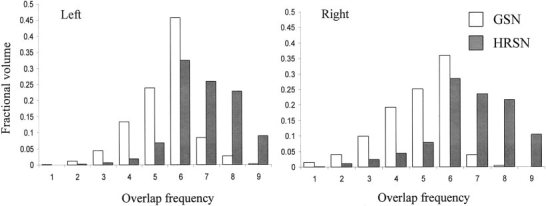
Calcarine sulci volume overlap frequency histogram for nine subjects following GSN and HRSN processing.
Intersubject Variability of V1 Horizontal Meridian
The horizontal meridian group overlap (Fig. 3, top row) shows considerable spatial spread, indicating a high intersubject variability of this structure following GSN. The HRSN processing significantly (two tailed χ2, P < 0.01) decreased the spread among individual areas (Fig. 3, bottom row) by improving registration between the individual calcarine structures and the target. The overlap frequency histogram for eight individual volumes (the target volume was excluded) was calculated for both anatomical and functional data (Fig. 4). The anatomical overlap histogram shows how many times a GM region labeled as “activated” overlapped with GM (both activated or not activated) of other subjects. The anatomical overlap histogram (Fig. 4A) shows that HRSN processing significantly improved the GM overlap among the subjects: the average gray matter overlap for activated voxels improved from 3.9 to 6.7 following HRSN. The functional overlap histogram also shows a great improvement following HRSN processing (Fig. 4B). Following GSN, only 5% of the activated voxels overlapped for two or more subjects. This number was improved by seven‐fold to 35% following HRSN. Also, the maximum number of overlapped individual areas increased from 4 to 6 and the mean overlap frequency increased from 1.5 to 2.2 (out of eight) overlapped areas per voxel.
Figure 3.
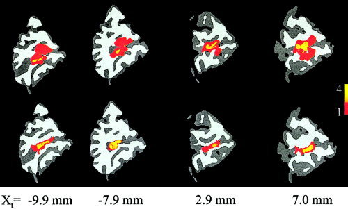
The color‐coded overlap among individual horizontal meridian (HM) V1 areas for eight subjects is shown on the target's sagittal slices, following GSN (top) and HRSN (bottom).
Figure 4.
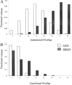
A: Anatomical overlap histograms: frequency of overlap among activated horizontal meridian (HM) GM voxels and calcarine GM. B: Functional overlap histogram: frequency of overlap among individual activated HM voxels.
The better overlap among individual areas observed in the overlap frequency histogram (Fig. 4) is also reflected in the reduction of the spatial deviation among the centroids of individual activated areas. The spatial deviation for each of the coordinates was reduced in all but x coordinate on the left side. The total spatial standard deviation of the individual centroids of activations was reduced from 5.3 mm following GSN to 3.8 mm following HRSN on the left and from 5.0 to 4.0 mm for the right retinotopic areas (Table I).
Table I.
HRD V1 activation overlap study.
| Site | x (mm) | y (mm) | z (mm) | Distance from the target |
|---|---|---|---|---|
| V1 activations, left calcarine sulcus | ||||
| Target | −7.3 | −79.2 | 3.5 | |
| GSN (mean) | −9.6 ± 2.5 | −78.3 ± 3.2 | 1.7 ± 3.4 | 3.0 |
| OSN (mean) | −9.6 ± 1.7 | −79.5 ± 3.0 | 2.5 ± 1.6 | 2.6 |
| V1 activations, right calcarine sulcus | ||||
| Target | 5.1 | −76.5 | 2.1 | |
| GSN (mean) | 5.9 ± 2.0 | −75.8 ± 3.4 | −2.0 ± 3.0 | 1.1 |
| OSN (mean) | 5.7 ± 2.1 | −75.6 ± 3.0 | 2.3 ± 1.7 | 1.1 |
The location for the average of individual centroids and distance from the target's centroid.
Improvements in the Intersubject Average Maps
The subtraction images between HRD and Rest states were isolated for comparison and spatially normalized using global and regional SN. The intersubject Z‐score maps were calculated for both conditions by dividing the intersubject average image by voxel‐wise standard deviation and thresholded at Z = 2.0 (P = 0. 0455). The Z‐score histograms of the whole occipital lobe (Fig. 5) show that HRSN processing produces more statistically significant activations and the peak of the histogram is shifted towards higher Z‐scores. Both of these trends indicate a better alignment among individual functional areas.
Figure 5.
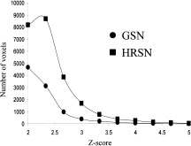
Z‐score histograms of activations due to horizontal random dot stimulus and after GSN and HRSN processing.
The activation volumetric ROI analyses (Table II) shows that the mean and maximum Z‐scores and the volume of activation are significantly higher following the HRSN processing. This is more obvious in the left horizontal meridian activation (HMA), which was essentially absent before (Table II). Following HRSN processing, the size and mean Z‐score values of the left HMA were not different from the right side activations. The normalized histograms of the right and left horizontal meridian Z‐scores show the shift of the peak of the histograms towards higher Z‐scores, indicating a better alignment of activations prior to intersubject averaging (Fig. 6).
Table II.
Regional Z‐score analysis for the V1 activation during HRD stimulus
| Site | x (mm) | y (mm) | z (mm) | Max Z score | Average Z score | Volume (mm3) |
|---|---|---|---|---|---|---|
| GSN | ||||||
| Left V1 | −13.9 | −79.5 | −0.5 | 2.4 | 2.0 ± 0.1 | 9.5 |
| Right V1 | 5.3 | −83.9 | 1.9 | 4.7 | 2.4 ± 0.5 | 102.3 |
| OSN | ||||||
| Left V1 | −12.3 | −77.9 | −2.9 | 5.6 | 2.5 ± 0.5 | 142.4 |
| Right V1 | 6.1 | −79.1 | 1.9 | 6.5 | 2.6 ± 0.6 | 144.9 |
Figure 6.
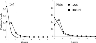
Left/right HM V1 Z‐score histograms following GSN and HRSN.
Conclusion and discussion
Measurement of Function‐Structure Correspondence
The existence of correspondence between individual retinotopic areas and anatomical structures was shown by studying histological slices [Amunts et al., 2000] and through imaging [Hasnain et al., 1998,2001]. This correspondence indicates that an advanced spatial normalization method, which significantly improves anatomical matching, would also improve the overlay of functional areas thus improving statistical confidence. The capability of HRSN to improve the anatomical alignment was studied using global (GM mismatch) and regional (calcarine sulcus overlap) features. Both studies indicated that HRSN processing resulted in a significant improvement in anatomical matching.
The first measure of a structure‐function relationship was the improved overlap of the horizontal meridian activated areas of the calcarine sulcus during the HRD stimulus following GSN and HRSN processing. By artificially confining activations to their anatomical landmark (calcarine sulcus), more detailed analyses were made possible. First, by linking functional and anatomical areas through a “cookie cutting” strategy (cutting functional data using the anatomical data as a template), the reduction of functional variability can be studied in the case of ideal PET/MR registration. Second, since only the intersection between statistically significant (Z > 2.0) activations and the calcarine sulcus was considered, the apparent spatial resolution of the functional data was artificially enhanced, e.g., the artifacts of interpolating functional data from 8 to 1 mm resolution were eliminated.
The colored overlays (Fig. 3) show that following GSN there is a registration failure: the activations residing on the individual's calcarine sulcus are mapped to the 1st dorsal (Fig. 3, x = −9.9, −7.9 mm, top row) or 2nd ventral (Fig. 3, x = 2.9, 7.0 mm, top row) sulcus of the target brain. This misalignment was resolved by HRSN processing, with all the calcarine activations mapped to the target's calcarine sulcus (Fig. 3, right column). The penetrance image (Fig. 3) also visualizes an improvement in the registration of individual functional areas and the overlap histogram (Fig. 4) gives a quantitative measure of improvement. The most significant change, following HRSN, in the overlap histograms (Fig. 4) is seen for the areas that overlapped at least once. While, the volume of non‐overlapping areas was reduced by 10%, following HRSN, the volume of areas that overlapped once was reduced by 20%, the volume of areas that overlapped three times was increased by 19%, and the volume of areas that overlapped four times was increased by 9%.
Intra‐Calcarine Variability of HMA
The above results can be interpreted such that while HRSN significantly improved functional registration by matching sulci, there still exists a variability that HRSN processing does not account for. The anatomical overlap histogram (Fig. 4B) shows that the majority of the activated GM overlapped with at least 4 other subject's GM following HRSN. The unaccounted variability is believed to be the variability of individual areas within the calcarine sulcus, which cannot be resolved by HRSN. This conclusion is supported by the measurement of variability of the centroids of the individual activations. The spatial variability along each direction was reduced in all but one case (did not change for x direction of the left hemisphere). The spatial variability along x and z was lower than along the y direction. The OSN fitting cost function is derived to maximize the overlap among tissues of the same type, thus the deformation in this region is calculated to overlap the source and target's calcarine sulci. Since maximal overlap requires mostly deformations along x (right‐to‐left) and z (dorsal‐to‐ventral), lower variability is expected. The variability along y, which roughly corresponds to the direction along the calcarine sulcus, remains the highest for both left and right hemispheres.
We reported intra‐calcarine variability of HMA in our previous analysis [Hasnain et al., 2001]. In general, the surface length of the calcarine is oriented along the anterior‐posterior (y‐) axis. Of the 11 individuals in our study, 9 had the center of the right HMA located within the calcarine sulcus. In terms of the anterior‐posterior axis (y‐axis), six out of nine subjects had the centeroid of right HMA halfway up the length of the calcarine sulcus from the occipital pole. Out of the remaining three subjects, one had the right HMA centeroid one‐third way up the length of the calcarine sulcus, and two had it one‐quarter way up from the occipital pole. Similarly, in the left hemisphere the center of left HMA activation was located one‐fourth way up the length of the calcarine sulcus in two individuals, one‐third way up in five individuals, half‐way up the length of the calcarine in three subjects, and two‐thirds way up the length of the calcarine in one subject. Although there was variability of HMA with respect to the fundus (medio‐lateral or x‐axis) and the shoulders (superior‐inferior or z‐axis) of the calcarine, this was less in magnitude.
Clearly, the source of intra‐sulcal variability of HMA is at least partially genetic. Several genes whose expression defines regional boundaries in the developing cerebral cortex have recently been described. For example, Rubenstein et al. [1999] present evidence that expression patterns of Id‐2, Tbr‐1, cadherin‐6, cadherin‐8, neuropilin‐2, Wnt‐7b, Eph‐A7, and RZR‐beta have regional boundaries that demarcate distinct functional areas of the cerebral cortex in neonatal mice. These genes, some of which are expressed in gradients, and others in discrete domains, are likely candidates for regulating cytoarchitectonic topography and functional anatomy [Rubenstein and Rakic, 1999].
In our recent article [Hasnain et al., 2001], we hypothesized that the timing of formation is important in determining whether a sulcus will spatially co‐vary with functional architecture. Formation of the primary sulci in mammals occurs during the second trimester, as neurons migrate along glial radials from the ventricular proliferative centers to the cortical surface [Rakic and Singer, 1988]. These are predominantly glutamate‐ergic pyramidal neurons [Corbin et al., 2001]. During this stage of radial growth of the cerebral cortex, the topography of the functional map is strongly influenced by the genetically determined ventricular functional proto‐map. The development of sulci and functional areas may be tightly linked during this stage, as witnessed by the relatively constant relationship between primary sulci and functional areas that form during this period.
By the beginning of the third trimester, the radial neuronal migration is complete. During the third trimester and for some time after birth, the cortical development is predominated by the maturation of the neuropil [Berry, 1982] and intra‐cortical connections. Moreover, neurons may migrate tangentially at these later stages of corticogenesis [Rakic, 1990]. GABA‐ergic interneurons originating from the lateral ganglionic eminence migrate tangentially during the third trimester [Anderson et al., 2001]. Hence, tangential growth of the cerebral cortex continues after radial migration of neurons is completed. The differential tangent growth of outer cortical lamina when compared with the inner cortical layers as postulated by Richman et al., [1975] must occur at these later stages because the outer layers are the last to form during radial migration of neurons. Therefore, the formation of secondary and tertiary sulci during the third trimester and during the immediate postnatal period may be more influenced by simple mechanical folding of the cortex. This more or less random buckling as well as formation of intra‐cortical connections may actually distort and displace the original placement of the functional areas and would partially account for the non‐genetic component of intra‐calcarine variability of HMA.
Reduction of Spatial Variance as a Measure of Sulcal‐Functional Co‐Variance
HRSN processing improves group statistical significance of functional areas with strong function‐anatomy association and the degree of improvement may serve as a measure of the strength of sulcal‐functional co‐variance in a given brain region. In our data, the level of improvement was the most significant for the HMA of the left hemisphere. This activation (Table II) was essentially absent following GSN processing. Following HRSN processing, the activation volume and average Z‐score were symmetric between hemispheres, i.e., the activation volume and average Z‐scores were not different for both hemispheres. The higher degree of improvement in group statistical significance of functional areas in the left hemisphere was predicted by our previous results [Hasnain et al., 2001]. More sulcal‐functional co‐variance were found in the left hemisphere and these co‐variances were generally stronger than those found in the right hemisphere. Such inter‐hemispheric asymmetries of sulcal patterns and functional areas are well documented. These reports [Lohmann et al., 1999 Tramo et al., 1995]; show a lower degree of variability in surface size for the left hemisphere and a stronger genetic influence on the sulcal shape and size of several cortical surface areas in the left hemisphere when compared to the right hemisphere.
These data show that high‐resolution regional spatial normalization can be used to improve statistical significance of intersubject activations in the primary visual areas. This potentially offers an alternative to extensive spatial filtering of the data in order to improve intersubject overlap. Improvement will only be seen in the area with significant structure‐functional covariance since cross‐subject alignment is driven by anatomical features. HRSN is an efficient automated method to investigate the spatial relationship between function and anatomy as opposed to labor‐intensive measurements of spatial covariance. We are in the processing of developing a technique to calculate structure‐functional spatial covariance based on the amount of improvement of the statistical significance and reduction in spatial extend following HRSN processing.
Future Developments
We plan to perform similar studies in other areas with well‐established structure‐functional covariance such as the M1 area of the motor cortex and hypothalamus nuclei. Also, we plan to apply this method to study structure‐functional relation with a disputed structure‐functional association such as planum temporale and Herche gyrus, with the hope of finding a definite answer.
Another potentially important application of HRSN could be its use in conjunction with cortical‐flattening techniques [Dale et al., 1999, Van Essen et al., 2001]. Cortical flattening techniques allow for simpler identification and better visual representation of activated areas by placing activations on a flattened map. Two major drawbacks of these techniques are: inability to perform intersubject averaging and the time and manual effort needed to perform the flattening of each brain. We believe that HRSN can be used to remedy both of these problems. HRSN can be used to warp individual images to the target for which the flattening transformation was previously established. Thus, the individual functional images can be averaged in 3‐D space and then overlaid on the flattened cortical surface for further analysis and visual presentation.
Acknowledgements
Research support was provided by the Human Brain Mapping Project, which is jointly funded by National Institute of Mental Health and National Institute on Drug Abuse (P20 MH/DA52176).
REFERENCES
- Amunts K, Malikovic A, Mohlberg H, Schormann T, Zilles K (2000): Brodmann's areas 17 and 18 brought into stereotaxic space‐where and how variable? Neuroimage 11: 66–84. [DOI] [PubMed] [Google Scholar]
- Anderson SA, Marin O, Horn C, Jennings K, Rubenstein JL (2001): Distinct cortical migrations from medial and lateral ganglionic eminences. Development 128: 353–563. [DOI] [PubMed] [Google Scholar]
- Armstrong E, Curtis M, Buxhoeveden DP, Fregoe C, Zilles K, Casanova MF, McCarthy WF (1991): Cortical gyrification in the Rhesus monkey: a test of the mechanical folding hypothesis. Cerebral Cortex 1: 426–432. [DOI] [PubMed] [Google Scholar]
- Armstrong E, Schleicher A, Omran H, Curtis M, Zilles K (1995): The ontogeny of human gyrification. Cerebral Cortex 5: 56–63. [DOI] [PubMed] [Google Scholar]
- Berry M (1982): Cellular differentiation: Development of dendritic arborizations under normal and experimentally altered conditions. Neurosci Res Prog Bull 20: 451–461. [PubMed] [Google Scholar]
- Collins D, Neelin P, Peters Y, Evans A (1994): Automatic 3D intersubject registration of MR volumetric data in standardized space. J Comput Assist Tomogr 18: 192–205. [PubMed] [Google Scholar]
- Collins D, Holmes C, Peters T, Evans A (1995): Automatic 3‐D model‐based neuroanatomical segmentation. Hum Brain Mapp 3: 190–208. [Google Scholar]
- Corbin JG, Nery S, Fishell G (2001): Telencephalic cells take a tangent: non‐radial migration in the mammalian forebrain. Nature Neurosci 4(Suppl) 1177–1182. [DOI] [PubMed] [Google Scholar]
- Dale A, Fischl B, Sereno M (1999): Cortical surface‐based analysis. I. Segmentation and surface reconstruction. Neuroimage 9: 179–94. [DOI] [PubMed] [Google Scholar]
- DeYoe EA, Carman GJ, Bandettini P, Glickman S, Wieser J, Cox R, Miller D, Neitz J (1996): Mapping striate and extrastriate visual areas in human cerebral cortex. Proc Natl Acad Sci U S A 93: 2382–2386. [DOI] [PMC free article] [PubMed] [Google Scholar]
- Fox PT, Mintun MA, Raichle ME, Miezin FM, Allman JM, Van Essen DC (1986): Mapping human visual cortex with positron emission tomography. Nature (Lond) 323: 806–809. [DOI] [PubMed] [Google Scholar]
- Fox PT, Mintun MA, Reiman EM, Raichle ME (1998). Enhanced detection of focal brain responses using intersubject averaging and change‐distribution analysis of subtracted PET images. J Cereb Blood Flow Metab 1988 Oct;8(5): 642–653. [DOI] [PubMed] [Google Scholar]
- Fox PT, Raichle M (1985): Stimulus rate determines regional blood flow in striate cortex demonstrated by positron emission tomography. Ann Neurol 17: 303–305. [DOI] [PubMed] [Google Scholar]
- Fox PT, Miezen FM, Allman JM, Van Essen DC, Raichle ME (1987): Retinotopic organization of human visual cortex mapped with positron emission tomography. J Neurosci 7: 913–922. [DOI] [PMC free article] [PubMed] [Google Scholar]
- Fox PT (1995): Spatial normalization origins: objectives, applications, and alternatives. Hum Brain Mapp 3: 161–164. [Google Scholar]
- Hasnain MK, Fox PT, Woldorff MG (1998): Intersubject variability of functional areas in the human visual cortex. Hum Brain Mapp 6: 301–315. [DOI] [PMC free article] [PubMed] [Google Scholar]
- Hasnain MK, Fox PT, Woldorff MG (2001): Structure‐function spatial covariance in the human visual cortex. Cerebral Cortex 11: 702–16. [DOI] [PubMed] [Google Scholar]
- Horton JC, Hoyt WF (1991): The representation of the visual field in human striate cortex. A revision of the classic Holmes map. Arch Ophthalmol 109: 816–824. [DOI] [PubMed] [Google Scholar]
- Kochunov P, Lancaster J, Fox PT (1999): Accurate high‐speed spatial normalization using an octree method. NeuroImage 10: 724–737. [DOI] [PubMed] [Google Scholar]
- Kochunov P, Lancaster J, Thompson P, Boyer A, Hardies J, Fox PT (2000): Validation of octree regional spatial normalization method for regional anatomical matching. Hum Brain Mapp 11: 193–206. [DOI] [PMC free article] [PubMed] [Google Scholar]
- Kochunov P, Lancaster J, Thompson P, Woods R, Fox PT (2001): Regional spatial normalization: towards the optimal target. J Comput Assist Tomogr 25: 805–816. [DOI] [PubMed] [Google Scholar]
- Kochunov P, Lancaster J, Thompson P, Toga A, Brewer P, Hardies J, Fox PT (2002): An optimized individual target brain in the Talairach coordinate system, Neuroimage 17: 922. [PubMed] [Google Scholar]
- Lancaster J, Fox P, Downs H, Nickerson D, Hander T, Mallah M, Zamarripa F (1999): Global spatial normalization of the human brain using convex hulls. J Nuclear Med 40: 942–955. [PubMed] [Google Scholar]
- Lancaster JL, Woldorff MG, Parsons LM, Liotti M, Freitas CS, Rainey L, Kochunov PV, Nickerson D, Mikiten SA, Fox PT (2000): Automated Talairach atlas labels for functional brain mapping. Hum Brain Mapp 10: 120–131. [DOI] [PMC free article] [PubMed] [Google Scholar]
- Lohmann G, Cramon DYV, Steinmetz H (1999): Sulcal variability of twins. Cerebral Cortex 9: 754–763. [DOI] [PubMed] [Google Scholar]
- Rakic P, Singer W (1988): Neurobiology of the neocortex. New York: John Wiley and Sons. [Google Scholar]
- Rakic P (1990): Principles of neural cell migration. Experientia 46: 882–891. [DOI] [PubMed] [Google Scholar]
- Richman DP, Stewart RM, Hutchinson JW, Caviness VS Jr ( 1975): Mechanical model of brain convolutional development. Science 189: 18–21. [DOI] [PubMed] [Google Scholar]
- Rubenstein JLR, Rakic P (1999): Genetic control of cortical development. Cerebral Cortex 9: 521–523. [DOI] [PubMed] [Google Scholar]
- Rubenstein JLR, Anderson S, Shi L, Miyashita‐Lin E, Bulfone A, Hevner R (1999): Genetic control of cortical regionalization and connectivity. Cerebral Cortex 9: 524–532. [DOI] [PubMed] [Google Scholar]
- Sereno MI, Dale AM, Reppas JB, Kwong KK, Belliveau JW, Brady TJ, Rosen BR, Tootell RB (1995): Borders of multiple visual areas in humans revealed by functional magnetic resonance imaging. Science 268: 889–893. [DOI] [PubMed] [Google Scholar]
- Smart IHM and Mc Sherry GM (1986): Gyrus formation in the cerebral cortex of the ferret. II. Description of the internal histological changes. J Anat 147: 27–43. [PMC free article] [PubMed] [Google Scholar]
- Styner M, Brechbuhler C, Szekely G, Gerig G (2000): Parametric estimate of intensity inhomogeneities applied to MRI. IEEE Trans Med Imaging 19: 153–165. [DOI] [PubMed] [Google Scholar]
- Tramo MJ, Loftus WC, Thomas CE, Gazzaniga MS (1995): Surface area of human cerebral cortex and its gross morphological subdivisions: in vivo measurements in monozygotic twins suggest differential hemisphere effects of genetic factors. J Cogn Neurosci 7: 292–301. [DOI] [PubMed] [Google Scholar]
- Van Essen DC (1997): A tension‐based theory of morphogenesis and compact wiring in the central nervous system. Nature 385: 313–318. [DOI] [PubMed] [Google Scholar]
- Van Essen DC, Drury HA, Dickson J, Harwell J, Hanlon D, Anderson CH (2001): An integrated software suite for surface‐based analyses of cerebral cortex. J Am Med Info Assoc 8: 443–459. [DOI] [PMC free article] [PubMed] [Google Scholar]
- Welker W (1990). Why does cerebral cortex fissure and fold? A review of determinants of gyri and sulci In: Jones EG, Peters A, editors. Cerebral cortex, vol 8B 3–136. New York: Plenum. p 3–136. [Google Scholar]
- White T, O'Leary D, Magnotta V, Arndt S, Flaum M, Andreason N (2001): ). Anatomic and functional variability: the effect of the filter size in group fMRI data analysis. Neuroimage 13: 577–588. [DOI] [PubMed] [Google Scholar]