Robust estimation of the probabilities of 3‐D clusters in functional brain images: Application to PET data

Abstract

Recently, we presented a method (the CS method) for estimating the probability distributions of the sizes of supra threshold clusters in functional brain images [Ledberg A, Åkerman S, Roland PE. 1998. Estimating the significance of 3D clusters in functional brain images. NeuroImage 8:113–128]. In that method, the significance of the observed test statistic (cluster size) is assessed by comparing it with a sample of the test statistic obtained from simulated statistical images (SSIs). These images are generated to have the same spatial autocorrelation as the observed statistical image (t‐image) would have under the null hypothesis. The CS method relies on the assumptions that the t‐images are stationary and that they can be transformed to have a normal distribution. These assumptions are not always valid, and thus limit the applicability of the method. The purpose of this paper is to present a modification of the previous method, that does not depend on these assumptions. This modified CS method (MCS) uses the residuals in the linear model as a model of a dataset obtained under the null hypothesis. Subsequently, datasets with the same distribution as the residuals are generated, and from these datasets the SSIs are derived. These SSIs are t‐distributed. Thus, a conversion to normal distribution is no longer needed. Furthermore, no assumptions concerning the stationarity of the statistical images are needed. The MCS method is validated on both synthetical images and PET images and is shown to give accurate estimates of the probability distribution of the cluster size statistic. Hum. Brain Mapping 9:143–155, 2000. © 2000 Wiley‐Liss, Inc.

INTRODUCTION

The detection of regional changes in tissue blood flow and blood oxygenation level is one of the main goals of functional brain imaging. This goal is often accomplished in two steps: In the first step, a linear model is fitted to each and every voxel. Then, hypotheses are tested on the fitted parameters. Each tested hypothesis results in a statistical image (SI). These images are usually so called t‐images, where the “t” refers to the fact that the obtained statistics (one for each voxel) are distributed as Student's t. In the second step, the purpose is to decide which regional changes in the SIs are “true” changes and which are the result of random fluctuations. This way of analyzing functional brain imaging data was introduced by Friston and colleagues [Friston et al., 1990, 1991] and is usually referred to as statistical parametric mapping. To find the “true” changes, one usually derives a test statistic from the SI (e.g., global maximum or cluster size) and then compares the value of this statistic with values of the same statistic obtained under the null hypothesis. However, the exact probability distributions (pds) of these statistics are usually unknown, even under the assumption that the data is normally distributed. One therefore has to resort to some kind of estimation of the pd. This is a problem faced by all existing methods of statistical analysis of functional imaging data. Furthermore, the way in which this estimation is made constitutes the main differences between the different methods. One commonly used approach is to estimate the smoothness of the SI and then to use results from random field theory to obtain expressions for the pds of the different statistics: global maxima [Worsley et al., 1992, 1996] and cluster size (for Gaussian SI) [Friston et al., 1994; for a review, see Cao, 1997]. Recent developments in this field have enabled an approximate expression for the pd of cluster sizes also for t‐images [Cao, 1997, 1999]. For a stationary t‐image, this expression only is dependent on the smoothness and the degrees of freedom (df) of the t‐image. However, since the smoothness usually is unknown, it has to be estimated, and the pds of the test statistics are dependent on this estimate. Another approach to obtain probabilities of different test statistics is the nonparametric method described in Holmes et al. [1996]. Here, a randomization approach is used to test hypotheses on the test statistics, and this approach is basically free from assumptions.

The fact that the pd of the test statistic is dependent on parameters that are difficult to estimate makes the statistical analysis of functional imaging data different from the traditional usage of statistical tests where the pd of the test statistic is known and often even tabulated. It is therefore an important task to find good estimators of the pd of test statistics in functional brain image analysis.

In a recent paper, we described a method (referred to as the CS method) that can be used to estimate the pd of cluster sizes [Ledberg et al., 1998]. This method utilizes a linear model to test hypotheses and thus to generate SIs (t‐images). These images are subsequently converted to normal distributed images (i.e., Gaussianized). The cluster size (i.e., the number of connected voxels above a certain threshold) is the statistic used to detect the regional changes. The pd of this statistic is estimated with Monte Carlo simulations. In these simulations, a large number of random images (referred to as simulated statistical images, SSIs) are generated to represent SIs under the null hypothesis. These simulations are based on the assumption that the Gaussianized t‐images can be approximated by stationary normally distributed images. This is a good approximation for t‐images with many degrees of freedom but is less good for t‐images with few df and thus limits the usage of the CS method. Furthermore, the approach adopted to generate the SSIs, although technically correct is difficult to implement due to the relatively small size (i.e., number of voxels in each dimension) of the images, especially when the images are heavily smoothed.

The purpose of the present paper is to present a more robust method for generating the pd of the cluster size statistic under the null hypothesis. This method requires the statistical images to be neither normally distributed nor stationary. The main steps of the proposed method are: (i) fitting a linear model to the data, (ii) testing hypotheses on the parameters in the model, (iii) generating many SSIs having the same pd as the observed SI would have under the null hypothesis, and (iv) searching these generated SSIs for clusters above a certain threshold in order to estimate the pd of the cluster size statistic. The difference between this modified CS method (henceforth MCS method) and the CS method of Ledberg et al. [1998] concerns the generation of the SSIs (i.e., step iii). The SSIs are now generated from datasets having the same distribution as the residuals in the linear model. The variates in each and every voxel of these SSIs are t‐distributed; thus, the original t‐image need not be Gaussianized. Furthermore, the SIs need not be stationary for this approach to be applicable. Detailed descriptions of each step is given in the next section. The method is validated on two different sets of images: synthetical and real PET images. A comparison between the MCS and the CS method also is made. The validation shows that the MCS method gives reliable estimates of the pds, and the comparison with the CS method shows that the MCS method is indeed a significant improvement of the CS method.

THEORY

Notation

Let the following boldface upper case letters denote matrices and boldface lower case letters denote vectors. Sometimes, where appropriate, vectors will be referred to as images and the components of the vectors as voxels of the image. Let A′ denote the transpose of A, let A ⁻ denote a generalized inverse of A. Let ⊗ denote the Kronecker product. Let N(M, Φ_n ⊗ Σ_v) represent the multivariate normal distribution with mean value matrix M and covariance matrix Φ_n ⊗ Σ_v, where Φ_n is a symmetric nonnegative definite n ×n matrix and Σ_v is a symmetric nonnegative definite v ×v matrix. This notation means that if U = (u₁u₂ ⋮ u_n)′ is a n ×v random matrix, then to say that U is distributed as N(M, Φ_n ⊗ Σ_v) means that the nv × 1 vector (u₁, u₂, ⋮, u_n)′ is normally distributed with mean vector (m₁, m₂, ⋮, m_n)′ and covariance matrix Φ_n ⊗ Σ_v, where m_iis the ith row of the n ×v matrix M. Let t _r represent the univariate Student's t distribution with r df. An image in which the variables in each and every voxels are distributed as t _r is called a t‐image and the values in the voxels in this image are called t‐values. With the df of a t‐image is meant the df of the t‐distributed values in each voxel. Let diag(A) be a matrix operation that sets all the off diagonal terms of A to zero. Finally some notation concerning clusters. If t is a t‐image with a certain df, let clu(t, α) denote the sets of connected voxels in t in which all voxels have a t‐value equal to or higher than the t‐value corresponding to a p‐value of α. Note that this t‐value is dependent on the df of the image. For example, if t has 53 df and α = 0.01 then clu(t, α) are the sets of connected voxels in t in which all voxels have a t‐value equal to or higher than 2.399. α and the corresponding t‐value will be referred to as the “threshold” of t interchangeably. These sets of connected voxels are called “clusters,” and the size of a cluster is the number of voxels it consists of. Let s(clu(t, α)) denote the set of sizes of the clusters in t above the threshold α and let max{s(clu(t, α))} denote the maximum of these sizes.

Fitting a Linear Model to the Data

Consider a set of functional images obtained in a number of subjects. As an example take six subjects, ten scans per subject, five obtained under the condition TEST and five under CONTROL. All images are assumed to be in the same anatomical format so that voxel‐wise comparisons make sense. Let Y be a n ×v matrix where n is the number of scans (i.e., 60 in the example) and v is the number of voxels in each scan. That is, each scan is represented as a row in Y. Let X be a n ×p design matrix; thus, there are p parameters in the model. A linear model for the data is then

(1)

Here B is a p ×v matrix that contains the parameters for each voxel and E is a n ×v matrix of error terms. The df of this model is γ =n − rank (X). This model is equivalent to the design model described in Ledberg et al. [1998] but formulated for all voxels at the same time. Figure 1 shows the design matrix for the example case. Only two factors, condition (two levels) and subject (six levels), are used in this case. Let B̂ be the matrix containing the parameter estimates (i.e., B̂ = (X′X)⁻ X′Y) and let R = Y − XB̂ be the matrix containing the residuals. To proceed, the following assumption is needed: E is distributed as N(0, I_n ⊗ Σ;) and rank (Σ) =v.

Figure 1.

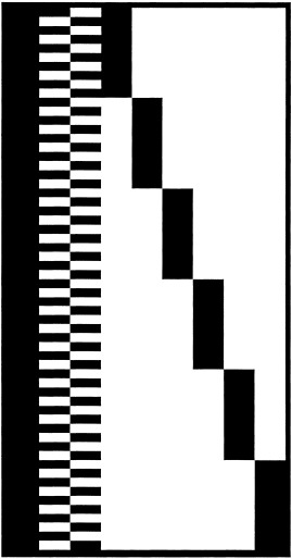
This figure shows the design matrix used. The columns refer to mean value (one column), task factor (two columns) and subject factor (six columns). The rows represents the scans.

Testing Hypotheses on the Estimated Parameters

Almost all hypotheses of interest can be formulated as linear combinations of the estimated parameters, so called contrasts. In the example, consider the contrast TEST‐CONTROL. That contrast would be implemented by hB̂, with h = [0 1 −1 0 0 0 0 0 0]. The variance of this contrast can be estimated as varˆ(hB̂) = diag{R′R(h(X′X)⁻ h′)}/γ [Graybill, 1976; Muirhead, 1982]. If hB̂ is divided with the square root of this estimated variance we get a SI t say,

(2)

Such a SI is referred to as a t‐image, because the variable in each and every voxel is distributed as t _γ.

To detect the significant regional changes in t, s(clu(t, α)) is compared to the pd of max{s(clu(t _null, α))} where t _null denotes a t‐image obtained under the null hypothesis. A cluster of size s is classified as significant at the 0.05 level if

(3)

The next issue then concerns how to estimate the pd of max{s(clu(t _null α))}. This pd will be estimated by generating many images having the same pd as t would have had under the null hypothesis and sampling these simulated t‐images for the largest clusters. How these SSIs are generated is the issue of the next section.

Generating the Images

This is the most important step in the MCS method and is also the step where the MCS method differs from the CS method. The generation of the images is based on a very simple idea described below. Some of the more technical aspects are dealt with in the Appendix.

The main idea is to generate a set of images having the same distribution as the real images would have under the null hypothesis and then to derive a t‐image from these images. The original data matrix Y should not be a realization of the null hypothesis (because there should be differences between TEST and CONTROL). Instead, the residuals R will be used as a model for a dataset obtained under the null hypothesis. This is intuitively appealing since if B = 0 in the linear model (Eq. 1), then R ≃ Y. The issue is then to generate datasets having the same distribution as R. To do this, one can use the fact that distributions of the type N(0, I_n ⊗ Σ) are invariant under left multiplication with orthogonal matrices [i.e., if Z is distributed as N(0, I_n ⊗ Σ)] and Γ is an orthogonal n ×n matrix then ΓZ will also be distributed as N(0, I_n ⊗ Σ). However, the situation is slightly more complicated since R is distributed as N(0, M ⊗ Σ) where M = (I − X(X′X)⁻ X′), so it has to be transformed into a distribution of the N(0, I_n ⊗ Σ) type for the invariance argument to work. How this can be done is shown in the Appendix. Thus, a matrix, R̃ say, distributed as N(0, I_γ ⊗ Σ) is generated. From this matrix, new matrices, R_i say, with the same distribution, are derived as follows: R̃_i= Γ_iR̃ where Γ_i is a random orthogonal matrix of size γ × γ. From these R̃_i images, t‐images are generated by, for each column, dividing the estimated mean value with the estimated standard deviation. This will generate a t‐image with γ − 1 df.

Estimating the Probability Distribution

The df of the simulated t‐images generated as described above, is γ − 1, whereas the df of the original t‐images is γ. However, by using thresholds corresponding to the same α, this discrepancy should not matter. Thus, each of the simulated t‐images is searched for clusters above the threshold given by α at γ − 1 df, whereas the real t‐images are searched for clusters above the threshold given by α at γ df. The estimation of the pd of max{s(clu(t, α))} from the simulated t‐images is done as follows: the probability of obtaining a cluster of size s say, is estimated by dividing the number of simulated t‐images in which a cluster of size s or larger occurred with the total number of simulated t‐images [see Eq. 11 in Ledberg et al., 1998].

VALIDATION

In this section, the MCS method is validated and compared to the CS method. This validation/comparison is made on two different sets of data. The first set consists of synthetical (i.e., computer‐generated) noise images, and the second set consists of real PET data. Because the true pd of the cluster size statistic is unknown, the validity of the pd estimated with MCS method will be investigated by a comparison with a reference pd derived by a randomization procedure. The choice of reference pd is important, and is the issue of the next section.

Generating the Reference Distribution

To see whether the MCS method gives an accurate estimation of the pd of the cluster size statistic, one would like to know the true distribution. Because this distribution is unknown, it also needs to be estimated by some means. I have chosen to use a nonparametric randomization procedure to derive the reference distribution. A randomization procedure is not dependent on any strong assumptions about the data (assumptions that might be wrong) and is in this respect, a good way to generate the reference distribution. A general introduction to randomization tests is given in Edgington [1980], and for an applications to PET images, see Holmes et al. [1996] and Ledberg et al. [1998].¹ As argued in Ledberg et al. [1998], a randomization procedure might lead to conservative estimates of the pd of the cluster size statistic. This is because some of the randomizations will be close to the original ordering of the scans, and thus the derived t‐image will contain signal. One way around this problem is to use a step‐down procedure [Holmes et al., 1996]. In the step‐down procedure, one starts with a randomization on the whole image (the first step). The voxels belonging to significant clusters (if any) are then removed and a new set of randomizations is performed on the remaining voxels (the second step). The significant clusters (if any) are again removed and a new set of randomizations are performed (the third step). In principle, one can continue as long as there are any significant clusters in the original t‐image.

Synthetical Images

Three different sets of synthetical images of size 64 × 64 × 64 voxels were generated, with the value of each voxel distributed as N(0, 1). The images in the first set were smoothed with a Gaussian kernel of three voxels FWHM and those in the second set with a kernel of six voxels FWHM. The images in the third set were smoothed with a Gaussian kernel of three voxels FWHM in the central part and with a kernel of six voxels FWHM in the peripheral parts. The purpose of using two filters of different widths in the same image was to generate nonstationary images (Fig. 2). To the first two sets of images, three linear models of 14, 30, and 62 df, respectively, were applied. For each combination of smoothness and df, the pd of the cluster size statistic at two different thresholds was determined with the MCS method using 5000 SSIs. The reference distribution was calculated by the randomization procedure. The results are shown in Figures 3 and 4. Because in this case there are no signals in the images, the randomizations will give the correct distribution without using the step‐down approach. However, for low df, only very few randomizations can be made, which makes the estimates noisy (as can be seen in the figures). It is clear from the figures that the MCS method gives accurate estimates for p‐values above 0.01 for both filter widths and all df. For smaller p‐values, the lack of fit between the MCS and the randomization method is probably because of the low number of randomizations used. This is because estimating the tails of the pd requires many simulations/randomizations. To verify that the two estimates do converge, a large number of simulations/randomizations were made on a set of smaller images. These images were the central 39 × 39 × 39 voxels of the images comprising the three voxel FWHM dataset. 15000 simulations/randomizations were made on these images with a model of 62 df. The results are shown in Figure 5. It is clear that the two estimates are very similar if enough simulations/randomizations are made.

Figure 2.

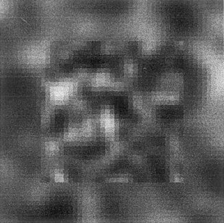
This figure shows a section from one of the nonstationary images used in the validation. The central part was filtered with a Gaussian filter with three voxels FWHM and the peripheral part with a Gaussian filter with six voxels FWHM.

Figure 3.

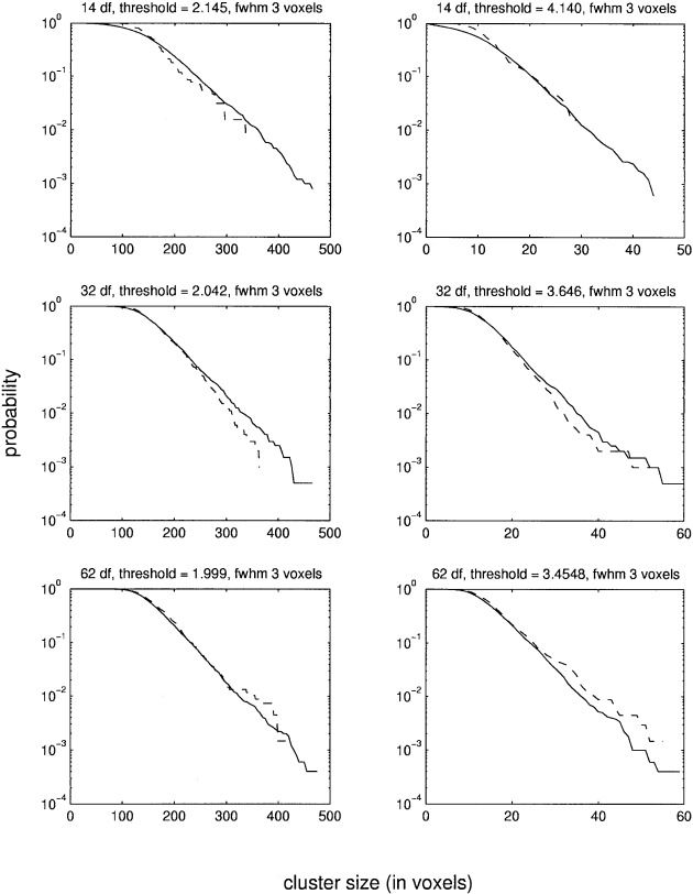
This figure shows the estimated probabilities of the cluster size statistic. The data are from the synthetical images filtered with a Gaussian filter of three voxels FWHM. Two different thresholds were used for each df. The dashed line shows the reference distribution as determined by randomizations. The solid line shows the probabilities estimated with MCS method. Please note that a logarithmic scale is used for the y‐axis.

Figure 4.

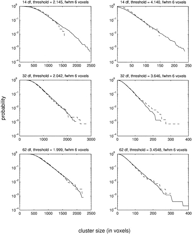
This figure shows the estimated probabilities of the cluster size statistic. The data are from the synthetical images filtered with a Gaussian filter of six voxels FWHM. Two different thresholds were used for each df. The dashed line shows the reference distribution as determined by randomizations. The solid line shows the probabilities estimated with the MCS method. Please note that a logarithmic scale is used for the y‐axis.

Figure 5.

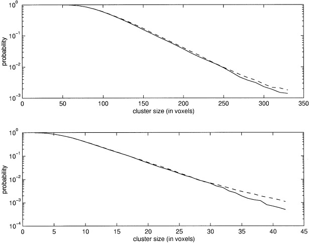
This figure shows the estimated probabilities of the cluster size statistic on a subset of the three voxel FWHM dataset. 15,000 simulations/randomization were made. The solid and dashed lines refer to the MCS and randomization methods, respectively. The top figure shows cluster sizes above a threshold of 2.0 and the lower figure above thresholds of 3.457 and 3.454 for the MCS and randomization methods, respectively.

For the third set of images, the nonstationary set, a model of 62 df was applied. The pd of the cluster size statistic was estimated with the MCS method as well as with the CS method. The reference distribution was calculated with the randomization procedure. The result is shown in Figure 6. It is clear that the MCS method gives very accurate estimates also on these nonstationary images. However, the CS method performed less well, as expected.

Figure 6.

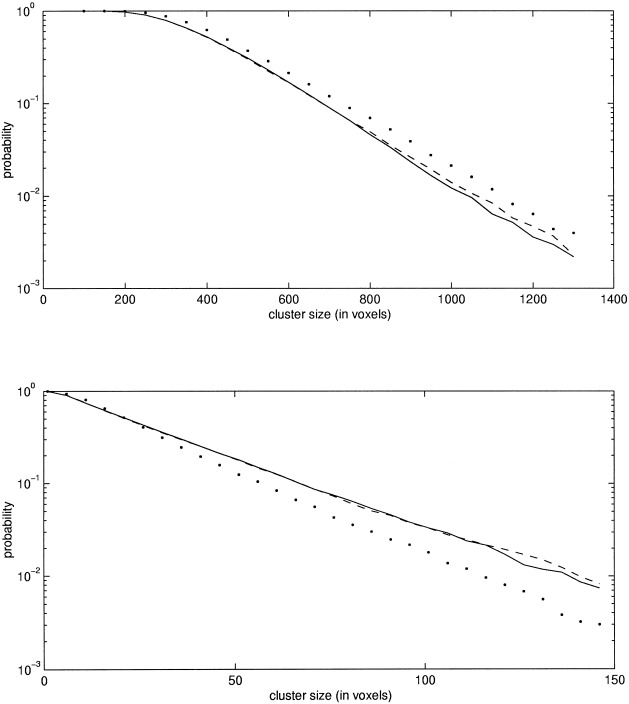
This figure shows the estimated probabilities of the cluster size statistic for the nonstationary dataset. In the upper figure, the threshold used was 2.0, and in the lower it was 3.457 and 3.454 for the MCS and randomization methods, respectively. The solid, dashed, and dotted lines refer to the MCS, randomization, and CS method, respectively.

Real PET Data

To evaluate the performance of the MCS method on real PET data, it was applied to the same dataset used in the evaluations in Ledberg et al. [1998]. A short description of the experiment and image preprocessing is given on the next page.

Six subjects participated in this study. They all gave informed consent. The study was approved by the local Ethics Committee and the Radiation Safety Committee of the Karolinska Hospital. Each subject was scanned in a PET scanner (SIEMENS‐CTI ECAT EXACT HR) during ten injections of 15‐O labeled butanol. The experimental paradigm consisted of two conditions each repeated five times. The conditions will be referred to as TEST and CONTROL. For each subject, the ten injections were divided into five blocks of two injections each. In each block, the order between TEST and CONTROL was randomized with the restriction that each block had to contain one TEST and one CONTROL condition. The TEST consisted in a two alternative forced choice tactile discrimination paradigm [Roland and Mortensen, 1987]. The subjects discriminated which of two aluminum parallellepipeda was the most oblong. They made the discrimination using active palpation with their right hand. In CONTROL, the subjects were lying in the PET scanner with their eyes closed and were instructed not to do or think anything in particular. Arterial radioactivity was continuously monitored during all injections. All data was acquired with the PET scanner operating in 3‐D mode. The images were reconstructed with a ramp filter having a cutoff frequency of 0.5 to a voxel size of 2 × 2 × 3.125 mm. In all images, only data in voxels contained inside the brain were used for further analysis, all other voxels were set to zero. This zeroing was done to prevent filtering in spurious data located outside the brain. The images were then filtered with a Gaussian filter of 6 mm FWHM in all dimensions. For each individual, the images from injections two to ten were aligned to the image from the first injection using the AIR‐software [Woods et al., 1992]. Regional cerebral blood flow (rCBF) was calculated using an autoradiographic method [Meyer, 1989]. Subsequently, we used information obtained from individual MR scans to reformat all images into a standard anatomical space [Roland et al., 1994] with cubic voxels of 2 × 2 × 2 mm. The global cerebral blood flow was normalized to 50 ml/100 gmin by multiplication by a constant.

The design matrix used to model the data is shown in Figure 1. The pd of the cluster size statistic for this model was estimated with the MCS and CS methods at two different thresholds corresponding to α = 0.01 and α = 0. 0005. The reference pd in this case was also generated using the randomization procedure. Unlike the above case of synthetic images, however, these real PET images do contain a strong signal that will make the distributions generated by the randomizations too conservative. However, by using the step‐down procedure described above, this bias can be minimized. For the present dataset, three steps were used and, at each step, the significant clusters at 0.05 level were removed. The number of randomizations was 5000 at each step. The pd obtained in the third step was used as the reference distribution. Because this pd is obtained from a subset of the original voxels (the voxels of the significant clusters in the previous two steps have been removed), the MCS and CS methods were also applied to the same subset of voxels. Thus, the pd derived from the CS and MCS methods and the reference pd were generated from the same set of voxels, and because these voxels do not contain any signal, the distributions should be the same. For the MCS and CS methods, 5000 simulations were used to estimate the pds. The results are shown in Figure 7. It is clear that, at both thresholds, the MCS method gives reliable estimates of the probabilities for probabilities higher than 0.01. Furthermore, it is clear from Figure 7 that the MCS method is better than the CS method because it gives an estimate closer to the one obtained by the randomizations.

Figure 7.

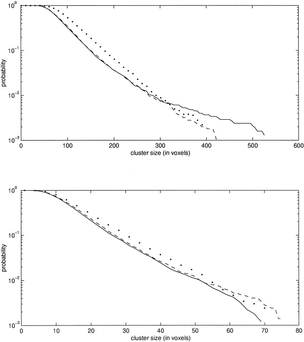
This figure shows the estimated probabilities of the cluster size statistic for the real PET dataset. The thresholds in the upper figure are 2.399, 2.400, and 2.33 for the randomization, MCS, and CS methods, respectively, and in the lower figure 3.484, 3.488, and 3.29. The dashed line corresponds to the reference distribution as determined with the randomization procedure (step three). The solid line shows the results of the MCS method and the dotted line shows the estimate obtained by the CS method. Please note that a logarithmic scale is used for the y‐axis.

DISCUSSION

MCS vs. CS

This paper has presented a novel way of estimating the probabilities of cluster sizes in PET images. The method is a modification of a previously presented method, the CS method of Ledberg et al. [1998]. Although very similar in spirit, there are some important differences between the two methods. In the CS method, it is assumed that the t‐images obtained under the null hypothesis are stationary and that they can be converted to a normal distribution (Gaussianized). These assumptions are not always valid. Furthermore, the relatively small sizes (i.e., number of voxels in each dimension) of the images makes the CS method less well suited for images with a broad autocorrelation function (acf) (i.e., smooth images). This is because the estimator of the acf [Eq. 2 in Ledberg et al., 1998] is noisy at large lags and smooth images will have a nonzero acf at large lags. Another drawback of the CS method (at least in its current implementation) is that it requires the user to set the value of a parameter used to scale the filter kernel used to generate the SSIs, so that the result can in this respect be dependent on the particular user. In the MCS method, on the other hand, the t‐images need not be stationary, they are not converted into a normal distribution, and there are no parameters to be set by the user. The only assumption needed in the MCS method is that the error terms in the model (Eq. 1) are distributed as N(0, I_n ⊗ Σ).

The validation showed that the MCS method gives accurate estimates of the pd of the cluster size statistic independent of the df of the models and the smoothness of the images. Furthermore, it was shown that the MCS method also gives good estimates on nonstationary images. This was in contrast to the CS method that did not work so well on these images (Fig. 6). That the CS method performed less well on the nonstationary images is not surprising because the estimator of the acf used assumes that the image is stationary. The impact of nonstationarity on the estimated pds will most likely vary depending on the source nonstationarity. Because it is unknown whether the SIs obtained in real PET experiments are stationary or not, one should perhaps be a little careful in using methods assuming stationarity. The comparison between the MCS and CS methods on the real PET data showed that the MCS method generated pds closer to the ones obtained by the randomizations. The CS method generated too conservative estimates, something that was observed also in Ledberg et al. [1998]. That the MCS method performed better on the real PET image might be because the assumption of stationarity is violated in these images. It could, however, have other explanations as well.

Because the MCS method gave better results than the CS method on both nonstationary and real PET data, it is indeed a significant improvement.

MCS vs. Randomizations

Because both the randomization and MCS methods require quite massive computations to estimate the pds for each dataset and, as shown in the validation, gives very similar estimates of the pds, it might seem that the MCS method is superfluous: why not always use the randomizations? However, the randomization approach has two drawbacks: (i) The number of possible randomizations can be very low for designs with a low df. This implies that the estimates might be conservative. (ii) Not all designs are suitable for randomization tests. Furthermore, if the images contain a signal, especially a strong signal, the estimated pds will be too conservative unless a (time‐consuming) step‐down approach is used. The MCS method does not suffer from these shortcomings. On the other hand, the MCS method relies on the assumption that the error terms in the linear model have a multivariate normal distribution. This assumption is not needed in the randomization approach. Another difference between the MCS and randomization methods is that the SSIs generated in the MCS method have df = λ − 1, whereas the original t‐images as well as the SSIs from the randomization have df = λ. However, this difference did not seem to matter if the appropriate thresholds were used, as shown in the validation.

Thus, the applicability of the MCS method complement that of the randomizations. The only limiting factor is the assumption of multivariate normality of the residuals. This assumption can probably be weakened to any distribution invariant under left multiplication by orthogonal matrices.

Random Field and Nonstationarity

To be able to apply the distributional results from random field theory, the SI need to be stationary. However, a technique developed recently by Keith Worsley and colleagues [Worsley et al., 1999] might be a way out of this limitation. Given a nonstationary SI, the idea is to warp this image into a new space where it is stationary. In this new space, one calculates the threshold corresponding to a desired α, applies this threshold, and then warps the image back to the original space.

Implementation

The MCS requires an estimation of the pd for each study where it is applied. These estimations are time consuming and require a computer with much memory. The current implementation required 512 Mbyte fast (100 MHz) RAM and the 5000 simulations on the real PET dataset took approximately 24 h on a computer with an Intel™ Pentium™ II processor of 400 MHz clock frequency. Probably, in studies with a very similar design and data preprocessing, the same cluster size thresholds will turn out to be significant. However, with small groups of subjects, some variance can be expected. The time to do one simulation is proportional to the square of the number of voxels times the number of scans (i.e., double the number of scans and the time it takes to make one simulation will increase by a factor of four). The software is available for Sun Solaris and Linux operative systems on request to the author.

CONCLUSIONS

The MCS method was shown to give accurate estimates of the probabilities of suprathreshold clusters in both stationary and nonstationary images. It was also shown to give “better” estimates than the CS method of Ledberg et al. [1998]. Thus, the MCS is a possible alternative to randomization tests in situations where the assumptions of the more theoretical approaches are violated.

Here, it is described how the simulated statistical images are generated both in the randomization and MCS methods. The assumption about the residuals in the randomization method is not really needed but it is used to show how closely related the two methods are. For proofs of some of the statements below, see Eaton [1983].

A Linear Model for the Data

Let Y be a n ×v matrix containing the observations, with n scans and v voxels per scan (v ≫n). Let

(A1)

be a linear model for the data in Y where X is the design matrix, B is a matrix containing the parameters, and E is a matrix of errors. The errors are assumed to be distributed as N(0, I_n ⊗ Σ). Let h be a testable contrast, then an estimate of hB is given by

(A2)

m _original is distributed as N(hB, h(X′X)⁻h′Σ) and an estimate of the variance of m _original is given by

(A3)

where M = (I − X(X′X(⁻ X′) and γ is the degrees of freedom of the model (i.e., n − rank(X)). By dividing the estimate of hB with the square root of the estimated variance, we get a t‐image:

(A4)

The two different approaches to generate simulated statistical images having a similar distribution to what t _original would have under the null hypothesis are described below.

Randomizations

Let P_i be a n ×n permutation matrix. Assume that the permutation described by P_i makes sense given the present design. Then let X_i = P_iX where X is the same design matrix as above. Then we have a new linear model for the data, namely, Y = X_iB_i+ E_i. Using the same contrast h as above we get

(A5)

and under the assumption that the residuals in the new model have the same distribution as the residuals in the old model, we have the following distribution of m _rand: N(hB_i, h(X′X)⁻ h′Σ). Thus, m _rand has the same variance–covariance structure as m _original. In complete analogy of how t _original was formed, we can now form t _rand. If the null hypothesis is true, the distribution of t _rand will be the same as that of t _original.

Simulations²

Let Y, X, M, and E be as above. Let R be the residuals of the model in Eq. (A1) (i.e., R = Y − XB = MY). R is distributed as N(0, M ⊗ Σ). Because M is an orthogonal projection, it can be decomposed into the product of two orthogonal matrices, M = KK′, say with K being of size n × γ. It then follows that K′R is distributed as N(0, I_γ ⊗ Σ) where I _γ is the identity matrix of size γ × γ. Let Γ_i be a random orthogonal matrix of size γ × γ. Because distributions of the type N(0, I_γ ⊗ Σ) are invariant under left multiplication by orthogonal matrices, it follows that Γ_iK′R is also distributed as N(0, I_γ ⊗ Σ). By dividing the mean of each column of Γ_iK′R with the estimated standard deviation of each column and multiplying with the square root of the degrees of freedom, we obtain t _simul. This image will have a distribution similar to what t _original would have had under the null hypothesis, but the df of this image is γ − 1, whereas the df in t _original is γ. However, by adjusting the threshold to yield the same α for the two different df, this should not matter. The orthogonal matrices Γ_i are generated by constructing an orthonormal basis for random normal matrices (distributed as N(0, I_γ ⊗ I_γ)) using a singular value decomposition [Press et al., 1992].

REFERENCES

- Cao J (1997): The excursion set of random fields with applications to human brain mapping. PhD thesis, Department of Mathematics and Statistics, McGill University, Montreal.
- Cao J (1999): The size of the connected components of excursion sets of χ2, t, and F fields. Adv Appl Prob. In press. [Google Scholar]
- Eaton M (1983): Multivariate statistic: A vector space approach. New York: Wiley. [Google Scholar]
- Edgington ES (1980): Randomization tests. New York: Dekker. [Google Scholar]
- Friston KJ, Frith CD, Liddle PF, Dolan RJ, Lammertsma AA, Frackowiak RSJ (1990): The relationship between global and local changes in PET scans. J Cereb Blood Flow Metab 10: 458–466. [DOI] [PubMed] [Google Scholar]
- Friston KJ, Frith CD, Liddle PF, Frackowiak RSJ (1991): Comparing functional (PET) images: The assessment of significant change. J Cereb Blood Flow Metab 11: 690–699. [DOI] [PubMed] [Google Scholar]
- Friston KJ, Worsley KJ, Frackowiak RSJ, Mazziotta JC, Evans AC (1994): Assessing the significance of focal activations using their spatial extent. Hum Brain Mapping 1: 210–220. [DOI] [PubMed] [Google Scholar]
- Graybill F (1976): Theory and application of the linear model. North Scituate: Duxbury Press. [Google Scholar]
- Holmes AP, Blair RC, Watson JDG, Ford I (1996): Nonparametric analysis of statistic images from functional mapping experiments. J Cereb Blood Flow Metab 16: 7–22. [DOI] [PubMed] [Google Scholar]
- Ledberg A, Åkerman S, Roland PE (1998): Estimating the significance of 3D clusters in functional brain images. NeuroImage 8: 113–128. [DOI] [PubMed] [Google Scholar]
- Meyer E (1989): Simultaneous correction for tracer arrival delay and dispersion in CBF measurements by the H215O autoradiographic method and dynamic PET. J Nucl Med 30: 1069–1078. [PubMed] [Google Scholar]
- Muirhead RJ (1982): Aspects of multivariate statistical theory. New York: Wiley. [Google Scholar]
- Press WH, Teukolsky SA, Vetterling WT, Flannery BP (1992): Numerical recipes in C (2nd Edition). Cambridge: Cambridge University Press. [Google Scholar]
- Roland PE, Mortensen E (1987): Somatosensory detection of microgeometry, macrogeometry and kinesthesia in man. Brain Res Rev 12: 1–42. [DOI] [PubMed] [Google Scholar]
- Roland PE, Graufelds CJ, Wåhlin J, Ingelman L, Andersson M, Ledberg A, Pedersen J, Åkerman S, Dabringhaus A, Zilles K (1994): Human brain atlas: For high‐resolution functional and anatomical mapping. Hum Brain Mapping 1: 173–184. [DOI] [PubMed] [Google Scholar]
- Woods RP, Cherry SR, Mazziotta JC (1992): Rapid automated algorithm for aligning and reslicing PET images. J Comput Assist Tomogr 16: 620–633. [DOI] [PubMed] [Google Scholar]
- Worsley KJ, Evans AC, Marrett S, Neelin P (1992): A three‐dimensional statistical analysis for CBF activation studies in human brain. J Cereb Blood Flow Metab 12: 900–918. [DOI] [PubMed] [Google Scholar]
- Worsley KJ, Marret S, Neelin P, Vandal AC, Friston KJ, Evans AC (1996): A unified statistical approach for determining significant signals in images of cerebral activation. Hum Brain Mapping 4: 58–73. [DOI] [PubMed] [Google Scholar]
- Worsley KJ, Andermann M, Koulis T, MacDonald D, Evans AC (1999): Detecting changes in nonstationary images via statistical flattening. NeuroImage 9: s11. [DOI] [PMC free article] [PubMed] [Google Scholar]