

Abstract
According to Friston, brain dynamics can be modelled as a large ensemble of coupled nonlinear dynamical subsystems with unstable and transient dynamics. In the present study, two predictions from this model (the existence of nonlinear synchronization between macroscopic field potentials and itinerant nonlinear dynamics) were investigated. The dependence of nonlinearity on the method of measuring brain activity (EEG vs. MEG) was also investigated. Dataset I consisted of 10 MEG recordings in 10 healthy subjects. Dataset II consisted of simultaneously recorded MEG (126 channels) and EEG (19 channels) in 5 healthy subjects. Nonlinear coupling was assessed with the synchronization likelihood S and dynamic itinerancy with the synchronization entropy Hs. Significance was assessed with a bootstrap procedure (“surrogate data testing”), comparing S and Hs with their distribution under the null hypothesis of stationary, linear dynamics. Significant nonlinear synchronization was detected in 14 of 15 subjects. The nonlinear dynamics were associated with a high index of itinerant behaviour. Nonlinear interdependence was significantly more apparent in MEG data than EEG. Synchronous oscillations in MEG and EEG recordings contain a significant nonlinear component that exhibits characteristics of unstable and itinerant behaviour. These findings are in line with Friston's proposal that the brain can be conceived as a large ensemble of coupled nonlinear dynamical subsystems with labile and unstable dynamics. The spatial scale and physical properties of MEG acquisition may increase the sensitivity of the data to underlying nonlinear structure. Hum. Brain Mapping 19:63–78, 2003. © 2003 Wiley‐Liss, Inc.
Keywords: MEG, EEG, synchronization, non‐linear, oscillations, dynamics, entropy
INTRODUCTION
Synchronization of activity within and between neuronal networks in the brain is currently the focus of intense research efforts [Bhattacharya 2001; Fries et al., 1997; Tallon‐Baudry et al., 2001; Varela et al., 2001]. This interest is due to the idea that synchronous oscillations may be an important mechanism by which specialized cortical and subcortical regions integrate their activity into a functional whole [Singer, 2001]. Thus, they are an important candidate solution for the so‐called “binding problem.” Synchronous oscillations in different frequency bands may correspond to different functions and different spatial scales of integration [Basar et al., 2001]. By and large, low frequencies in particular in the theta band, are hypothesized to play a role in coupling between distant brain regions (for instance prefrontal and post rolandic association cortices) whereas high frequencies are thought to be more important for short‐range interactions [von Stein and Sarnthein, 2000].
The importance of synchronous gamma band activity for object representation was first reported in animal studies in the early 1990s [Eckhorn et al., 1988; Engel et al., 1991; Gray et al., 1989]. This basic result has now been replicated many times, also in awake human subjects using EEG [Rodriguez et al., 1999; Tallon Baudry et al., 2001]. Synchronous gamma oscillations may provide a mechanism whereby complex objects are temporarily represented in working memory [Bertrand and Tallon‐Baudry, 2000] or a way to bind brain regions involved in associative learning into Hebbian cell assemblies [Miltner et al., 1999].
Local synchronization in the theta band has been associated with encoding and retrieval of information in episodic memory [Burgess and Gruzelier, 1997, 2000; Klimesch et al., 1994; Klimesch 1996, 1999]. Theta band coupling between frontal and post rolandic cortical regions has been reported during the retention interval of visual working memory tasks [Anokhin et al., 1999; Sarnthein et al., 1998; Stam, 2000] as well as during an N‐back working memory task [Ross and Segalowitz, 2000]. According to Anokhin et al. [ 1999] stronger theta band coherence is associated with a higher intelligence. Local desynchronization in the lower alpha band has been associated with attentional processes and upper alpha band desynchronization with semantic memory in a number of studies by Klimesch and coworkers [reviewed in Klimesch 1996, 1999]. The functional meaning of long distance coupling in the alpha band is less clear. Despite the fact that the importance of synchronous oscillations at different spatial scales and in different frequency bands for integrating brain activity is increasingly accepted, several questions need to be addressed. These questions relate to the origin and nature of synchronous oscillations and their relationship to optimal information processing in the brain. We discuss two ambitious models of brain dynamics that have attempted to deal with these issues.
In a series of studies, Edelman and co workers stressed that optimal information processing in the brain requires a delicate balance between local specialization and global integration/synchronization of brain activity [Tononi et al., 1994, 1998a,b]. They introduced a measure, the neural complexity or CN, which quantifies how optimal the balance between local specialization and global integration is [Tononi et al., 1994]. This measure was applied to fMRI data in Friston et al. [ 1995]. According to the model of Tononi et al., the neural complexity is expected to decrease during states of lower consciousness and impaired brain function. However, increased rather than decreased neural complexity has been reported during epileptic seizures and in Alzheimer's dementia, which is in disagreement with the predictions of the model [ Van Cappellen van Walsum et al., unpublished data; Van Putten and Stam, 2001].
A different concept of integrative brain dynamics has been put forward by Friston [ 2000a, 2000b, 2000c]. Friston models the brain as a large number of interacting nonlinear dynamical systems. The elementary states of such a system are designated “neural transients,” which can be thought of as brief spatiotemporal patterns of synchronous brain activity. Friston stresses the “labile” nature of normal brain dynamics, which consists of a rapid succession of neural transients and itinerant jumping between different marginally stable dynamical states (The terms “nonstationary,” “transient,” “unstable,” and “itinerant” may have different meanings in different contexts. To clarify the present use of these terms, we include a short list of definitions in the Appendix). In this model interactions between subsystems can be linear (as in the case of synchronous oscillations) as well as nonlinear. Nonlinear interactions between brain regions may reflect the unstable nature of brain dynamics including the changing modulatory influences of one frequency band on another (“asynchronous coupling”). In a modeling and experimental study, Breakspear [ 2002] demonstrated how interactions between coupled nonlinear dynamical systems can give rise to some of the phenomena described by Friston, and how such activity may contribute to the varying waveform of the alpha rhythm. In the model of Friston, optimal information processing is not obtained by a static balance between specialization and integration, but rather by unstable, nonlinear dynamics with rapidly fluctuating interactions [Friston, 2000b]. The model of Friston thus predicts that at least some of the interactions between brain regions will be nonlinear and transient. In contrast, the theory of Tononi et al. is compatible with linear and stationary dynamics.
There is some empirical evidence for (nonlinear) coupling between theta and gamma frequencies in EEG [Schack et al., 2001, 2002] and MEG recordings [Friston, 2000a]. Several studies have attempted to demonstrate nonlinear dynamics in normal EEG recordings. In most cases, nonlinearity was studied with measures that characterize local dynamics [Pritchard et al., 1995; Stam et al., 1999] or global dynamics [Rombouts et al., 1995]. The convergent finding of these studies is that nonlinear activity is present in scalp EEG data, at strong levels of significance, albeit only weakly and/or intermittently. Recent investigations of nonlinear interdependence between scalp EEG channels similarly report robust statistical evidence for nonlinear effects in approximately 5% of windowed epochs [Breakspear and Terry, 2002]. There is some evidence for nonlinear structure in MEG data [Kowalik et al., 2001] but nonlinear interactions between channels have not been studied.
To test the predictions of Friston a measure is needed that is sensitive to nonlinear interdependencies between time series and can deal with transient dynamics. Measures based upon the concept of generalized synchronization seem to be suited for this goal [Le van Quyen et al., 1998; Rulkov et al., 1995; Schiff et al., 1996]. In the pathological case of epileptic seizure activity nonlinear coupling between EEG signals has been demonstrated with this class of synchronization measures [Le van Quyen et al., 1998]. Recently, we introduced the synchronization likelihood, which is also based upon the concept of generalized synchronization but avoids some of the shortcomings of the other methods [Stam and van Dijk, 2002]. The synchronization likelihood characterizes linear as well as nonlinear synchronization between time series and can be computed with a high temporal resolution. From the synchronization likelihood a second measure, the synchronization entropy, can be computed. This measures the spatio‐temporal variability of synchronization, and thus reflects the presence of unstable dynamics. With the synchronization likelihood, a loss of functional connectivity in upper alpha, beta, and gamma frequency bands could be demonstrated in MEG recordings of Alzheimer patients [Stam et al., 2002b]. In healthy subjects, theta band synchronization likelihood as well as synchronization entropy were increased during the retention interval of a working memory task [Stam et al., 2002a].
The present study was undertaken to further explore the nature of synchronous activity in the brain and to test some of the predictions of the model proposed by Friston [ 2000a, 2000b, 2000c]. Three questions were addressed: (1) Is there evidence for nonlinear interactions between different neural networks in the brain? (2) If there is evidence for nonlinearity, to what extent is this related to transient or itinerant brain dynamics with rapidly fluctuating synchronization levels? (3) Are MEG recordings better able to detect nonlinear interactions than EEG recordings? To examine these questions, MEGs and EEGs recorded in 10 elderly and 5 young healthy subjects during a no‐task, eyes‐closed condition were studied with the synchronization likelihood and the synchronization entropy. The presence of nonlinear structure was tested statistically with phase randomised, multichannel surrogate data [Prichard and Theiler, 1994; Rombouts et al., 1995].
SUBJECTS AND METHODS
Subjects
In this study, recordings of two groups of healthy subjects were investigated. The first group (dataset I) consisted of ten healthy subjects (control subjects taken from a study on MEG changes in Alzheimer's disease). Mean age was 64.5 year (range: 53–74 years); three subjects were male. Three subjects were left‐handed (1 male). All subjects disavowed a history of cognitive dysfunction, and were screened for signs of cognitive decline/dementia. The protocol of this study was approved by the medical ethical Review Board of the Vrije Universiteit Medical Centre. All subjects or their relatives gave written informed consent after the nature of the procedure was explained. The second group (dataset II) consisted of five healthy subjects, all co‐workers of the MEG centre at the VU University medical centre (two females; mean age 30.5 year, range 25–38 years; all right‐handed).
MEG and EEG recordings
Magnetic fields were recorded while subjects were seated inside a magnetically shielded room (Vacuumschmelze GmbH, Germany) using a 151‐channel whole‐head MEG system (CTF Systems Inc., Canada). A third order software gradient (Vrba, 1996) was used with a recording passband of 0.25–125 Hz. Fields were measured during a no‐task, eyes‐closed condition. At the beginning and conclusion of each recording, the head position relative to the co‐ordinate system of the helmet was recorded by leading small AC currents through three head position coils attached to the left and right pre‐auricular points and the nasion on the subject's head. Head position changes during a recording condition up to approximately 1.5 cm were accepted.
In the case of dataset I, 16‐sec artefact‐free epochs (sample frequency 250 Hz; 4,096 samples) of MEG data were chosen for analysis. Of the original 151 channels, 34 were excluded either because their locations were too inferior for the registration of neural activity or because they contained significant artefacts in at least one of the subjects. This exclusion criteria permitted analysis of the same 117 channels in all subjects. The MEG data were band‐pass filtered off line between 0.5 and 40 Hz.
For dataset II, the MEG was recorded with the same system and the same settings as dataset I, except for a higher sample frequency of 625 Hz. These recordings were down‐sampled to 313 Hz and artefact‐free epochs of 13 sec (4,096 samples) were selected. In the case of dataset II, a larger number of channels (126) were artefact free in all subjects and, hence, were included in the analysis. For this dataset, EEG data were acquired simultaneously with the MEG. The EEG was recorded with Ag/AgCl electrodes from the following 19 positions of the international 10–20 system: Fp1, F7, F3, T7, C3, P7, P3, P1, Fz, Cz, Pz, Fp2, F8, F4, T8, C4, P8, P4, O2. The EEG was re‐referenced off line against an average reference electrode and digitally filtered between 0.5 and 40 Hz. The EEG epoch used for analysis coincided exactly with the MEG epoch. For both datasets, a subset of 19 MEG channels corresponding roughly with the location of the 19 EEG electrodes was also analysed.
Synchronization likelihood
The synchronization likelihood is a measure of the degree of synchronization or coupling between two or more time series [Stam and van Dijk, 2002]. An in‐depth description of the method and its performance with a variety of test and experimental signals can be found in the Stam and van Dijk study; here we give a more comprehensive description. The measure is based upon the concept of generalized synchronization as introduced by Rulkov et al. [ 1995]. Generalized synchronization is said to exist between two dynamical systems X and Y if there exists a continuous one‐to‐one function F such that the state of one of the systems (the response system) is mapped onto the state of the other system (the driver system): Y = F(X) [Abarbanel et al., 1996; Kocarev and Parlitz, 1996; Rulkov et al, 1995]. Intuitively, this means that generalized synchronization exists between two systems X and Y if the following holds: if X is in the same state at two different times i and j, Y will also be in the same state at times i and j. To make this concept operational, we need some concept of the state of a system, and a metric for the similarity of two states. This can be achieved by using the framework of nonlinear dynamical systems theory and state space embedding (a very accessible introduction can be found in Pritchard and Duke [ 1992]; a more recent but rather technical review is Schreiber [ 1999]).
We assume time series of measurements xi and yi (i = 1, …, N) recorded from X and Y. From these time series, we reconstruct vectors in the state space of X and Y (these vectors correspond to the “states” of both systems) with the method of time‐delay embedding [Takens, 1981]:
| (1) |
Here l is the time lag and m the embedding dimension. In a similar way vectors Yi are reconstructed from the time series yi. Now if the state of Y is a function of the state of X, each Xi will be associated with a unique Yi. Also if two vectors Xi and Xj are almost identical (the distance between Xi and Xj is very small) then, because of the continuity of F, Yi and Yj will also be almost identical. Thus, the distance between two vectors in state space is a metric of their similarity. We now have the required concepts of “state” and “similarity between states” and can continue to define a measure of synchronization in terms of these concepts.
The synchronization likelihood expresses the chance that if the distance between Xi and Xj is very small, the distance between Yi and Yj will also be very small. For this, we need a small critical distance ϵx, such that when the distance between Xi and Xj is smaller than ϵx, X will be considered to be in the same state at times i and j. ϵx is chosen such that the likelihood of two randomly chosen vectors from X (or Y) will be closer than ϵx (or ϵy) equals a small fixed number pref. It is important to note that pref is the same for X and Y, but ϵx need not be equal to ϵy. (Please note, that pref has nothing to do with a significance level; it is simply a way to control the value of S in the case no synchronization between the two systems exists.) Now the synchronization likelihood S between X and Y at time i is defined as follows:
| (2) |
Here we only sum over those j satisfying w1 <|i‐j|< w2, and Xi‐Xj< ϵx. N is number of j fulfilling these conditions. The value of w1 is the Theiler correction for autocorrelation and w2 is used to create a window (w1 < w2 < N) to sharpen the time resolution of Si (Theiler, 1986). When no synchronization exists between X and Y, Si will be equal to the likelihood that random vectors Yi and Yj are closer than ϵy; thus Si = pref. In the case of complete synchronization Si =1. Intermediate coupling is reflected by pref < Si < 1. Because pref is the same for X and Y, the synchronization likelihood is the same considering either X or Y as the driver system. Choosing pref the same for X and Y is necessary to ensure that the synchronization likelihood is not biased by the degrees of freedom or dimension of either X or Y [Stam and van Dijk, 2002].
From the basic definition of Si as given in equation (2), we can derive several variations by averaging over time, space or both. First, we can consider the average synchronization likelihood between X and two or more other systems. If we denote the index channel by k, Ski is the average synchronization between channel k and all other channel at time i. By averaging over all time points i we obtain Sk. Averaging over all channels k gives S, the overall level of synchronization in a multi channel epoch.
In the present study, the synchronization likelihood was computed with the following parameter settings: l = 10; m = 10; w1 = 100 (product of lag and embedding dimension); w2 = 400; pref = 0.05. The length of w1 and w2 is expressed in samples. There is no unique way to choose these parameters; however, the present parameter choices proved to be effective in distinguishing between experimental conditions in a working memory task [Stam et al., 2002a] and between MEG recordings of healthy controls and Alzheimer patients [Stam et al., 2002b].
Synchronization entropy
The strength of synchronization in an array of coupled nonlinear oscillators may be highly heterogeneous in both temporal and spatial domains, even if the coupling strength is constant. For example, in the setting of weakly coupled chaotic oscillators, the presence of intermittent bursts of desynchronization due to unstable periodic orbits has been the focus of much research [Heagy et al., 1998; Pecora, 1998; Pikovsky and Grassberger, 1991; Rulkov and Suschik, 1997]. This phenomenon results in an irregular pattern of phase synchrony over a wide range of temporal scales [Breakspear, 2002]. To characterize the variability of the synchronization likelihood Sk,i as a function of space as well as time we introduce the synchronization entropy Hs. The synchronization entropy is computed in a similar way as the Shannon information entropy. First the interval between pref and 1 is equipartitioned into N bins (in the present study, we used N = 100). Then we define pi as the likelihood that the value of Sk,i will fall in the ith bin. The entropy Hs is then obtained as,
| (3) |
When a logarithm with a base of 2 is used, the unit of Hs is bits. If there is no spatial and temporal variability in Sk,i then pi will equal 1 for one value of i, and 0 for all other i. In this case the entropy Hs will be zero. If there is maximal variability Sk,i can take all values in the interval between pref and 1 with equal probability and pi will equal 1/N for all i. The entropy Hs will then take its maximal value of log(N).
Multivariate surrogate data testing
The basic idea of surrogate data testing is to compute a nonlinear statistic Q from the original data, as well as from an ensemble of surrogate data [Theiler et al., 1992]. The surrogate data have the same linear properties (in particular power spectrum and coherence) as the original data, but are otherwise random. This permits testing of the null hypothesis H0 that the original data are linearly filtered Gaussian noise. This hypothesis is tested by computing a Z‐score:
| (4) |
The Z‐score expresses the number of standard deviations Q is away from the mean Qs of the surrogate data. Assuming that Q is approximately normally distributed in the surrogate data ensemble, the null hypothesis can be rejected at the P < 0.05 level when Z > 1.96. In the present study, we used two different nonlinear test statistics: the synchronization likelihood S (averaged over time and over all channels) and the synchronization entropy Hs. In both cases, an ensemble of 20 surrogate data was constructed from each original epoch.
The linear information in a time series is described completely by its power spectrum; in this case, the phases of the different frequencies are irrelevant. However, in the case of nonlinear structure within or between time series phase information is important. Thus, to test the null hypothesis that the original data only have linear information we need surrogate data that have exactly the same powerspectrum as the original data but random phases (thereby destroying any nonlinear information that may have been present). This type of surrogate data can be constructed by applying a Fourier transform to all MEG channels, adding a random number to the phase of each frequency, and then applying an inverse Fourier transform. For each frequency, the same random number was added to the phases of the different channels, thereby preserving exactly not only the power spectra of the individual channels but also the coherence between the channels [Prichard and Theiler, 1994; Rombouts et al., 1995].
RESULTS
The results of surrogate data testing using either the averaged synchronization likelihood S or the synchronization entropy Hs as a test statistic are shown in Table I for dataset I and in Table II for dataset II.
Table I.
Synchronization in Elderly Subjects
| Subject | No. ch. | S | S‐surr | S Z‐score | Hs | Hs‐surr | Hs Z‐score |
|---|---|---|---|---|---|---|---|
| C98‐10EC | 117 | 0.105 | 0.097 | 8.462 | 4.746 | 4.530 | 6.502 |
| 19 | 0.103 | 0.091 | 8.502 | 5.355 | 5.058 | 6.721 | |
| C98‐11EC | 117 | 0.093 | 0.088 | 5.566 | 4.551 | 4.401 | 4.589 |
| 19 | 0.084 | 0.078 | 6.188 | 4.916 | 4.724 | 4.471 | |
| C98‐12EC | 117 | 0.098 | 0.092 | 5.535 | 4.558 | 4.479 | 2.018 |
| 19 | 0.084 | 0.080 | 3.412 | 4.764 | 4.678 | 1.872 | |
| C98‐13EC | 117 | 0.108 | 0.102 | 4.559 | 4.752 | 4.706 | 1.121 |
| 19 | 0.093 | 0.087 | 4.078 | 4.801 | 4.745 | 1.148 | |
| C98‐14EC | 117 | 0.118 | 0.114 | 2.770 | 5.067 | 5.083 | −0.315 |
| 19 | 0.093 | 0.087 | 3.095 | 4.886 | 4.785 | 1.663 | |
| C98‐15EC | 117 | 0.104 | 0.098 | 5.242 | 4.705 | 4.612 | 2.230 |
| 19 | 0.085 | 0.079 | 4.815 | 4.717 | 4.567 | 3.242 | |
| C98‐16EC | 117 | 0.105 | 0.097 | 9.163 | 4.756 | 4.490 | 7.498 |
| 19 | 0.086 | 0.077 | 9.404 | 4.675 | 4.388 | 9.968 | |
| C99‐17EC | 117 | 0.110 | 0.101 | 7.506 | 4.941 | 4.711 | 5.054 |
| 19 | 0.093 | 0.088 | 3.104 | 4.882 | 4.829 | 1.024 | |
| C99‐18EC | 117 | 0.105 | 0.098 | 5.700 | 4.802 | 4.671 | 3.101 |
| 19 | 0.086 | 0.082 | 3.727 | 4.635 | 4.594 | 0.763 | |
| C99‐EC19 | 117 | 0.093 | 0.089 | 3.492 | 4.415 | 4.347 | 1.384 |
| 19 | 0.084 | 0.081 | 2.794 | 4.690 | 4.686 | 0.071 | |
| Mean | 117 | 0.104 | 0.098 | 6.190 | 4.729 | 4.616 | 3.908 |
| 19 | 0.090 | 0.080 | 4.912 | 4.832 | 4.705 | 3.764 |
Data set I. Synchronization likelihood (S) of original MEG data; mean synchronization likelihood of 20 surrogate data (S‐surr) and corresponding Z‐score (S Z‐score). Synchronization entropy of original MEG data (Hs); mean synchronization entropy of 20 surrogate data (Hs‐surr) and corresponding Z‐score (Hs Z‐score). The bottom row gives the mean values averaged over all 10 subjects. No. ch.: Number of MEG channels used in the analysis.
Table II.
Synchronization in Young Subjects
| Subject | Recording | S | S‐surr | S Z‐score | Hs | Hs‐surr | Hs Z‐score |
|---|---|---|---|---|---|---|---|
| AK‐OD | MEG126 | 0.106 | 0.097 | 7.586 | 5.046 | 4.815 | 4.724 |
| MEG19 | 0.094 | 0.085 | 4.162 | 5.112 | 4.947 | 3.043 | |
| EEG | 0.113 | 0.100 | 4.202 | 5.523 | 5.334 | 3.014 | |
| GdV‐OD | MEG126 | 0.105 | 0.099 | 4.857 | 4.900 | 4.821 | 1.377 |
| MEG19 | 0.088 | 0.080 | 6.195 | 4.860 | 4.761 | 2.230 | |
| EEG | 0.107 | 0.097 | 3.841 | 5.521 | 5.368 | 2.121 | |
| HM‐OD | MEG126 | 0.107 | 0.096 | 5.930 | 5.208 | 4.930 | 4.788 |
| MEG19 | 0.092 | 0.084 | 4.516 | 5.128 | 5.034 | 2.074 | |
| EEG | 0.198 | 0.184 | 2.230 | 6.537 | 6.448 | 1.212 | |
| JdM‐OD | MEG126 | 0.126 | 0.113 | 6.364 | 5.591 | 5.371 | 5.083 |
| MEG19 | 0.113 | 0.102 | 4.608 | 5.587 | 5.465 | 2.255 | |
| EEG | 0.213 | 0.183 | 4.272 | 6.426 | 6.405 | 0.305 | |
| JD‐OD | MEG126 | 0.092 | 0.091 | 1.222 | 4.879 | 4.784 | 1.505 |
| MEG19 | 0.079 | 0.078 | 0.317 | 4.877 | 4.811 | 1.339 | |
| EEG | 0.102 | 0.099 | 1.190 | 5.444 | 5.388 | 0.718 | |
| Mean | MEG126 | 0.107 | 0.099 | 5.192 | 5.125 | 4.944 | 3.495 |
| MEG19 | 0.093 | 0.086 | 3.960 | 5.113 | 5.004 | 2.188 | |
| EEG | 0.147 | 0.133 | 3.147 | 5.890 | 5.789 | 1.472 |
Data set II. Synchronization likelihood (S) of original MEG and EEG data; mean synchronization likelihood of 20 surrogate data (S‐surr) and corresponding Z‐score (S Z‐score). Synchronization entropy of original MEG data (Hs); mean synchronization entropy of 20 surrogate data (Hs‐surr) and corresponding Z‐score (Hs Z‐score). The bottom row gives the mean values averaged over all five subjects. MEG126 denotes the 126‐channel MEG analysis and MEG19 denotes the 19‐channel MEG analysis.
In all ten subjects of dataset I, the mean synchronization of the surrogate data was lower then the synchronization of the original data. The corresponding Z‐scores show that the null hypothesis could be rejected in all subjects, with Z‐scores ranging from 2.770 to 9.163 for the analysis with 117 channels and from 2.794 to 9.404 for the analysis with a subset of 19 channels. Consequently, there is strong statistical evidence in all subjects that the interdependence in the MEG data cannot be fully described by a stationary linear/stochastic model, and hence may contain nonlinear structure. Comparable results were obtained with the synchronization entropy Hs as test statistic: the mean entropy of the surrogate data was lower than the entropy of the original data in nine of the ten subjects for the analysis with 117 channels, and in all subjects for the analysis with 19 channels. The null hypothesis could be rejected in seven out of the ten subjects for the analysis with 117 channels and in four out of ten for the analysis with 19 channels.
Results of a more detailed analysis of a single representative subject (C98‐16EC) are shown in Figures 1 and 2. In both Figures 1 and 2, surrogate data testing was done using the Sk (average synchronization likelihood between channel k and all other channels) of all 117 channels as test statistics. Figure 1 shows Sk of the original MEG data (upper curve) and the distribution of Sk of each of the 20 surrogate data sets. It is clear that for most channels, Sk of the original data lies outside and above the range of Sk of the surrogate data. Note that this graphical comparison allows direct (non‐parametric) testing of the null hypothesis. The parametric test (based on estimation of the Z‐scores) is only necessary when adjusting for repeated comparisons. A one‐sample Kolmogorov Smirnov test on the distribution of S for the 20 surrogates showed that it did not differ significantly from the normal distribution (Kolmogorov‐Smirnov Z = 0.418; P = 0.995). Figure 2 shows the significance of the difference between Sk of the original data and Sk of the surrogate data, expressed as Z‐scores. For a significance level of P < 0.05, the null hypothesis could be rejected in 22 out of 117 channels, which is much higher than expected by chance (6 of 117).
Figure 1.

Dataset I. Results of surrogate data testing for a single subject (C98‐16EC). Sk (average synchronization likelihood between channel k and all other channels) was computed for all 117 channels of the original MEG data as well as for the 117 channels of the 20 surrogate data sets. The upper dotted curve with diamonds corresponds to the original data; the other 20 curves correspond to the distribution of the surrogate data. Sk of the original data is always higher than the Sk of any of the surrogate data.
Figure 2.

Same subject as in Figure 1. The curve shows the significance expressed as Z‐score of the difference between Sk of the original data and the mean Sk of the 20 surrogate data. For those channels where Z > 1.96, the null hypothesis can be rejected at the P < 0.05 level.
In the five subjects of dataset II, the mean synchronization of the surrogate data was also lower than the synchronization of the original data, although the difference was only marginal in the case of subject JD. This pattern was obvious for the 126‐channel and 19‐channel MEG data as well as for the EEG data. In each subject, the absolute synchronization likelihood was always higher in the EEG data than the MEG data, and higher for the 126‐channel than for the 19‐channel analysis. However, the opposite is true of the Z‐scores. In the case of the 126‐channel MEG data, the Z‐scores ranged from 1.22 to 7.59 (mean 5.19) and the null hypothesis could be rejected in four of the five subjects. For the 19‐channel MEG data, Z‐scores ranged from 0.317 to 6.195 and the null hypothesis could be rejected in the same four subjects as for the 126‐channel analysis. In the case of the EEG, Z‐scores ranged from 1.19 to 4.27 (mean 3.15), and the null hypothesis could be rejected in the same four subjects who showed significant results with MEG. In these four subjects, the Z‐scores for the 126‐channel MEG data were always much higher than the Z‐scores for the corresponding EEG data; for the 19‐channel MEG, this was the case in three of the four subjects (Fig. 3). The apparent contradiction (between the synchronization strengths and the Z‐scores) is a result of the synchronization measures for the surrogate data sets, which were on average much higher in the EEG data.
Figure 3.

Dataset II. Comparison of the significance of surrogate data testing for nonlinearity for simultaneous MEG (either 126 or 19 channels) and EEG recordings in each of five subjects. Test statistic was the synchronization likelihood. An ensemble of 20 surrogate data was used. For a Z‐score > 1.96, the null hypothesis can be rejected at the P < 0.05 level.
In all subjects of dataset II, the synchronization entropy was lower for surrogate data compared to original data, and for MEG (for 126 as well as 19 channel analysis) compared to EEG. For MEG Z‐scores ranged from 1.377 to 5.083 for the 126‐channel analysis, and from 1.339 to 3.043 for the 19‐channel analysis. The null hypothesis could be rejected in three out of five subjects at the 95% confidence level for the 126‐channel analysis and in four out of five subjects for the 19‐channel analysis. For EEG, the Z‐scores ranged from 0.718 to 3.014, and the null hypothesis could be rejected in two of the five subjects.
Mean results for MEG recordings in dataset I (bottom row of Table I) and dataset II (second to last row in Table II) were generally in good agreement. All MEG statistics were examined for statistical differences between the subjects of dataset I and dataset II with a t‐test (two‐sided; unequal variances). No significant differences were found at the P = 0.05 level with two minor exceptions: (1) Hs for the large number of channels was higher in dataset II (P = 0.035); (2) Hs‐surr for the large number of channels was also higher in dataset II (P = 0.032). However, after Bonferroni correction for multiple tests (adjusted P = 0.05/12 = 0.00417), these two differences are no longer significant. Thus, age differences between the subjects of dataset I and II do not affect the experimental measures.
For the subjects in dataset I, the Z‐scores for the 117‐ and the 19‐channel analysis were strongly correlated, although the 19‐channel Z‐scores were slightly lower. This is illustrated in Figure 4.
Figure 4.
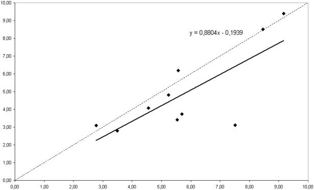
Dataset I. Correlation for each of the 10 subjects of the Z‐score obtained with 117 MEG channels (on the x‐axis) and the Z‐score obtained with the sub‐selection of 19 channels (on the y‐axis). The line indicates the a linear fit of the data; the corresponding model is shown (top right).
DISCUSSION
The present study was performed to answer the following three questions: (1) Is there evidence for significant nonlinear synchronization between brain regions in healthy subjects during a no‐task eyes‐closed state? (2) Does this nonlinearity have a stable or an unstable, itinerant character? (3) Are MEG recordings more suitable to detect nonlinear synchronization than EEG recordings? We will consider the results of the present study in relation to these three questions.
The results obtained with both data sets strongly suggest the presence of nonlinear synchronization in multichannel MEG data sets. Using the averaged synchronization S as a test statistic, the null hypothesis that all couplings can be described with a linear model could be rejected in all ten subjects of dataset I, and in four of five subjects in data set II. The level of significance was usually very high, with Z‐scores > 4 (corresponding with P < 0.00005) in 12 of 15 subjects. We interpret these results as supporting the presence of nonlinear coupling across multiple cortical regions in healthy human subjects. However, to assess the validity of these results, three issues deserve mentioning: (1) the use of a parametric statistical test to reject the null hypothesis; (2) the possibility of type I statistical errors; (3) the reliability of phase‐randomized surrogate data.
First, we compared the S of the original MEG data with the mean S obtained from an ensemble of 20 surrogate data (S‐surr) for each subject by computing a Z‐score; the Z‐score quantifies the distance between S and S‐surr in terms of the standard deviations of S‐surr. The tacit assumption is that S‐surr is approximately normally distributed, which may not be true. In theory, it is possible that a non‐Gaussian distribution of S in the surrogate data ensemble will bias the test of the null hypothesis. To avoid this bias, the null hypothesis can also be tested in a non‐parametric manner [Rapp et al., 1994]. When S of the original data is larger then S of each of the 20 surrogate data, then for a one‐sided test the null hypothesis can be rejected at the P < 0.05 level. In Figure 1, we show that this is the case for one representative subject: Sk of the original data is always higher then Sk of the surrogate data. In conclusion, we think it is unlikely that our results are due to a non‐Gaussian distribution of S in the surrogate data sets. Also, assessment of very high significances with non‐parametric tests is problematic because it would require ensembles of hundreds to thousands of surrogate data for each subject, which is computationally prohibitive. To test the null hypothesis two‐sided at a level of P = psignificance with a non‐parametric test, we need to generate an ensemble of N surrogate data where N can be determined as follows: psignificance = 1/(N‐2).
Second, to test the null hypothesis we used an alpha level of P < 0.05 in each individual subject. Because 15 subjects were investigated, there is a chance of type I statistical error (spurious rejections of the null hypothesis due to multiple independent tests). However, if we apply a rigorous Bonferroni correction, and use an adjusted significance level of P < 0.05/15 or P < 0.0033 (Z > 2.12), the conclusions remain the same and we can still reject the null hypothesis in 14 of 15 subjects.
Finally, the reliability of the procedure to generate surrogate data needs to be considered. Ideally, surrogate data preserve only but exactly the linear properties (power spectrum; coherence) of the original data. Any differences between original and surrogate data can then be ascribed to nonlinear properties of the original data. Problems can arise in two circumstances: (1) When the amplitude distribution of the original data is non‐Gaussian; (2) When the basic frequencies of the original data do not match exactly with the frequencies of the discrete Fourier transform. The latter problem typically arises with (nearly) periodic time series In the case of univariate time series, these problems are well known, and procedures to avoid them have been proposed [Stam et al., 1998; Theiler et al., 1992]. Whether the same problems also affect surrogate data testing for nonlinear couplings between time series in multivariate data sets is unknown. To address this problem, we considered a simple model system, consisting of two identical time series (4,096 samples). Each time series was the absolute value of a sine wave; the period of the sine wave was chosen such that it did not match with the length of the time series. Thus, the time series have the two features (non‐Gaussian amplitude distribution and non‐matching frequency) that are known to bias within channel surrogate data testing; however, because both time series were identical, the coupling between the channels was linear. Surrogate data testing of this test system (using synchronization likelihood as a test statistic and 20 surrogate data sets) did not produce spurious rejections of the null hypothesis. This suggests that testing for nonlinear coupling in multivariate data sets with the synchronization likelihood is not affected by non‐Gaussian amplitude distribution and frequency mismatch. However, further systematic study of this is warranted.
The nonlinear nature of the couplings between brain regions may be associated with several interesting phenomena. Friston [ 2000a] considers two aspects of nonlinear coupling: (1) Interactions between different frequencies, in particular theta and gamma band, and (2) Labile and unstable dynamics arising from a rapid succession of “neural transients.” There is some empirical evidence for (nonlinear) coupling between theta and gamma frequencies in EEG [Schack et al., 2001, 2002], microelectrode [Schanze and Eckhorn, 1997], and MEG recordings [Friston, 2000a] and across a broad range of frequencies in multichannel EEG data [Breakspear and Terry, 2002]. In the present study, we focused on the labile and unstable aspect of nonlinearity. The synchronization entropy Hs is a measure that characterizes the spatial and temporal variability of the synchronization likelihood Ski. With one exception, Hs of the original MEG data was always higher than Hs of the surrogate data set. If we use Hs as a test statistic, the null hypothesis can be rejected in 10 of 15 subjects (or 9 of 15 with Bonferroni correction). The Z‐scores for S were always higher than the Z‐scores for Hs. From these results, two conclusions can be derived. First, the original MEG data are considerably more variable than the surrogate data. So at least part of the nonlinear nature of coupling in MEG data may be associated with either transient or itinerant nonlinear dynamics. Second, Hs discriminated less well between original and surrogate data then S. This suggests that the nonlinearity in the original MEG data is not completely explained by unstable dynamics. Different factors, such as stable coupling between different frequency bands, probably play a role and need to be addressed in further studies.
In dataset II, a comparison was made between nonlinearity in MEG and EEG data sets. As can be seen in Table II and Figure 3, using S as a test statistic Z‐scores were usually higher for MEG than for EEG, sometimes considerably so. However, both with MEG and EEG the null hypothesis could be rejected in four of five subjects. In the case of Hs, the MEG Z‐score was also higher than the EEG Z‐score in four of five subjects. Thus, while nonlinear synchronization may be more easily detected in MEG then in EEG, MEG and EEG results are quite consistent. The greater sensitivity of MEG could be due to several factors. (1) MEG channels are sensitive to electrical current fluctuations on a smaller spatial scale than scalp EEG electrodes. Nonlinear waves are characterized by highly coherent phase characteristics. However, such structure may be lost at the spatial scale of EEG data due to summation of multiple uncorrelated waves arising through volume conduction. This linear summation of uncorrelated nonlinear waves is supported by the finding of increased overall synchronization likelihood in EEG data (and their surrogates) but decreased Z‐scores for the nonlinear contribution. In other words, volume conduction leads to greater linear “flooding” of underlying nonlinear synchronization. (2) MEG data is recorded without a reference. The reference that has to be used in the case of EEG influences the assessment of couplings between EEG channels [Nunez et al., 1997]. The influence of reference on nonlinear EEG measures was already demonstrated by Dvorak [ 1990]. (3) Finally, detection of nonlinearity with MEG may have been favoured by the larger number of MEG channels (117 in dataset I and 126 in dataset II) as compared to the number of EEG channels (19). Using such large numbers of channels is more practical with more whole head MEG systems, and it makes more sense also because of the higher spatial resolution of MEG compared to EEG. However, the results for either the full number of MEG channels or 19‐channel selections show that the extra information obtained in this way is quite modest. Further investigation, involving large subject numbers and a variety of MEG channel selections, is required in order to verify that MEG data is more sensitive to underlying nonlinear structure than EEG, and to establish which of the above mechanisms are the principle causes.
So far, most studies have investigated nonlinearity of brain dynamics using EEG [Pritchard et al., 1995; Rombouts et al., 1995; Stam et al., 1999] rather then MEG [Kowalik et al., 2001]. Usually, nonlinearity was assessed within rather than between channels [Pritchard et al., 1995; Stam et al., 1999]. As indicated above, surrogate data testing applied to univariate time series can be biased by several problems [Stam et al., 1998; Theiler et al., 1992]. When these problems are dealt with, nonlinearity can only be detected in a minority of subjects [Stam et al., 1999].
Rombouts et al. [ 1995] used the correlation dimension computed from a spatial embedding as a test statistic (mixing within and between channel information) and found evidence for nonlinear dynamics in 7 out of 15 healthy subjects. Comparing the results of the present study with the older EEG literature, we may conclude that nonlinear structure in brain dynamics is more easily detected with MEG then with EEG and that it may be more effective to focus upon nonlinear synchronization between channels rather than to look for nonlinear structure within channels.
The main results of the present study are in agreement with the model proposed by Friston [ 2000a, 2000b, 2000c]. Two important predictions derived from this model, the presence of nonlinear synchronization between brain regions and the unstable, or “labile” character of brain dynamics, were confirmed. This supports an approach to brain modelling based upon study of coupled nonlinear dynamical subsystems [e.g., Frank et al., 2000]. Such systems display dynamical phenomena that are not only in agreement with empirical observations but that also suggest mechanisms of information processing, such as the representation of external stimuli by dynamical attractors in neural systems, permitting their unique perception [Breakspear, 2001]. When two nonlinear dynamical systems are coupled, they may display different types of behaviour depending upon the strength of the coupling [Breakspear, 2002]. In the case of very weak, but also, paradoxically, in the case of very strong nonlinear coupling, the systems may show a low level of synchronization. However, for intermediate coupling, intermittent behaviour may emerge. This consists of brief episodes of strong synchronization, intermixed with episodes of desynchronised dynamics. This kind of critical dynamics provides a mechanism whereby synchronous cell assemblies can be established as well as rapidly deconstructed. Optimal information processing could depend upon an optimal balance between synchronization and desynchronization, which is obtained by such itinerant nonlinear dynamics. The concept of brief, unstable episodes of synchronous oscillations (the “neural transients” of Friston) intermixed by desynchronization has also been suggested by the modelling work of other authors [Freeman and Rogers, 2002; Hopfield and Brody, 2001]. Hopfield and Brody suggest that “The fundamental recognition event [in a neural network] is a transient collective synchronization” and also that “If such synchronization is used in neurobiological computation, its hallmark will be a brief burst of gamma‐band electroencephalogram noise when and where such a recognition or decision occurs.” In line with this, Freeman and Rogers [ 2002] speak of “Phase locking for brief time segments punctuated by episodic phase decoherence.” The results of the present study provide empirical support for the existence of such transient dynamical events because the synchronization entropy of the original MEG data is much higher then that of the surrogate data. When the synchronization likelihood is computed as a function of space as well as time (Ski) for MEG data filtered in the gamma band, episodes of synchronization can be seen lasting 100 to 500 msec, intermixed with desynchronization [fig. 10 in Stam and van Dijk, 2002]. Further studies on the nature of functional interactions in the brain will have to take into account the existence of nonlinear synchronization between brain regions, unstable phenomena in the form of brief neural transients, interactions across different frequency bands, and ongoing cognitive activity.
Acknowledgements
We thank Alexandra Linger for help preparing the manuscript, and Wim de Rijke as well as Jeroen Verbunt for technical support. The two anonymous referees are thanked for their helpful comments and suggestions.
DEFINITION OF TERMS
In the literature, one often finds terms relating to changing activity in a system, such as “nonstationary,” “transient,” or “unstable” used differently in different contexts. For the sake of clarity in the present work, we offer the following definitions of terms, and examples of models in which they may occur.
Stationary stochastic time series
“Stationarity” is typically used in the context of stochastic linear models. In this context, it refers to time series that have non‐varying probability measures, such as mean, variance, or spectrum. Such time series can be described by autoregressive stochastic models of the form,
| (A1) |
where the Ai and B are the fixed probability parameters and y is a white noise signal.
Nonstationary stochastic time series
“Nonstationarity” is also typically used in the context of linear/stochastic modelling. It refers to time series that have time‐dependent probability measures, such as changing spectral properties. Autoregressive moving average models (ARMA) may be used to describe such time series. These are of a similar form as (A1), except the coefficients are time‐dependent,
| (A2) |
All‐night sleep EEG may be viewed as nonstationary.
Nonlinear deterministic processes
The modern theory of nonlinear dynamical systems typically refers to the study of nonlinear differential or difference equations, and this is how the term is employed in the present study. These are of the form,
| (A3) |
| (A4) |
where a is a real‐valued vector that smoothly parameterises F. One seeks solution curves, or orbits, to such equations in the system's multi‐dimensional phase space, originating from various initial states, x(0). Attractors are sets that contain long‐term (asymptotic) solutions of the orbits of a “large number” of initial states [Milnor, 1985]. Attractors may be steady state, periodic, quasiperiodic, or chaotic. This simple formulation allows us to distinguish between a number of types of different time‐varying dynamical states.
Transient nonlinear dynamics
Traditionally, the term “chaotic transience” was applied in the following way [Greborgi et al., 1983]: A chaotic attractor, subject to some parameter perturbation, “collides” with its own basin boundary. Consequently, orbits on the attractor are mapped into another basin and, subsequently, onto another attractor. Put another way, the former attractor is no longer an invariant of the dynamic. However, a large set of initial conditions will transiently “shadow” the former attractor (now an attractor “ruin”), hence briefly mimicking its behaviour, before collapsing onto an alternative attractor.
Itinerant nonlinear dynamics
It has often been observed that a low‐dimensional manifold (of much lower dimension than the entire phase space) will contain a set that, whilst not an attractor, attracts the dynamics for significant periods of time [e.g.. Ashwin, 1995; Platt et al. 1993]. Between such times, the system may intermittently burst from this more ordered state into high‐dimensional dynamics. Such a process creates a complex time series because the bursting behaviour may follow a log‐log scaling law [e.g., Yu et al., 1991]. This process is particularly important in the context of sparsely coupled nonlinear subsystems, such as the brain, where the low‐dimensional activity corresponds to synchronization and the intermittent bursting to high‐dimensional desynchronization [e.g., Breakspear, 2002; Heagy et al., 1998; Yang and Ding, 1996]. Friston [ 2000b] refers to this as “type II complexity.” In the present study, due to the focus on nonlinear synchronization and its variation on small temporal scales, we favour this interpretation of nonlinear instability. Itinerancy is unlike transience in that it does not abate after a period of time.
Nonstationary nonlinear dynamics
In the setting of nonlinear itineracy, the dynamics are highly unstable due the structure of the flow in the phase space, but the orbits (or more correctly, the vector fields) are themselves unchanging. In contrast, it is possible to produce fluctuating dynamical states by making the state parameters themselves time‐dependent. In this way, the vector field, and hence the direction of the orbits, are themselves changing. Attractors are continually being formed, then “ruined” and possibly remade according to the nature of the state parameters. In such a case, one expects a type of “continuous transience” as the system moves between towards and then away from regions of phase space where attractors are ruined and rebuilt [Breakspear and Friston 2001; Friston, 1997; Tsuda, 2001]. Friston [ 2000b] refers to these dynamics as “type I complexity.”
REFERENCES
- Abarbanel H, Rulkov N, Sushchik M. (1996): Generalised synchronisation of chaos: The auxillary system approach. Phys Rev E 53: 4528–4535. [DOI] [PubMed] [Google Scholar]
- Anokhin AP, Lutzenberger W, Birbaumer N. (1999): Spatiotemporal organization of brain dynamics and intelligence: an EEG study in adolescents. Int J Psychophysiol 33: 259–273. [DOI] [PubMed] [Google Scholar]
- Ashwin P. (1995): Attractors stuck on to invariant subspaces. Phys Lett A 209: 338–344. [Google Scholar]
- Basar E, Basar‐Eroglu C, Karakas S, Schurmann M. (2001): Gamma, alpha, delta, and theta oscillations govern cognitive processes. Int J Psychophysiol 39: 241–248. [DOI] [PubMed] [Google Scholar]
- Bertrand O, Tallon‐Baudry C. (2000): Oscillatory gamma activity in humans: a possible role for object representation. Int J Psychophysiol 38: 211–223. [DOI] [PubMed] [Google Scholar]
- Bhattacharya J, Petsche H, Feldman U, Rescher B. (2001): EEG gamma‐band phase synchronization between posterior and frontal cortex during mental rotation in humans. Neurosci Lett 311: 29–32. [DOI] [PubMed] [Google Scholar]
- Breakspear M. (2001): Perception of odors by a nonlinear model of the olfactory bulb. Int J Neural Syst 11: 101–124. [DOI] [PubMed] [Google Scholar]
- Breakspear M, Friston K. (2001): Symmetries and itinerancy in nonlinear systems with many degrees of freedom. Behav Brain Sci 24: 813–814. [Google Scholar]
- Breakspear M. (2002): Nonlinear phase desynchronization in human electroencephalographic data. Hum Brain Mapp 15: 175–198. [DOI] [PMC free article] [PubMed] [Google Scholar]
- Breakspear M, Terry J. (2002): Detection and description of nonlinear interdependence in normal multichannel human EEG. Clin Neurophysiol 113: 735–753. [DOI] [PubMed] [Google Scholar]
- Burgess AP, Gruzelier JH. (1997): Short duration synchronization of human theta rhythm during recognition memory. Neuroreport 8: 11039–1042. [DOI] [PubMed] [Google Scholar]
- Burgess AP, Gruzelier JH. (2000): Short duration power changes in the EEG during recognition memory for words and faces. Psychophysiology 37: 596–606. [PubMed] [Google Scholar]
- Dvorak I. (1990): Takens versus multichannel reconstruction in EEG correlation exponent estimates. Phys Lett A 151: 225–233. [Google Scholar]
- Eckhorn R, Bauer R, Jordan W, Brosch M, Kruse W, Munk M, Reitboeck HJ. (1988): Coherent oscillations: a mechanism of feature linking in the visual cortex? Multiple electrode and correlation analyses in the cat. Biol Cybern 60: 121–130. [DOI] [PubMed] [Google Scholar]
- Engel AK, Kreiter AK, Konig P, Singer W. (1991): Synchronization of oscillatory neuronal responses between striate and extrastriate visual cortical areas of the cat. Proc Natl Acad Sci U S A 1991; 88: 6048–6052. [DOI] [PMC free article] [PubMed] [Google Scholar]
- Frank T, Daffertshofer A, Peper C, Beek P, Haken H. (2000): Toward a comprehensive theory of brain activity: coupled oscillators under external forces. Physica D 144: 62–86. [Google Scholar]
- Freeman WJ, Rogers LJ. (2002): Fine temporal resolution of analytic phase reveals episodic synchronization by state transitions in gamma EEGs. J Neurophysiol 2002; 87: 937–945. [DOI] [PubMed] [Google Scholar]
- Fries P, Roelfsema PR, Engel AK, Konig P, Singer W. (1997): Synchronization of oscillatory responses in visual cortex correlates with perception in interocular rivalry. Proc Natl Acad Sci U S A 94: 12699–12704. [DOI] [PMC free article] [PubMed] [Google Scholar]
- Friston KJ. (1997): Another neural code? Neuroimage 5: 213–220. [DOI] [PubMed] [Google Scholar]
- Friston KJ. (2000a): The labile brain. I. Neuronal transients and nonlinear coupling. Phil Trans R Soc Lond B 355: 215–236. [DOI] [PMC free article] [PubMed] [Google Scholar]
- Friston KJ. (2000b): The labile brain. II. Transients, conplexity and selection. Phil Trans R Soc Lond B 355: 237–252. [DOI] [PMC free article] [PubMed] [Google Scholar]
- Friston KJ. (2000c): The labile brain. III. Transients and spatio‐temporal receptive fields. Phil Trans R Soc Lond B 355: 253–265. [DOI] [PMC free article] [PubMed] [Google Scholar]
- Friston KJ, Tononi G, Sporns O, Edelman G. (1995): Characterising the complexity of neuronal interactions. Hum Brain Mapp 1995; 3: 302–314. [Google Scholar]
- Gray CM, Konig P, Engel AK, Singer W. Oscillatory responses in cat visual cortex exhibit inter‐columnar synchronization which reflects global stimulus properties. Nature 1989; 338: 334–337. [DOI] [PubMed] [Google Scholar]
- Greborgi C, Ott E, Yorke J. (1983): Crises, sudden changes in chaotic attractors and chaotic transients Physica D 7: 181–200. [Google Scholar]
- Heagy J, Carroll T, Pecora L. (1998): Desynchronization by periodic orbits. Phys Rev E 52: R1253–R1256. [DOI] [PubMed] [Google Scholar]
- Hopfield JJ, Brody CD. (2001): What is a moment? Transient synchrony as a collective mechanism for spatiotemporal integration. Proc Natl Acad Sci U S A 98: 1282–1287. [DOI] [PMC free article] [PubMed] [Google Scholar]
- Klimesch W. (1996): Memory processes, brain oscillations and EEG synchronization. Int J Psychophysiol 24: 61–100. [DOI] [PubMed] [Google Scholar]
- Klimesch W. (1999): EEG alpha and theta oscillations reflect cognitive and memory performance: a review and analysis. Brain Res Rev 29: 169–195. [DOI] [PubMed] [Google Scholar]
- Klimesch W, Schimke H, Schwaiger J. (1994): Episodic and semantic memory: an analysis in the EEG theta and alpha band. Electroenceph Clin Neurophysiol 91: 428–441. [DOI] [PubMed] [Google Scholar]
- Kocarev, L ., Parlitz, U . (1996): Generalised synchronisation, predictability and equivalence of unidirectionally coupled dynamical systems. Phys Rev Lett 76: 1816–1819. [DOI] [PubMed] [Google Scholar]
- Kowalik ZJ, Schnitzler A, Freund H‐J, Witte OW. (2001): Local Lyapunov exponents detect epileptic zones in spike‐less interictal MEG recordings. Clin Neurophysiol 112: 60–67. [DOI] [PubMed] [Google Scholar]
- Milnor J. (1985): On the concept of attractor. Commun Math Phys 99: 177–195. [Google Scholar]
- Miltner WHR, Braun C, Arnold M, Witte M, Taub E. (1999): Coherence of gamma‐band EEG activity as a basis for associative learning. Nature 397: 434–436. [DOI] [PubMed] [Google Scholar]
- Nunez PL, Srinivasan R, Westdorp AF, Wijesinghe RS, Tucker DM, Silberstein RB, Cadusch PJ. (1997): EEG coherency I: statistics, reference electrode, volume conduction, Laplacians, cortical imaging, and interpretation at multiple scales. Electroenceph Clin Neurophysiol 103: 499–515. [DOI] [PubMed] [Google Scholar]
- Pecora L. (1998): Synchronization conditions and desynchronizing patterns in coupled limit‐cycle and chaotic systems. Phys Rev E 58: 347–360. [Google Scholar]
- Pikovsky A, Grassberger P. (1991): Symmetry breaking bifurcation for coupled chaotic attractors, J Phys A 24: 4587–4597. [Google Scholar]
- Platt N, Spiegel E, Tresser C. (1993): On‐off intermittency: A mechanism for bursting. Phys Rev Lett 70: 279–282. [DOI] [PubMed] [Google Scholar]
- Prichard D, Theiler J. (1994): Generating surrogate data for time series with several simultaneously measured variables. Phys Rev Lett 73: 951–954. [DOI] [PubMed] [Google Scholar]
- Pritchard WS, Duke DW. (1992): Measuring chaos in the brain: a tutorial review of nonlinear dynamical EEG analysis. Int J Neurosci 67: 31–80. [DOI] [PubMed] [Google Scholar]
- Pritchard WS, Duke DW, Krieble KK. (1995): Dimensional analysis of resting human EEG II: Surrogate data testing indicates nonlinearity but not low‐dimensional chaos. Psychophysiology 32: 486–491. [DOI] [PubMed] [Google Scholar]
- van Putten MJAM, Stam CJ. (2001): Application of a neural complexity measure to multichannel EEG. Phys Lett A 281: 131–141. [Google Scholar]
- Quyen M Le Van, Adam C, Baulac M, Martinerie J, Varela FJ. (1998): Nonlinear interdependencies of EEG signals in human intracranially recorded temporal lobe seizures. Brain Res 792: 24–40. [DOI] [PubMed] [Google Scholar]
- Rodriguez E, George N, Lachauz JP, Martinerie J, Renault B, Varela FJ. (1999): Perception's shadow: long distance synchronization of human brain activity. Nature 397: 430–433. [DOI] [PubMed] [Google Scholar]
- Rapp PE, Albano AM, Zimmerman ID, Jimenez‐Montano MA. (1994): Phase‐randomized surrogates can produce spurious identifications of non‐random structure. Phys Lett A 192: 27–33. [Google Scholar]
- Rombouts SARB, Keunen RWM, Stam CJ. (1995): Investigation of nonlinear structure in multichannel EEG. Phys Lett A 202: 352–358. [Google Scholar]
- Ross P, Segalowitz SJ. (2000): An EEG coherence test of the frontal versus dorsal ventral hypothesis in N‐back working memory. Brain Cognit 43: 375–379. [PubMed] [Google Scholar]
- Rulkov N, Sushchik M, (1997): Robustness of synchronized chaotic oscillations. Int J Bifurc Chaos 7: 625–643. [Google Scholar]
- Rulkov NF, Sushchik MM, Ysimring LS, Abarbanel HDI. (1995): Generalized synchronization of chaos in directionally coupled chaotic systems. Phys Rev E 51: 980–994. [DOI] [PubMed] [Google Scholar]
- Sarnthein J, Petsche H, Rappelsberger P, Shaw GL, von Stein A. (1998): Synchronization between prefrontal and posterior association cortex during human working memory. Proc Natl Acad Sci U S A 95: 7092–7096. [DOI] [PMC free article] [PubMed] [Google Scholar]
- Schack B, Rappelsberger P, Vath N, Weiss S, Moller E, Griessbach G, Witte H. (2001): EEG frequency and phase coupling during human information processing. Methods Inform Med 40: 106–111. [PubMed] [Google Scholar]
- Schack B, Vath N, Petsche H, Geissler H‐G, Moller E. (2002): Phase‐coupling of theta‐gamma EEG rhythms during short‐term memory processing. Int J Psychophysiol 44: 143–163. [DOI] [PubMed] [Google Scholar]
- Schanze T, Eckhorn R (1997): Phase correlation among rhythms present at different frequencies: spectral methods, application to microelectrode recordings from visual cortex and functional implications. Int J Psychophysiol 26: 171–189. [DOI] [PubMed] [Google Scholar]
- Schiff SJ, So P, Chang T. (1996): Detecting dynamical interdependence and generalized synchrony through mutual prediction in a neural ensemble. Phys Rev E 54: 6708–6724. [DOI] [PubMed] [Google Scholar]
- Schreiber Th. Interdisciplinary application of nonlinear time series methods. Phys Rep 1999; 308: 1–64. [Google Scholar]
- Singer W. (2001): Consciousness and the binding problem. Ann NY Acad Sci 929: 123–146. [DOI] [PubMed] [Google Scholar]
- Stam CJ. (2000): Brain dynamics in theta and alpha frequency bands and working memory performance in humans. Neurosci Lett 286: 115–118. [DOI] [PubMed] [Google Scholar]
- Stam CJ, van Dijk BW. (2002): Synchronization likelihood: an un‐biased measure of generalized synchronization in multivariate data sets. Physica D 163: 236–251. [Google Scholar]
- Stam CJ, Pijn JPM, Pritchard WS. (1998): Reliable detection of non‐linearity in experimental time series with strong periodic components. Physica D 112: 361–380. [Google Scholar]
- Stam CJ, Pijn JPM, Suffczynski P, Lopes da Silva FH. (1999): Dynamics of the human alpha rhythm: evidence for non‐linearity? Clin Neurophysiol 110: 1801–1813. [DOI] [PubMed] [Google Scholar]
- Stam CJ, van Cappellen van Walsum AM, Micheloyannis S. (2002a): Variability of EEG synchronization during a working memory task in healthy subjects. Int J Psychophysiol 46: 53–66. [DOI] [PubMed] [Google Scholar]
- Stam CJ, van Cappellen van Walsum AM, Pijnenburg YAL, Berendse HW, de Munck JC, Scheltens Ph, van Dijk BW. (2002b): Generalized synchronization of MEG recordings in Alzheimer's disease: evidence for involvement of the gamma band. J Clin Neurophysiol 19: 562–574. [DOI] [PubMed] [Google Scholar]
- Stein A van, Sarnthein J. (2000): Different frequencies for different scales of cortical integration: from local gamma to long range alpha/theta synchronization. Int J Psychophysiol 38: 301–313. [DOI] [PubMed] [Google Scholar]
- Takens F. (1981): Detecting strange attractors in turbulence. Lecture Notes Math 898: 366–381. [Google Scholar]
- Tallon‐Baudry C, Betrand O, Fischer C. (2001): Oscillatory synchrony between human extrastriate areas during visual short‐term memory maintenance. J Neurosci 21: RC177 (1–5) [DOI] [PMC free article] [PubMed] [Google Scholar]
- Theiler J. (1986): Spurious dimension from correlation algorithms applied to limited time‐series data. Phys Rev A 34: 2427–2432. [DOI] [PubMed] [Google Scholar]
- Theiler J, Eubank S, Longtin A, Galdrikian B, Farmer JD. (1992): Testing for nonlinearity in time series: the method of surrogate data. Physica D 58: 77–94. [Google Scholar]
- Tononi G, Sporns O, Edelman GM. (1994): A measure for brain complexity: relating functional segregation and integration in the nervous system. Proc Natl Acad Sci U S A 91: 5033–5037. [DOI] [PMC free article] [PubMed] [Google Scholar]
- Tononi G, Edelman GM, Sporns O. (1998): Complexity and coherency: integrating information in the brain. TICS 2: 474–484. [DOI] [PubMed] [Google Scholar]
- Tononi G, Srinivasan R, Russell DP, Edelman GE. (1998): Investagating neural correlates of conscious perception by frequency‐tagged neuromagnetic responses. Proc Natl Acad Sci U S A 95: 3198–3203. [DOI] [PMC free article] [PubMed] [Google Scholar]
- Tsuda I. (2001): Towards an interpretation of dynamic neural activity in terms of chaotic dynamical systems. Behav Brain Sci 24: 793–810. [DOI] [PubMed] [Google Scholar]
- van Cappellen van Walsum A‐M, Pijnenburg YAL, van Dijk BW, Berendse HW, Scheltens Ph, Stam CJ. A neural complexity measure applied to MEG data in Alzheimer's disease. (in press) [DOI] [PubMed]
- Varela F, Lachaux J‐P, Rodriguez E, Martinerie J. (2001): The brainweb: phase synchronization and large‐scale integration. Nature Rev Neurosci 2: 229–239. [DOI] [PubMed] [Google Scholar]
- Yang H, Ding E. (1996): Synchronization of chaotic systems and on‐off intermittency. Phys Rev E 54: 1361–1365. [DOI] [PubMed] [Google Scholar]
- Yu L, Ott E, Chen Q. (1991): Fractal distribution of floaters on a fluid surface and the transition to chaos for random maps Phys D 53: 102–124. [Google Scholar]